Cloud-Based Advanced Shuffled Frog Leaping Algorithm for Tasks Scheduling

Abstract

In recent years, the world has seen incremental growth in online activities owing to which the volume of data in cloud servers has also been increasing exponentially. With rapidly increasing data, load on cloud servers has increased in the cloud computing environment. With rapidly evolving technology, various cloud-based systems were developed to enhance the user experience. But, the increased online activities around the globe have also increased data load on the cloud-based systems. To maintain the efficiency and performance of the applications hosted in cloud servers, task scheduling has become very important. The task scheduling process helps in reducing the makespan time and average cost by scheduling the tasks to virtual machines (VMs). The task scheduling depends on assigning tasks to VMs to process the incoming tasks. The task scheduling should follow some algorithm for assigning tasks to VMs. Many researchers have proposed different scheduling algorithms for task scheduling in the cloud computing environment. In this article, an advanced form of the shuffled frog optimization algorithm, which works on the nature and behavior of frogs searching for food, has been proposed. The authors have introduced a new algorithm to shuffle the position of frogs in memeplex to obtain the best result. By using this optimization technique, the cost function of the central processing unit, makespan, and fitness function were calculated. The fitness function is the sum of the budget cost function and the makespan time. The proposed method helps in reducing the makespan time as well as the average cost by scheduling the tasks to VMs effectively. Finally, the performance of the proposed advanced shuffled frog optimization method is compared with existing task scheduling methods such as whale optimization–based scheduler (W-Scheduler), sliced particle swarm optimization (SPSO-SA), inverted ant colony optimization algorithm, and static learning particle swarm optimization (SLPSO-SA) in terms of average cost and metric makespan. Experimentally, it was concluded that the proposed advanced frog optimization algorithm can schedule tasks to the VMs more effectively as compared with other scheduling methods with a makespan of 6, average cost of 4, and fitness of 10.

Introduction

With rapidly growing technology, cloud-based systems were developed to make rapid development in various areas of using the internet. In recent years, cloud computing has emerged as one of the most widely used computing techniques. Cloud computing¹ enables users to access resources like servers, storage, and applications from the internet.² The service provider of the cloud is responsible for managing services that are accessed by the users over the internet. Cloud computing offers various services to users such as software as a service (SaaS),³ infrastructure as a service (IaaS),³ platform as a service (PaaS),³ and expert as a service (EaaS). SaaS is also known as on-demand software. In SaaS³ model, the services are available to end users over the internet, which allows the users to access the services without installing any software in their devices.

IaaS³ offers essentials compute, storage, and networking resources on demand on pay as you go basis. PaaS³ allows a third party provider to deliver hardware and software tools to users over internet for application development. It provides a complete development and deployment environment for the application developers. EaaS³ allows the users to access the services through webpage, mobile, or any device. It provides an online model for automated knowledge transfer. In the cloud, all incoming requests come to cloud servers in the form of jobs and all the jobs are performed simultaneously by the available resources. The utilization of the cloud servers has proved to be very beneficial for hosted applications. With increasing data load across the globe over the internet, there is a need to monitor and process the incoming jobs in cloud servers effectively.

For effective scheduling and execution of the incoming jobs and to secure the data in an application system⁴ hosted in a cloud environment,⁵ the incoming jobs and cloud resources should be managed properly to detect and prevent any delay and performance issues.^6,7 The performance of cloud computing plays an important role when dealing with scheduling problems. If the resources are allocated in an optimized manner then the performance of cloud computing will be enhanced in terms of quality of services (QoS). The rate of the incoming task and its execution is maintained by the task scheduling process. In a cloud computing environment, each task consumes energy, memory, and has a response time and a computation time to execute the task. Those factors play a crucial role while scheduling a task to virtual machines (VMs) for execution in a cloud environment.

A task scheduling process is considered efficient if it can reduce the makespan and average cost of the system. For task scheduling in a cloud computing environment, we must have an algorithm that can easily minimize the makespan and optimally allocate the tasks to VMs. Task scheduling algorithms are mainly divided into heuristic and meta-heuristic algorithms. Meta-heuristic algorithms are used for task scheduling and they find solutions very close to the optimal solution. Heuristic algorithms provide solutions based on excluding paths in the solution space. There are three types of heuristic algorithms: list scheduling, duplication-based scheduling, and clustering-based scheduling. In general, two steps are performed in list scheduling. The first step includes assigning the priority values to the tasks. The second step includes allocating tasks to processors depending on the task's priority.

In a duplication-based algorithm, identical copies of the tasks are generated to decrease the application's makespan along with the cost needed for performing computation by allocating the duplicate copies to the same processor. In clustering-based algorithms, tasks are grouped into clusters and these clusters of tasks are allocated to processors. Heuristic algorithms are designed to work with inhomogeneous systems. Meta-heuristic algorithms provide a solution by utilizing random choices. Genetic algorithm is one of the best examples of the meta-heuristic algorithm. Hence, heuristic algorithms can be used in the cloud computing environment to allocate the tasks efficiently to available VMs based on the deciding factors of the task. Various studies show that the time required for allocating resources increases with the number of tasks. Hence, the existing algorithms are not suitable for the cloud with a huge amount of data.

In the proposed work, to improve the overall performance of the cloud-based systems, an advanced shuffled frog leaping (ASFLA) algorithm for scheduling tasks to VMs by task scheduler was proposed. The proposed method is based on the multi-objective model and frog optimization algorithm. The cost function of central processing unit (CPU) memory of VMs and budget cost function is calculated by the multi-objective model. Fitness is calculated by adding makespan and budget cost function. Makespan is the total time taken to complete the task. The makespan should be less than the deadline of the task. In this process, the tasks are allocated to the VM by using the calculated fitness values.

The advanced shuffled frog optimization algorithm is based on the nature of groups of frogs making random jumps in search for food. In the proposed algorithm, a new improved method for shuffling frogs in memeplexes to obtain more effective results was introduced. The proposed algorithm enables the scheduling of incoming tasks in an cloud-based system hosted in a cloud computing environment more efficiently to improve the overall performance of the system in case of heavy data traffic.

Owing to the increased load on cloud servers, an efficient algorithm is required that can schedule the incoming task to VMs in real-time. Therefore, the authors have developed and designed the bio-inspired algorithm for the incoming tasks. The algorithm was developed to assign the tasks to VMs under different scenarios and parameters. The major contribution of this article was to provide an algorithm based on the multi-objective model for allocating tasks to VMs while maintaining low makespan and minimum cost. In this proposed work, experimental results have shown improvements by allocating the incoming tasks to VMs in a cloud computing environment using the proposed advanced shuffled frog algorithm. The most important contribution of the proposed algorithm is that it enables the scheduling of incoming tasks in the cloud computing environment more efficiently to improve the overall performance of the system in case of heavy data traffic and different system configurations.

The proposed algorithm enhances the capability of the application system hosted in the cloud environment to maintain the performance and output of the system during heavy traffic. The proposed algorithm enhances the frog algorithm to allow the scheduling of the tasks to VMs more quickly without any lag and hence increases the overall performance of the system. The task scheduling techniques allows the application to run without any lag and helps to provide more accuracy. The task scheduling allows the automation of the tasks in cloud-based virtual servers and hence helps to improve the overall efficiency of the system. The proposed algorithm has increased the speed of task execution and also have reduced the overall cost function to make the system more efficient and cost effective.

Motivation

This section discusses the review of related works and the challenges with task scheduling in the cloud environment.

Related works

With the gradually increasing data, the machines in the cloud computing environment are facing the challenge to execute the incoming tasks. As per the multi-objective model, the incoming tasks should be executed properly and assigned to VMs for execution. But, when the rate of incoming data is very high as compared with the rate of assigning the data to VMs for execution, then there is a delay in task execution. This delay will impact the overall efficiency of the cloud computing environment. Hence, the cloud resources should be managed efficiently. The security of the high-volume data is also an area of concern.^8,9 To manage the cloud resources efficiently, Abualigah and Alkhrabsheh have proposed amended hybrid multiverse optimizer with genetic algorithm.¹⁰ The proposed algorithm is efficient enough to manage cloud resources with low-dimensional data. But it is a very complicated and time-consuming process, especially for high-dimensional data.

As stated earlier, the world needs a centralized cloud-based service for the allocation of tasks based on certain parameters. Mei et al have given a profit maximization scheme to provide a better QoS in a cloud computing environment.¹¹ But this maximization scheme was valid only for the homogeneous cloud environment because the analysis of a heterogeneous environment is much more complicated than that of a homogenous environment. To avoid the above problems, many task scheduling techniques were proposed in the recent past as an option to provide optimal results.^12,13

Task scheduling is a process of assigning tasks to resources. The system utilized in the task scheduling process requires energy. Katal et al have provided energy efficiency techniques¹⁴ in cloud computing environment, but the study lacks efficiency. To make the system more energy efficient, Li et al proposed energy optimization with dynamic task scheduling mobile cloud computing.¹⁵ But this method also lacks efficiency for accuracy and cost.

As per the multi-objective model, the task scheduler must schedule the incoming tasks in an optimized way. For scheduling of tasks, we must have an algorithm to route the incoming tasks to VMs and schedule them as per the requirements. In literature,¹⁶ various nature- and bio-based algorithms are proposed, which can be used in task scheduler to schedule the incoming tasks. Furthermore, genetic algorithms^17–20 are considered as one of the best suited algorithms for task-based scheduling problems. But, the genetic algorithm-based scheduler also has some limitations such as high energy, high cost, high budget cost, unable to process tasks in a given deadline, low performance, and less-effective resource allocation.

To overcome such demerits, various other techniques and algorithms were designed and presented. The vacation queuing theory was given by Cheng et al to reduce the energy consumption by resources while scheduling the incoming tasks in a cloud computing environment. But this method is not cost effective.²¹ Later, various cost-effective task scheduling techniques were proposed for scheduling the incoming tasks over the cloud.^22–27

Proper allocation of tasks to resources in a cloud computing environment is a major challenge that dictates the efficiency of a task scheduling algorithm.^28,29 Zhen et al have given a dynamic resource allocation technique.³⁰ But, this allocation technique requires greater consumption of energy. Thus, Xiaolong et al have given resource preallocation algorithms for low-energy task scheduling of cloud. These scheduling techniques was more energy efficient and allocated the resources effectively in a cloud computing environment³¹ but lacks efficiency in terms of monitory cost.³²

Various other nature-based scheduling techniques like Whale Optimization Algorithm,^33–35 Ant Colony Optimization,^36–39 and PSO^40–43 can be used to schedule the task over the cloud, but most of them lack in performance when the size of data is large and the number of VMs is low. Hence, there is a need to develop a cost-effective algorithm that can work efficiently with the large volume of data and can schedule the incoming task to machines in a very short amount of time. The routing problem is studied by Zhang et al where Hyper-Heuristic Algorithm for Time-Dependent Green Location Routing Problem was proposed.⁴⁴ The QoS-based Task Scheduling using Meta-Heuristic Algorithms in Cloud Environment⁴⁵ was studied by Monisha et al, but it lacked a solution to the common issues in a cloud computing environment in different volume of traffic. The task scheduling problem was addressed by Kheirollahpour et al, who have used the heuristics function for allocating cloudlets to VMs based on priority factors⁴⁶ to reduce the waiting time of incoming tasks in the cloud environment. But, these studies lack performance when the rate of incoming tasks is greater than the rate of execution of a task by the VMs in a cloud computing environment.

Technical gap

Scheduling of tasks with resources is a major challenge faced by researchers around the world. With the increasing load in cloud computing environment-based application system, it has become very important to develop an algorithm that can handle a load of incoming tasks at a greater pace. As stated in the literature section, the task scheduling problems have not been solved by the existing task scheduling algorithms. It was observed that the time required for task allocation gets increased with the number of tasks. Hence, existing algorithms lack efficiency when there is a huge volume of data and there are fewer VMs available for task execution.⁴⁷ In addition, variation in task volume and time taken to complete the incoming tasks plays a critical role in task scheduling. The existing systems perform task scheduling by adjusting the tasks but neglecting the overall time for task execution.

In some cases, the estimated workload of the system is much smaller than the actual workload of the system that leads to performance degradation of the task scheduling algorithms.⁴⁸ Motivated by the above challenges in existing works, a scheduler based on frog optimization algorithm to schedule the incoming task to VMs was proposed. The proposed algorithm has the capability to resolve the efficiency issue of the task scheduler when the incoming load of data is too high or is too small. In addition, it has resolved the issue of higher response time of the task scheduler to process the incoming requests.

Proposed Work

In this section, we will discuss the task scheduling mechanism by a task scheduler in a cloud environment using the proposed ASFLA algorithm. The proposed task scheduling method is based on the multi-objective model and advanced shuffled frog algorithm. As given in Figure 1, the major components of the multi-objective model are task manager, task scheduler, physical machine, and VM. The basic work of the task manager is to collect the incoming task requests from users. The task manager also manages and stores the incoming requests in the database. The task scheduler prioritizes the incoming tasks based on memory requirement, cost, deadline, and budget.

FIG. 1.

System model of task scheduling mechanism in the cloud environment.

The ASFLA technique is used to prioritize the incoming task request and allow the task scheduler to select the incoming task requests. Another major component of this model is physical machines. Physical machines consist of the number of VMs to which tasks are allocated by the task scheduler. The status of these VMs is stored in task managers. Once the task is allocated, the task manager sends the proper response to the user. The proposed algorithm has given a new sorting technique to identify the worst and best frog that makes this algorithm more superior compared with other already existing frog leaping algorithms. The proposed approach has given a new sorting technique of frogs in a memeplex to enhance the task scheduling in cloud computing environment.

When the number of physical machines in a cloud computing environment is “p” and each physical machine includes “n” virtual machines (VMn), the equation for cloud having “m” physical machines (PMp) can be represented as:

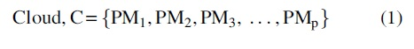
where C represents Cloud and PM represents Physical Machine hosted in cloud. For Physical machine PM1, we have:

where VM is the virtual machine.

Consider that each VM has its CPU and memory. Let the number of tasks be “k”, and each task has a different CPU user cost, memory user cost, deadline, and budget cost.

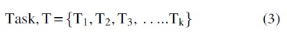
where T represents a task in the queue of the task scheduler for execution.

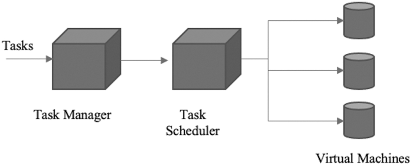
In a cloud computing environment, the task manager receives the incoming task requests and provides them to the task scheduler as shown in Figure 1. Each incoming task carries information like memory requirement, budget, cost, and deadline of the task. Based on this information, the task scheduler prioritizes the task and schedules it accordingly. The scheduler then assigns the tasks to VMs for execution. This article has proposed an ASFLA task scheduling technique for scheduling the incoming tasks by the task scheduler. The efficiency of the task scheduler depends on the speed and accuracy at which the task scheduler schedules and allocates the incoming tasks to the available VMs. The proposed ASFLA techniques provide a more efficient technique to provide faster solution as per the results obtained in Experiment and Result section.

Figure 2 provides the allocation of incoming tasks by the task scheduler based on the following parameters:

FIG. 2.

Block diagram of task scheduler scheduling tasks to VMs in the cloud computing environment. VMs, virtual machines.

CT_k is the CPU cost for task T_k. Unit of measurement is in dollar.

MT_k is the memory cost for task T_k. Unit of measurement is in dollar.

DT_k is the deadline for task T_k. Unit of measurement is in milliseconds.

BT_k is the budget cost of task T_k. Unit of measurement is in dollar.

Figure 3 provides a block diagram of an ASFLA-based scheduler for scheduling tasks to VMs in the cloud environment. With the help of the multi-objective model, we will calculate the budget cost and fitness of the task. The cost function of the incoming task and memory of the VM is added to calculate the budget cost. Allocation of the incoming tasks to available VM is performed based on the fitness as calculated by the multi-objective model.

FIG. 3.

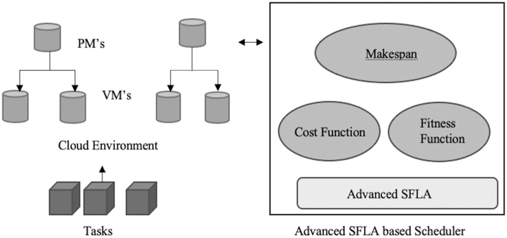
Block diagram of ASFLA-based scheduler for task scheduling in an application system hosted in the cloud environment. ASFLA, advanced shuffled frog leaping.

The proposed ASFLA algorithm divides the tasks into small memeplexes and searches for the best available solution in each memeplex. Once the best solution is achieved, it removes the worst task with the best task in the population and then shuffles the position in each memeplex, and again searches for the best solution and repeats the process until the best solution is reached.

Figure 3 provides a task scheduler based on ASFLA that allocates the tasks to VMs in a cloud environment based on the makespan, cost function, and fitness value of each incoming user task.

Task scheduling process and parameter

The main objective of the task scheduling method^5,9 is to schedule the tasks to VMs with less makespan and less budget cost. Makespan is the total time needed for executing all the tasks. Makespan of the task scheduler was calculated as the ratio of total time taken by the scheduler to process the tasks and the number of tasks that was processed. The makespan contributes to the overall efficiency of the task scheduler. Makespan determines the speed and the time taken at which the scheduler schedules the incoming tasks to the VMs. If the makespan of the task scheduler is low then the efficiency of the scheduler increases.

The cost function of CPU and memory of virtual machine Vi can be calculated by using the following equation:

CV(x) = Sum of CVcost(n) for all virtual machines

where, CVcost(n) is the CPU cost of the virtual machine

CVcost(n) can be calculated as follows: $C V_{c o s t} (n) = C_{b a s e} \times C_{n} \times T_{i j} \times C_{t r a n s}$ (4)

where,

C_base is the base cost

CV_n is the cost of the CPU of the virtual machine

T_kn is the time of processing tasks T_k in resource R_n

C_trans is transmission cost

C_base and C_trans are constants.

Calculation of cost function

The cost function is the cost of memory of the VM. To increase the efficiency of the overall application, the cost function should be as less as possible. If the cost of memory is more then, it will increase the overall budget of the application. The other way to reduce the overall budget is to utilize the memory efficiently to avoid the memory cost. The cost function can be calculated by using the below equation:

MV(x) = Summation of cost of memory for all VM MV_cost(n)

where MV_cost(n) is the cost of memory of the virtual machine

VM is the total number of virtual machines. Cost calculation for memory in VM: $M V_{c o s t (n)} (x) = M_{b a s e} (x) \times M V_{n} (x) \times t_{k n} \times M_{t r a n s} (x)$ (5)

where M_base is the base cost of memory

MV_n is the memory of the virtual machine V_n

t_kn is the time taken to process task T_k in resource

M_trans represents the cost of the memory

M_base and M_trans are constants.

Budget cost calculation

The budget cost, which is the sum of the cost function of the CPU (CV(x)) and memory of the virtual machine (MV(x)) can be stated as follows.²⁸ The budget cost is calculated in dollars: $B C (x) = C V (x) + M V (x)$ (6)

Also, Average cost = Average of budget cost.

Calculation of fitness

The fitness function can be stated as follows²⁸: $H (x) = M S (x) + B C (x)$ (7)

where MS(x) is the makespan and BC(x) is the budget cost.

Calculation of makespan

The unit of measurement is tasks executed per milliseconds. Also, $M S (x) \leq S u m m a t i o n o f D L_{i}$ (9)

where DL_i is the deadline of the task T

The deadline can be described by the following equation: $B C (x) \leq S u m m a t i o n o f B C_{k}$ (10)

where BC_k is the budget cost of task T_k

Proposed ASFLA algorithm

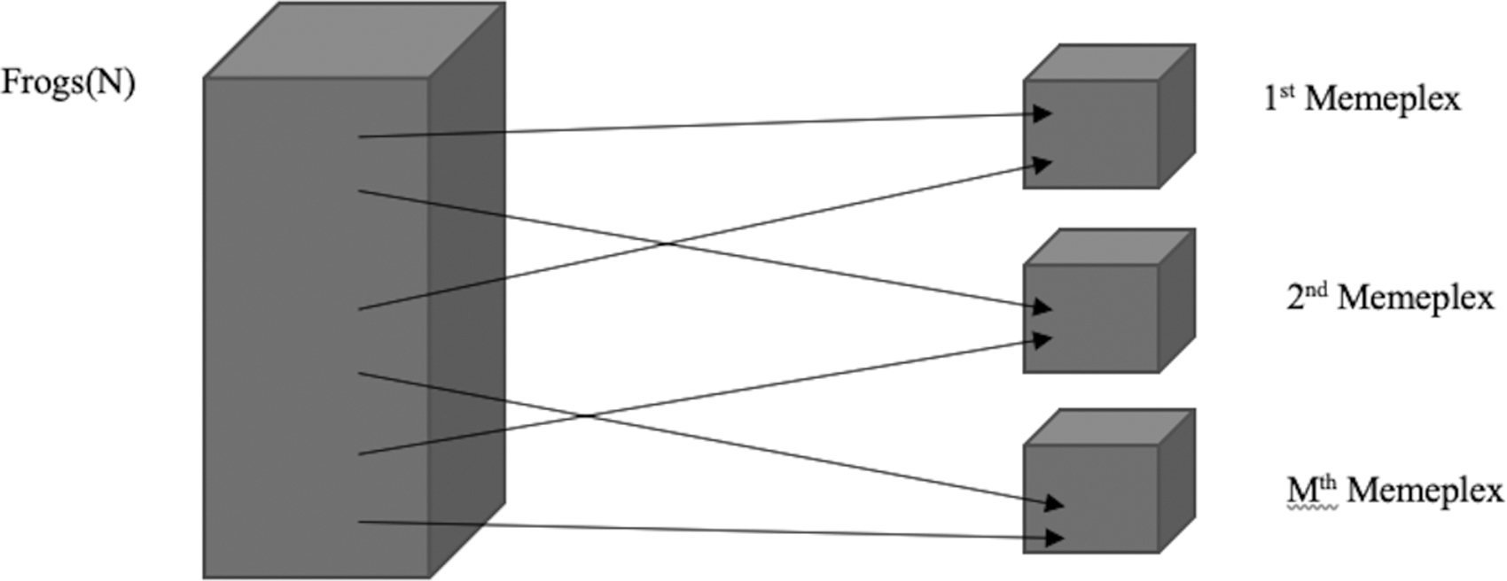
ASFLA algorithm is based on the approach that a group of frogs are searching for food. In this process, frogs interact with each other individually and exchange information about food location. In ASFLA, a set of frogs were considered as a population. This population were divided into a number of small memeplexes. Memeplex is a small portion of population where frogs are kept together and share information among those frogs kept together in the same memeplex. Memeplex can be considered as a small patch of island where few frogs from the population are kept and monitored so that they can pass information among themselves, which is considered in our study. In each memeplex, frogs of different behaviors perform a local search for food and pass the information of food source to another frog.

The frog having maximum information about the location of the food source is considered to be at the best position and the frog with minimum information about the source of food is considered to be at the worst position. In this new approach, the worst memeplex across the population was identified by calculating the average of the overall information received in each memeplex. In the next step, the position of the worst frog in that worst memeplex is identified. After one generation, the position of the frog at the best position across the population is swapped with the position of the frog at the worst position of the worst memeplex.

After this step, the position of the frog is shuffled in each memeplex and across the population. The process of shuffling of frogs to exchange information among them continues until the termination criteria are reached. The termination criteria are based on the number of generations being considered in the study. The proposed algorithm has proposed a new sorting technique to identify the worst and the best frog in the memeplex, which makes the proposed algorithm more effective compared with other frog leaping algorithms. The proposed ASFLA technique has introduced a new sorting technique of frogs in a memeplex to enhance the task scheduling using the proposed advanced frog leaping algorithm in cloud computing environment.

Steps of ASFLA Algorithm:

Step 1: Initialization

Initialize the random population(P) of frogs:

where i = 1, 2, 3, 4, …, F; j = 1, 2, 3, 4 …, D(dimension) and rand (0, 1) is a random number, which is uniformly distributed between 0 and 1.

RPop_l: Lower bound of a random population of frogs

RPop_u: Upper bound of a random population of frogs

Step 2: Sorting and distribution of frogs in memeplexes

In this step, the fitness of each frog is calculated. In the next step, memeplexes are created and each frog is distributed to memeplexes. The frogs are distributed in memeplexes using bubble sort technique in such a way that the frogs with best fitness value is placed in 1st position of each memeplex and frogs with relevant fitness value is placed in 2nd, 3rd,…n position of each memeplex.

Figure 4 provides the sorting of frogs in memeplexes.

FIG. 4.

Sorting of frogs in memeplexes.

Step 3: Local search

In this step, the frog with best, worst, and global fitness value is identified. The frog with the worst fitness function is supposed to improve through the evolutionary process in each cycle. The position of the worst frog can be updated using the following equations:

The position of frog (FP) in ith iteration can be calculated by the following equation:

where, rand (0,1) is a random integer value

X_b = Position of the frog with the best fitness value

X_w = Position of the frog with the worst fitness value

After ith iteration, the position of the frog with worst fitness can be calculated as:

Xw = current position (Xw +Di)

-Movmax ≤ Movt ≤ Movmax

where, t is the number of generations from 1 to Ngen

Movt is the frog's movement

Movmax represents maximum permissible movement

Step 4: Shuffling and Termination:

In this step, the position of the frog is shuffled to obtain the best result until the termination criteria are reached. In the proposed approach, the position of the worst frog in the memeplex is replaced with a frog with the best fitness in the population. After this step, the frogs are shuffled again and the global best and worst frog positions are determined. If the position of the frog got enhanced, then the position of the worst frog is replaced by the newly generated value, else again the best global position is determined. In this case, X_b becomes X_g.

In case of no change in the position of the worst frog, a new solution is initiated again. This iterative process continues up to the number of generation and the process is stopped once the exit criteria are reached. The exit criteria are the factor based on which the iteration process can be stopped and results can be calculated. In the proposed study, number of generations is considered as the termination criteria.

In the proposed shuffling process, the position of the best frog in the population is identified and named as X_global. The position of worst (X_worst) and best (X_best) frog in each memeplex is identified. The average of makespan in each memeplex is calculated. The memeplex with the best and worst average value of makespan is identified. The position of the worst frog of memeplex having the worst makespan is replaced with X_global and all the frogs across all memeplexes got shuffled to generate a new frog position. This shuffling process is repeated until the termination criteria are reached.

In the proposed study, the ASFLA algorithm is used by the scheduler to schedule the task to machines in a multi-objective model.

Algorithm—Advanced Shuffled Frog Algorithm

Step 1: Population initialization

Step 2: Distribution of frogs in memeplexes

Step 3: Initiate evolutionary process

Step 4: Initialize the process by setting i = 1

Step 5: while i≤ i_max

Step 6: Identify the position of the best frog in the population and name the position as X_global

Step 7: Identify the position of worst (X_worst) and best (X_best) frog in each memeplex

Step 8: Calculate the average of makespan (calculation parameter) in each memeplex

Step 9: Calculate memeplex with the best and worst average value of makespan

Step 10: Calculate the position of the best and worst frog in each memeplex

Step 11: Replace the position of worst memeplex with frog at X_global

Step 12: Shuffle the position of frogs in memeplexes to generate a new frog position

Step 13: If f(X_new) < f(X_worst)

Step 14: Set X_worst = X_new and go to Step 16

Step 15: If X_best = X_global. Go to Step 6

Step 16: i = i + 1

Step 17: End While

Step 18: The population of the frog is shuffled

Step 19: If fixed termination criterion is achieved then exit and stop execution

Result and Discussion

This section represents the results related to the experimental setup and ASFLA-based scheduler for task scheduling to the VMs in the cloud computing environment.

As per the multi-objective function, when k number of tasks are triggered to m number of physical machines with each physical machines having n VMs, then based on CPU usage cost of VM, memory usage cost of the VM and deadline of the task, an algorithm can be used to allocate the incoming tasks to VMs in cloud computing environment. The algorithm should take the above parameters as its input and provide proper best makespan, average cost, and fitness value that allows the incoming tasks to get allocated to best VM to complete the task with less task processing time. Based on the data from open sources Jenkins, the experiments are performed with different combination of data and results are calculated and compared with experiments carried out on the same data set by using already existing task scheduling techniques. The experiment details results are discussed in following section.

Experimental setup

The experiment is performed on the personal computer with the specifications mentioned in Table 1.

Table 1.

Experimental setup

Parameter	Value
Operating system	Windows 10 (64 bit)
Processor	Intel Core i5
Processor memory	8 GB
Programming language	Core Java
Programming tool	IDE Eclipse 2020-03 (4.15)

Evaluation metrics

The performance of an ASFLA-based scheduler in a cloud computing environment is determined by calculating makespan, average cost, and fitness function. In this experimental setup, the above parameters are calculated using Core java and the results are compared with already existing scheduling techniques. To obtain a comparative result, the same dataset was used to perform other scheduling studies.^28,34,35 The data sets were taken from opensource Jenkins.

Experiment and result

In the below section, three experiments were performed on different data sets. Makespan, average cost, and fitness function were calculated and are given in the following section.

Experiment I

Data set for experiment I in Table 2.

Table 2.

Data set for experiment I

Number of primary machines	40
Number of tasks	100, 200, 300, 400
Memeplex (P)	10, 15, 20
Iterations	25
CPU usage cost	0.0025 dollar per MB
Memory usage cost	0.0135 dollar per MB
Deadline	6000 milliseconds per task

CPU, central processing unit.

Sorting based on task deadline and calculation of average makespan

When the number of the tasks is 100, all the tasks are assigned to 10 memeplexes sequentially. Task T1 is assigned to the first memeplex, T2 is assigned to the second memeplex, similarly task T10 is assigned to 10th memeplex. All the tasks are assigned to memeplexes in such a way that each memeplex will have 10 tasks. For example, memeplex 1 will have task T1, T11, T21,… T91 and memeplex 2 will have task T2, T12, T22,.. T92 and so on as given in Figure 5.

FIG. 5.

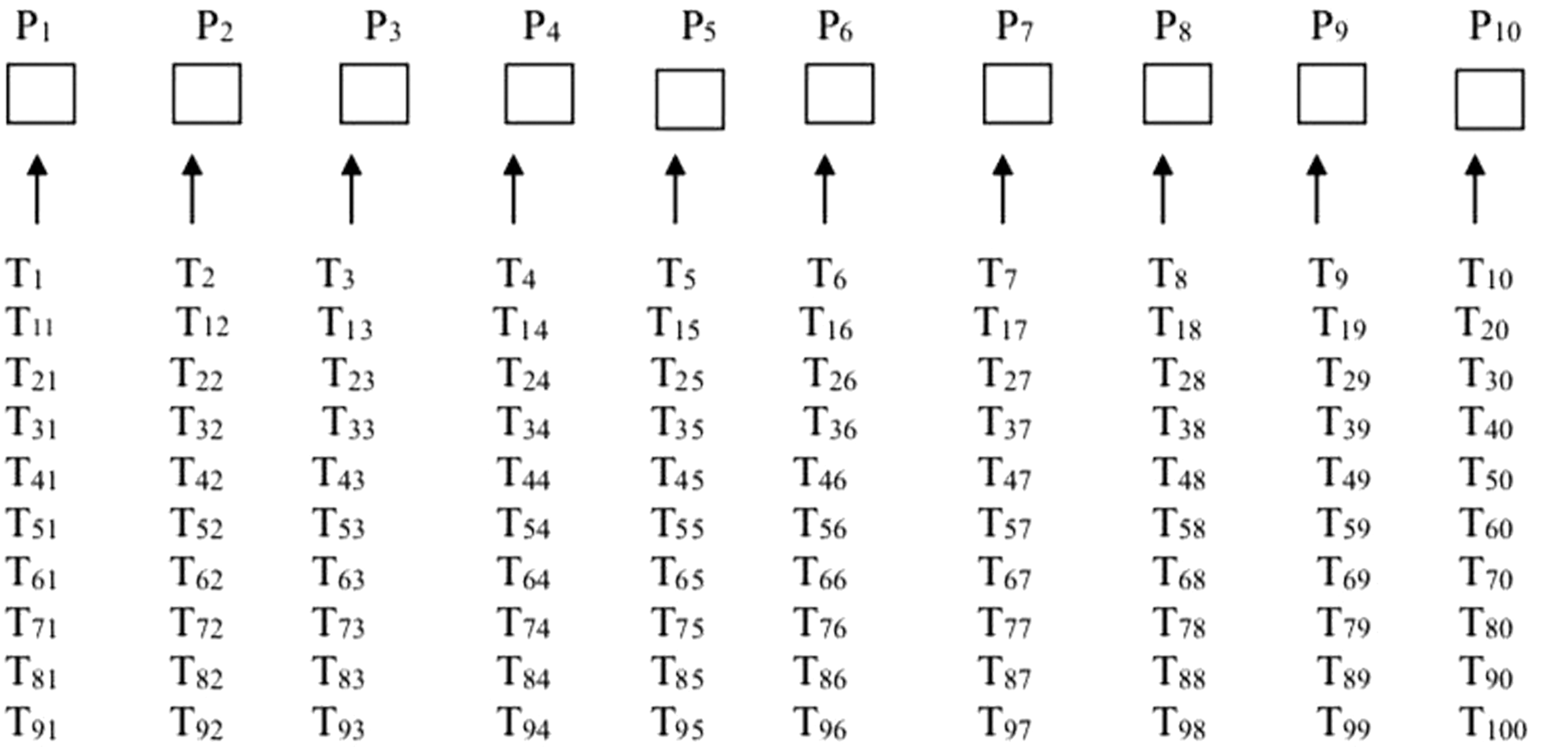
Sorting of tasks in memeplexes.

In a cloud computing environment, each task and task scheduler have its basic parameters like cost function, memory cost, memory requirement, task deadline, and budget cost. In each memeplex, the task with the lowest task deadline time is considered as worst and its position is updated as X_worst, and the task with the highest deadline time is considered as best and its position is updated as X_best. The task with the lowest deadline time in population is identified and is named X_global.

In the next step, the average makespan of all the memeplex is calculated using Eq. (4) and the memeplex with the best average makespan is identified. X_best of memeplex with the highest deadline time is replaced with X_global. After this step, the position of each task is shifted sequentially in the population and each task is shifted to the new position and a new set of tasks are generated in each memeplex. Again, the makespan of each memeplex is calculated and all the above steps are repeated 25 times. After 25 iterations, the makespan of each memeplex and the average of all memeplexes is calculated to calculate the final makespan and assign all the tasks to 40 primary machines from memeplexes.

Similarly, 200, 300, and 400 tasks are sorted into 15 and 20 memeplexes, respectively, and are assigned to 40 primary machines using the proposed ASFLA (Table 2).

Figure 6 provides the result of the makespan of the scheduler based on the proposed ASFLA algorithm in a cloud computing environment. In this experimental setup, for 100 tasks, the makespan is calculated as 7, 6, and 7 for memeplex sizes 10, 15, and 20, respectively. Similarly, when the number of tasks is increased to 200, the makespan is calculated as 6, 6, and 6 for memeplex sizes 10, 15, and 20, respectively. When the number of tasks is increased to 300 and the number of iterations is 25, then the makespan is calculated as 8, 7, and 6 for memeplex sizes 10, 15, and 20, respectively. When the number of tasks is further increased to 400, then makespan is calculated as 6, 7, and 6 for memeplex sizes (P) 10, 15, and 20, respectively.

FIG. 6.

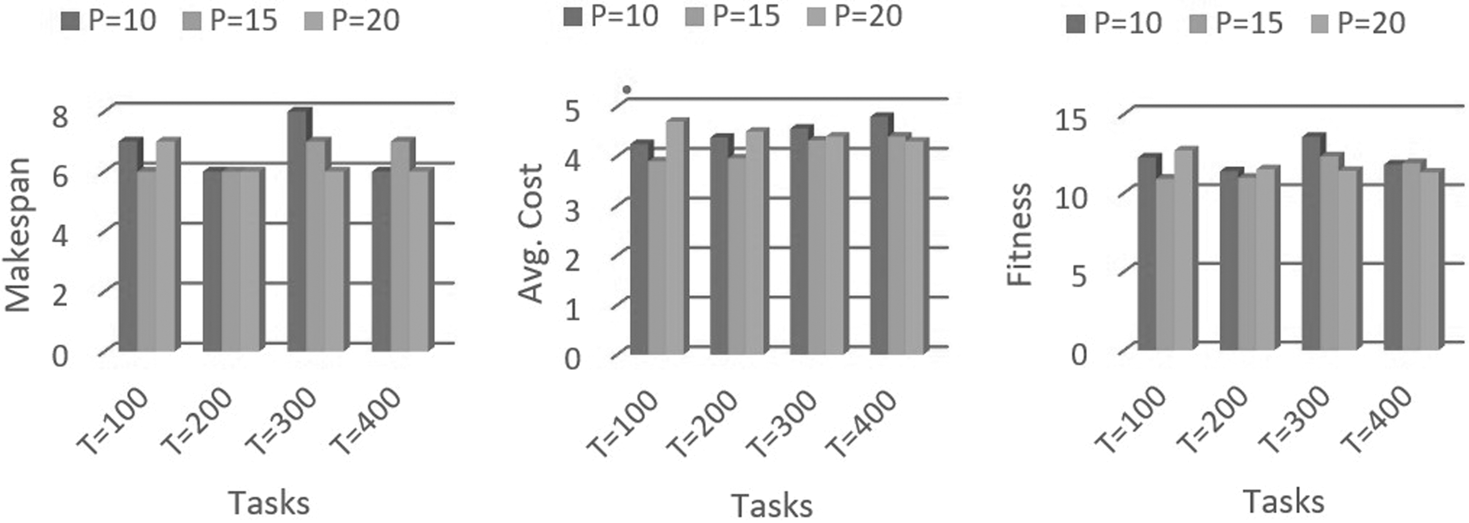
Makespan versus tasks, average cost versus tasks and fitness versus tasks graph for 25 iterations when PM = 40. PM, physical machine.

Sorting based on execution cost of task and calculation of average execution cost

In this section, the average execution cost for all incoming tasks is calculated and tasks are scheduled to primary machines using the proposed ASFLA. When the number of tasks is 100, all the tasks are assigned to 10 memeplexes sequentially. After assigning the tasks to memeplexes, the task with the highest execution cost is considered as the worst and its position is updated as X_worst, and the task with the lowest execution cost is considered as best and its position is updated as X_best. Now, the task with the lowest execution cost in population is identified and is named X_global.

In the next step, the average execution cost of all the memeplex is calculated and memeplex with low average execution cost is identified. The average execution cost is calculated by summarizing the execution cost of total tasks divided by total number of tasks in each memeplex. Now, X_best of memeplex with the lowest average execution cost is replaced with X_global. After this step, the position of each task is shifted sequentially in the population and we get a new position of each task and a new set of tasks in each memeplex. Again, the average execution cost of each memeplex is calculated and all the above steps are repeated 25 times. After 25 iterations, the average execution cost of each memeplex is calculated. In addition, the average of all memeplexes is calculated to get the final average execution cost. After this step, all the tasks from each memeplex are assigned to 40 primary machines.

Similarly, 200, 300, and 400 tasks are assigned to 15 and 20 memeplexes, respectively, and are executed by 40 primary machines using the proposed ASFLA.

As per the experimental result, when the number of incoming tasks is 100, for 25 iterations and 40 primary machines, the average cost for memeplex sizes 10, 15, and 20 is calculated as 4.38, 4.1, and 4.68, respectively. For 200 incoming tasks, the average cost is calculated as 4.27, 3.8, and 4.59, respectively, for memeplex sizes 10, 15, and 20. When the number of tasks is 300, the average cost is calculated for T = 20 becomes 4, which is less compared with T = 10 and T = 15, which is 4.233 and 4.01, respectively. When the number of tasks is further increased to 400, the average cost for memeplex sizes (P) 10, 15, and 20 is calculated as 4.76, 4.435, and 4.26, respectively.

Sorting based on fitness function and calculation of average fitness

In this section, each task is assigned to memeplexes based on their fitness function. The fitness function is calculated from Eq. (3). When the number of tasks is 100, all the tasks are assigned to 10 memeplexes sequentially. Task T1 is assigned to the first memeplex, T2 is assigned to the second memeplex, similarly task T10 is assigned to the 10th memeplex. All the tasks are assigned to memeplexes in such a way that each memeplex will have 10 tasks.

After assigning the tasks to memeplexes, the task with the highest fitness value is considered as worst and its position is updated as X_worst, and the task with the lowest fitness value is considered as best and its position is updated as X_best. Now, the task with the lowest fitness value in the population is identified and is named X_global.

In the next step, the average fitness value of tasks in each memeplex is calculated and the memeplex with the highest average fitness value is identified. Now, X_best of memeplex with the lowest average fitness value is replaced with X_global. After this step, the position of each task is shifted sequentially in population and we get a new position of each task and a new set of tasks in each memeplex. Again, the average fitness value of each memeplex is calculated and all the above steps are repeated up to 25 iterations. After 25 iterations, the average fitness value of each memeplex is calculated. In addition, the average fitness value of all memeplexes is calculated to get the overall average fitness value. After this step, the tasks from each memeplex are assigned to 40 primary machines.

Similarly, 200, 300, and 400 tasks are moved to 15 and 20 memeplexes, respectively, and are assigned to 40 primary machines using the proposed ASFLA.

Figure 6 provides the experimental results of fitness of incoming tasks based on the proposed ASFLA algorithm. In this experimental setup, for 100 tasks, the fitness is calculated as 12.25, 10.9, and 12.7 for memeplex sizes 10, 15, and 20, respectively. Similarly, when the number of tasks is 200, the fitness is calculated as 11.38, 10.96, and 11.5 for memeplex sizes 10, 15, and 20, respectively. When the number of tasks is increased to 300, the fitness is calculated as 13.56, 12.32, and 11.4, respectively, for memeplex sizes 10, 15, and 20. When the number of tasks is 400, the fitness is calculated as 11.8, 11.89, and 11.3, respectively, for memeplex sizes (P) 10, 15, and 20.

Experiment II

Dataset for experiment II in Table 3.

Table 3.

Data set for experiment II

Number of primary machines	20
Number of tasks	100, 200, 300, 400
Memeplex (P)	10, 15, 20
Iterations	50
CPU usage cost	0.0035 dollar per MB
Memory usage cost	0.0145 dollar per MB
Deadline	5000 milliseconds per task

Sorting based on task deadline and calculation of average makespan

As mentioned in Table 3, when the number of tasks is 100, all the tasks are assigned to 10 memeplexes sequentially. Task T1 is assigned to the first memeplex, T2 is assigned to the second memeplex, similarly task T10 is assigned to the 10th memeplex. All the tasks are assigned to memeplexes in such a way that each memeplex will have 10 tasks as given in Figure 5.

In each memeplex, the task with the lowest task deadline time is considered as worst and its position is updated as X_worst, and the task with the highest deadline time is considered as best and its position is updated as X_best. The task with the lowest deadline time in population is identified and is named X_global.

In the next step, the average makespan of all the memeplex is calculated using Eq. (8) and the memeplex with the best average makespan is identified. Now, X_best of memeplex with the highest deadline time is replaced with X_global. After this step, the position of each task is shifted sequentially in population and each task is shifted to a new position and a new set of tasks are generated in each memeplex. Again, the makespan of each memeplex is calculated and all the above steps are repeated to 50 iterations. After 50 iterations, calculate the makespan of each memeplex and take an average of all memeplexes to calculate the final makespan and assign all the tasks to 20 primary machines from each memeplex.

Figure 7 provides results of makespan of scheduler based on proposed ASFLA algorithm in a cloud computing environment. In this experimental setup, for 100 incoming tasks, the makespan is calculated as 6, 7, and 6 for memeplex sizes 10, 15, and 20, respectively. Furthermore, when the task is subjected to 200, the makespan is calculated as 7, 7, and 6 for memeplex sizes 10, 15, and 20, respectively. For 300 incoming tasks, the makespan is calculated as 6, 6, and 6 for memeplex sizes 10, 15, and 20, respectively. And when we have a task increased to 400, the makespan is calculated as 6, 8, and 7 for memeplex sizes (P) 10, 15, and 15, respectively.

FIG. 7.

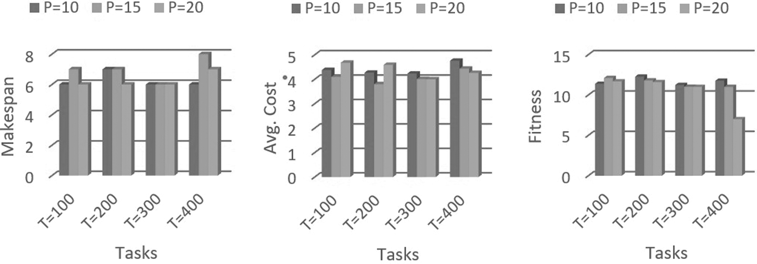
Makespan versus tasks, average cost versus tasks and fitness versus tasks graph for 50 iterations when PM = 20.

Sorting based on execution cost of task and calculation of average execution cost

In this section, the average execution cost for all incoming tasks is calculated and tasks are scheduled to primary machines using ASFLA. After assigning the tasks to memeplexes, the task with the highest execution cost and lowest execution cost is identified as X_worst, and X_best, and task with the lowest execution cost in population is identified and is named X_global.

In the next step, the average execution cost of all the memeplex is calculated and memeplex with lowest average execution cost is identified. Now, X_best of memeplex is replaced with X_global. After this step, the position of each task is shifted sequentially in population and we get a new position of each task and a new set of tasks in each memeplex. Again, the average execution cost of each memeplex is calculated and all the above steps are repeated upto 50 iterations. After 50 iterations, the average execution cost of each memeplex is calculated. In addition, the average of all memeplexes is calculated to get the final average execution cost. After this step, all the tasks from each memeplex are assigned to 20 primary machines. Similarly, 200, 300, and 400 tasks are assigned to 15 and 20 memeplexes, respectively, and are executed by 20 primary machines using the proposed ASFLA.

Figure 7 provides the results of the average cost calculated based on the proposed ASFLA algorithm in a cloud computing environment. In this experimental setup, when the number of tasks is 100, the average cost is calculated as 4.25, 3.9, and 4.7 for memeplex sizes 10, 15, and 20, respectively. Similarly, for 200 tasks, the average cost is calculated as 4.38, 3.9, and 4.5 for memeplex sizes 10, 15, and 20, respectively. When the number of tasks is 300, the average cost is calculated as 4.56, 3.96, and 4.4 for memeplex sizes 10, 15, and 20, respectively. When the number of tasks is further increased to 400, then the average cost is calculated as 4.89, 4.80, and 4.3 for memeplex sizes (P) 10, 15, and 15, respectively.

Sorting based on fitness function and calculation of average fitness

In this section, each incoming task is assigned to memeplexes based on their fitness function. The fitness function is calculated from Eq. (3). After assigning the tasks to memeplexes, the task with the highest fitness value is considered as worst and its position is updated as X_worst, and the task with the lowest fitness value is considered as best and its position is updated as X_best. Now, the task with the lowest fitness value in the population is identified and is named X_global.

In the next step, the average fitness value of tasks in each memeplex is calculated and the memeplex with the highest average fitness value is identified. Now, X_best of memeplex with the lowest average fitness value is replaced with X_global. After this step, the position of each task is shifted sequentially in population and we get a new position of each task and a new set of tasks in each memeplex. Again, the average fitness value of each memeplex is calculated and all the above steps are repeated 25 times. After 25 iterations, the average fitness value of each memeplex is calculated. In addition, the average fitness value of all memeplexes is calculated to get the overall average fitness value. After this step, the tasks from each memeplex are assigned to 40 primary machines.

Similarly, 200, 300, and 400 tasks are moved to 15 and 20 memeplexes, respectively, and are assigned to 40 primary machines using the proposed ASFLA.

Figure 7 provides results of fitness based on the proposed ASFLA algorithm in a cloud computing environment. For 100 tasks, the fitness is calculated as 11.38, 12.1, and 11.68 for memeplex sizes 10, 15, and 20, respectively. When the number of tasks is 200, fitness is calculated as 12.27, 11.8, and 11.59 for memeplex sizes 10, 15, and 20, respectively. When the number of tasks is increased to 300 and the number of iterations is 50, then fitness is calculated as 11.233, 11.01, and 11 for memeplex sizes 10, 15, and 20, respectively. When the number of tasks is further increased to 400 and the number of iterations is 50, then fitness is calculated as 11.76, 13.435, and 12.26 for memeplex sizes (P) 10, 15, and 20, respectively.

Experiment III

Dataset for experiment III in Table 4.

Table 4.

Data set for experiment III

Number of primary machines	30
Number of tasks	100, 200, 300, 400
Memeplexes (P)	10, 15, 20
Number of iterations	50
CPU usage cost	0.0045 dollar per MB
Memory usage cost	0.0155 dollar per MB
Deadline	7000 milliseconds per task

Sorting based on task deadline and calculation of average makespan

Once all the tasks are allocated to memeplexes, in each memeplex, the task with the lowest task deadline time is considered as worst and its position is updated as X_worst, and the task with the highest deadline time is considered as best and its position is updated as X_best. The task with the lowest deadline time in population is identified and is named X_global.

In the next step, the average makespan of all the memeplex is calculated using Eq. (4) and the memeplex with the best average makespan is identified. Now, X_best of memeplex with the highest deadline time is replaced with X_global. After this step, the position of each task is shifted sequentially in population and each task is shifted to the new position and a new set of tasks are generated in each memeplex. Again, the makespan of each memeplex is calculated and all the above steps are repeated to 50 iterations. After 50 iterations, calculate the makespan of each memeplex and take the average of all memeplexes to calculate the final makespan, and assign all the tasks are to 30 primary machines from each memeplex.

Figure 8 provides results of makespan of scheduler based on proposed ASFLA algorithm when the termination criteria are considered as 50 iterations. Primary machines available for task executions are considered as 30. For 100 incoming tasks, the makespan is calculated as 7, 7, and 7 for memeplex sizes 10, 15, and 20, respectively. When the total number of tasks is 200, the makespan is calculated as 7, 6, and 6 for memeplex sizes 10, 15, and 20, respectively. Next, when the number of tasks is raised to 300, the makespan is calculated as 8, 6, and 7 for memeplex sizes 10, 15, and 20, respectively. For 400 incoming tasks, the makespan is calculated as 7, 6, and 6 for memeplex sizes (P) 10, 15, and 15, respectively (Table 4).

FIG. 8.

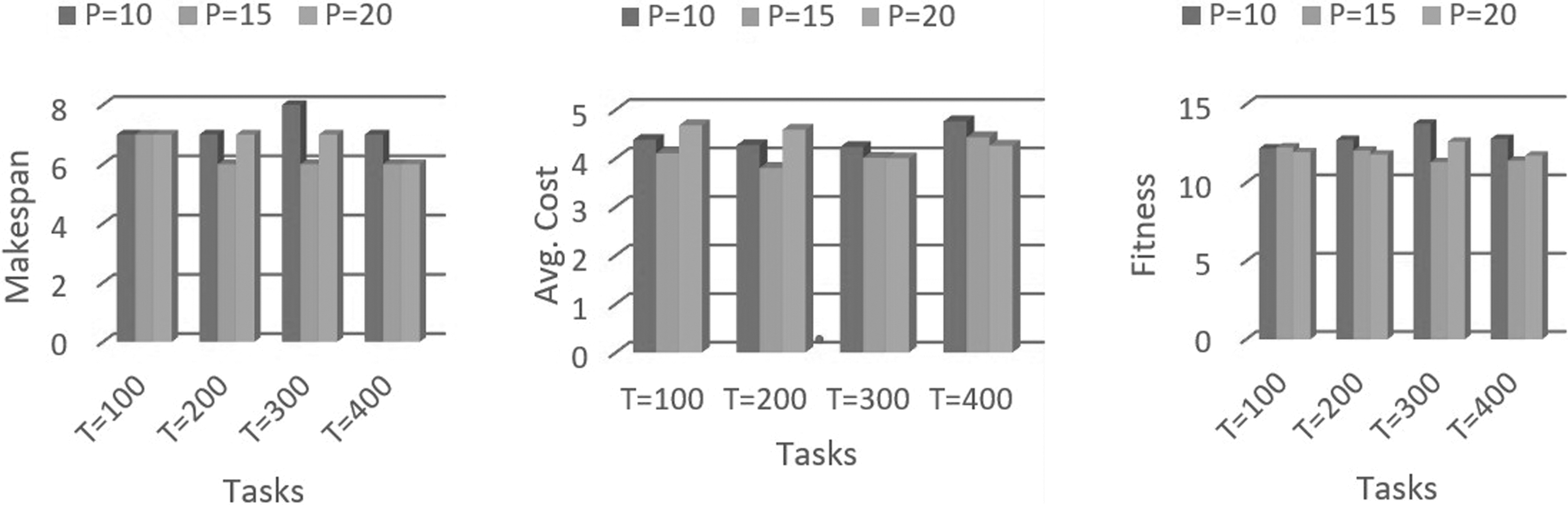
Makespan versus tasks, average cost versus tasks and fitness versus tasks graph for 50 iterations when PM = 30.

Sorting based on execution cost of task and calculation of average execution cost

In this section, the average execution cost for all incoming tasks is calculated and tasks are scheduled to primary machines using ASFLA. After assigning all the tasks to memeplexes, the task with the highest execution cost is considered as worst and its position is updated as X_worst, and the task with the lowest execution cost is considered as best and its position is updated as X_best. Now, the task with the lowest execution cost in population is identified and is named X_global.

In the next step, the average execution cost of all the memeplex is calculated and memeplex with low average execution cost is identified. Now, X_best of memeplex with the lowest average execution cost is replaced with X_global. After this step, the position of each task is shifted sequentially in population and we get a new position of each task and a new set of tasks in each memeplex. Again, the average execution cost of each memeplex is calculated and all the above steps are repeated for 50 iterations. After 50 iterations, the average execution cost of each memeplex is calculated. In addition, the average of all memeplexes is calculated to obtain the final average execution cost. After this step, all the tasks from each memeplex are assigned to 30 primary machines.

Figure 8 provides the results of the average cost calculated based on the proposed ASFLA algorithm in a cloud computing environment. In this experimental setup, when the number of tasks is 100, the average cost is calculated as 4.25, 3.9, and 4.7 for memeplex sizes 10, 15, and 20, respectively. Similarly, for 200 tasks, the average cost is calculated as 4.38, 3.9, and 4.5 for memeplex sizes 10, 15, and 20, respectively. When the number of tasks is 300, the average cost is calculated as 4.56, 3.96, and 4.4 for memeplex sizes 10, 15, and 20, respectively. When the number of tasks is further increased to 400, then the average cost is calculated as 4.89, 4.80, and 4.3 for memeplex sizes (P) 10, 15, and 15, respectively.

Sorting based on fitness function and calculation of average fitness

In the next step, the average fitness value of tasks in each memeplex is calculated and the memeplex with the highest average fitness value is identified. Now, X_best of memeplex with the lowest average fitness value is replaced with X_global. After this step, the position of each task is shifted sequentially in population and we get a new position of each task and a new set of tasks in each memeplex. Again, the average fitness value of each memeplex is calculated and all the above steps are repeated upto 50 iterations. After 50 iterations, the average fitness value of each memeplex is calculated. In addition, the average fitness value of all memeplexes is calculated to get the overall average fitness value. After this step, the tasks from each memeplex are assigned to 30 primary machines. Similarly, 200, 300, and 400 tasks are moved to 15 and 20 memeplexes, respectively, and are assigned to 30 primary machines using the proposed ASFLA.

Figure 8 provides results of fitness calculated based on the proposed ASFLA algorithm in a cloud computing environment when the termination criteria are considered as 50 iterations. Primary machines available for task executions are considered as 30.

When the number of incoming tasks is 100, then fitness is calculated as 12.18, 12.25, and 11.95 for memeplex sizes 10, 15, and 20, respectively. For 200 tasks, the fitness is calculated as 12.73, 12.05, and 11.8 for memeplex sizes 10, 15, and 20, respectively. When the number of tasks is increased to 300, fitness is calculated as 13.76, 11.31, and 12.62 for memeplex sizes 10, 15, and 20, respectively. When the number of tasks is further increased to 400, the fitness is calculated as 12.8, 11.4, and 11.725 for memeplex sizes (P) 10, 15, and 20, respectively.

Sorting based on task deadline and calculation of average makespan

Experiment IV

Table 5 provides the data to calculate the makespan of the scheduler based on the proposed ASFLA algorithm when the termination criteria are considered as 10 iterations. Primary machines available for task executions are considered as 5. For 10 incoming tasks, the makespan is calculated as 6.5, 6.66, and 7.01 for memeplex sizes 4, 5, and 6, respectively. When the total number of tasks is 20, the makespan is calculated as 6.99, 6.45, and 5.92 for memeplex sizes 4, 5, and 6, respectively. Next, when the number of tasks is raised to 30, the makespan is calculated as 7.01, 5.67, and 6.89 for memeplex sizes 4, 5, and 6, respectively. For 40 incoming tasks, the makespan is calculated as 6, 5.65, and 5.89 for memeplex sizes (P) 4, 5, and 6, respectively.

Table 5.

Data set for experiment IV

Number of primary machines	5
Number of tasks	100, 200, 300, 400
Memeplexes (P)	10, 15, 20
Number of iterations	10
CPU usage cost	0.0015 dollar per MB
Memory usage cost	0.0035 dollar per MB
Deadline	5500 milliseconds per task

Experimental result

The experiments were performed for different data sets as explained in Experiment and Result section. Experiments were also performed with low datasets. Table 6 provides the overall result with different datasets.

Table 6.

Experimental result

Parameter	Result
Makespan	6
Average cost	4
Fitness	10

Comparative result

In this section, the results obtained experimentally for Makespan and Average Cost in cloud environment using the proposed ASFLA-based task scheduler were compared with the preexisting algorithms like whale optimization-based scheduler (W-Scheduler),³⁴ inverted ant colony optimization (IACO) algorithm,³⁶ static learning particle swarm optimization (SLPSO-SA),^39,40 and sliced particle swarm optimization (SPSO-SA).^39–42 For comparative purposes, the same data set was used across all algorithms to obtain consistent results.²⁸ From Table 7, it is evident that the makespan of 6, which was obtained through the proposed algorithm, is much better compared with the rest of the makespan results that were obtained using the other scheduling methods. It is also evident that the lowest average cost of 4 was obtained through this proposed model.

Table 7.

Comparative result

	ASFLA-based scheduler	W-Scheduler ³⁴	IACO ³⁶	SLPSO-SA ⁴⁰	SPSO-SA ⁴⁰
Makespan	6	7	15	30	15
Average cost	4	5.8	16	14	13

ASFLA, advanced shuffled frog leaping; IACO, inverted ant colony optimization; SLPSO-SA, static learning particle swarm optimization; SPSO-SA, sliced particle swarm optimization; W-Scheduler, whale optimization–based scheduler.

A comparative result of makespan and average cost calculated for different scheduling algorithms is given in the graph in Figure 8. The y-axis of the graph represents the value of makespan, and average cost. The x-axis of the graph represents the different scheduling algorithms when the number of tasks is 100, 200, 300, and 400 as given in Table 7. Figure 9 provides the value of Makespan and Average cost calculated for tasks 100, 200, 300, and 400 using different scheduling algorithms. From the table, it is observed that the value of makespan and average cost reduced for the proposed algorithm as compared with other algorithms.

FIG. 9.

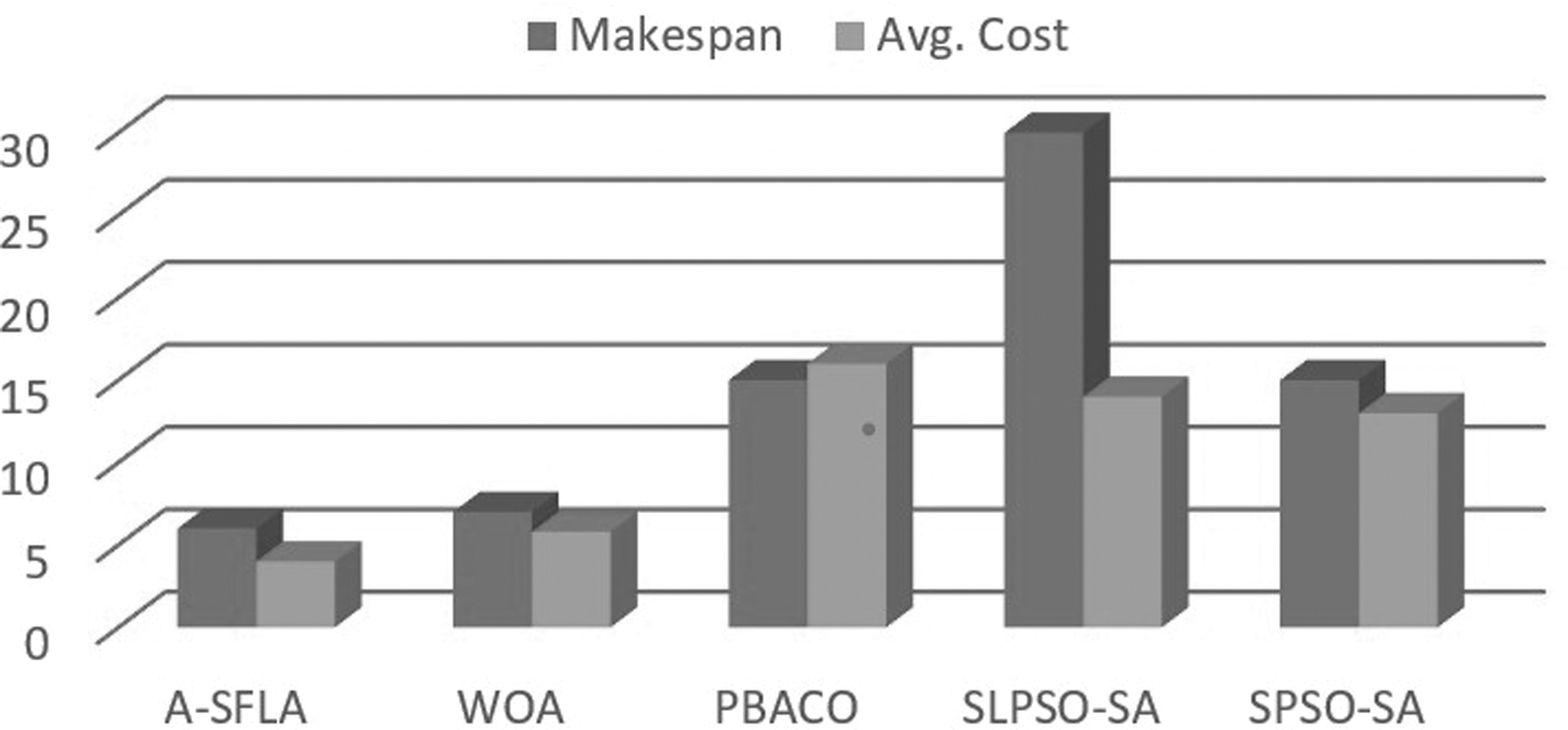
Graph showing the comparison of makespan and the average cost for different scheduling algorithms.

Conclusion

Task scheduling has become a key factor in determining the efficiency of a system. The task scheduler should be efficient enough to schedule the high volume of incoming tasks to machines based on a certain parameter that allows the task with the highest priority to be executed first as compared with the task with the least priority. The major problem in a cloud computing environment is that the task schedulers are not so efficient to effectively schedule the incoming task based on the task's priority as was demonstrated in this article. In the proposed work, the ASFLA algorithm–based task scheduler was proposed, which can effectively schedule the incoming tasks based on the parameters like makespan, average cost, and fitness for an application system based on the cloud computing environment.

The proposed method has proved to be very useful to maintain the efficiency and performance of the application system in a cloud computing environment in case of the heavy load of incoming data. The proposed model was tested experimentally and the results were obtained for heavy load and different experimental parameters like the number of primary machines, the number of iterations, and the number of memeplexes. To get a consistent comparative result, the experimental results of the proposed SFLA-based task scheduler was compared with other scheduler based on existing scheduling techniques like W-Scheduler, IACO, SLPSO-SA, and SPSO-SA. From the comparative results, it was evident that the proposed SFLA algorithm–based scheduler schedules the tasks to VMs with most minimum makespan of 6 and average cost of 4. In the future this proposed algorithm can be used by the scheduler to schedule the incoming task to VMs in the cloud computing environment. The proposed algorithm is applicable for any data set and any load condition.

Footnotes

Authors' Contributions

All authors have equally contributed in conceptualization, methodology, experiment, writing—original draft, analysis and review of the article.

Author Disclosure Statement

No competing financial interests exist.

Funding Information

No funding was received for this article.

Abbreviations Used

References

Namasudra

, Roy

, Balusamy

Cloud computing: Fundamentals and re-search issues. In: Second International Conference on Recent Trends and Challenges in Computational Models (ICRTCCM); 2017.

Sasubilli

, Venkateswarlu

. Cloud computing security challenges, threats and vulnerabilities. In: IEEE 6th International Conference on Inventive Computation Technologies (ICICT);, 2021; doi: 10.1109/ICICT50816.2021.9358709

Peng

, Huang

, Zhao

, et al. Intelligent computation offloading and resource allocation in IIoT with end-edge-cloud computing using NSGA-III. IEEE Trans Netw Sci Eng, 2022; doi 10.1109/TNSE.2022.3155490

, Li

Secure and dynamic outsourcing computation of machine learning in cloud computing. In: Cyberspace Safety and Security, 11th International Symposium, CSS 2019, Guangzhou, China, December 1–3, Proceedings, Part II; 2019; pp. 285–292.

Chen

, Luo

, Li

, et al. A training-integrity privacy-preserving federated learning scheme with trusted execution environment. Inform Scis, 2020; 522:69–79.

Blair

, Bi

, Mulvenna

. Aggregated topic models for increasing Social media topic coherence. Appl Intell, 2020; 50(1):138–156.

, Bhatia

, Kapoor

Intelligent systems and applications. In: Proceedings of the 2019 Intelligent Systems Conference, IntelliSys, 2019, London, UK, September 5–6, Volume 1 Advance in Intelligent Systems and Computing 1037, Springer; 2020, ISBN 978-3-030-29515-8.

Liu

, Hou

, Huang

, et al. Secure and efficient sharing of authenticated energy usage data with privacy preservation. Comput Secur, 2020; 92:101756.

Lin

, Zhang

, Luo

, et al. Software vulnerability discovery via learning multi-domain knowledge bases. IEEE Trans Depend Secure Comput, 2019;(99):1–1; doi: 10.1109/TDSC.2019.2954088

10.

Abualigah

, Alkhrabsheh

. Amended hybrid multi-verse optimizer with genetic algorithm for solving task scheduling problem in cloud computing. J Supercomput, 2022; 78:740–765.

11.

Mei

, Li

, Ouyang

, et al. A profit maximization scheme with guaranteed quality of service in cloud computing. IEEE Trans Comput, 2015; 64(11):3064–3078.

12.

Shen

, Yang

, Vijayakumar

, et al. A privacy-preserving and untraceable group data sharing scheme in cloud computings. IEEE Trans Depend Secure Comput, 2022:19(4):2198–2210.

13.

Razaque

, Vennapusa

, Soni

, et al. Task scheduling in Cloud computing. In: IEEE Long Island Systems, Applications, and Technology Conference (LISAT);, 2016; doi: 10.1109/LISAT37856.2016

14.

Katal

, Dahiya

, Choudhury

. Energy efficiency in cloud computing data center: A survey on hardware technologies. Cluster Comput, 2022; 25:675–705.

15.

, Dai

MCW

, Qiu

. Energy optimization with dynamic task scheduling mobile cloud computing. IEEE Syst J, 2017; 11(1):1–10.

16.

Dai

, Lou

, Lu

A task scheduling algorithm based on genetic algorithm and ant colony optimization algorithm with multi-QoS constraints in cloud computing. In: IEEE 7th International Conference on Intelligent Human-Machine Systems and Cybernetics; 2015.

17.

, Hu

, et al. Cloud task and virtual machine allocation strategy in cloud computing environment. In: International Conference on Network Computing and Information Security, NCIS 2012, Network Computing and Information Security; 2012; pp. 113–120.

18.

Gawali

, Shinde

. Task scheduling and resource allocation in Cloud computing using a heuristic approach. J Cloud Comput, 2018; 7(4); doi: 10.1186/s13677-018-0105-8

19.

Keshanchi

, Navimipour

. Priority-based task scheduling in the cloud systems using a memetic algorithm. J Circ Syst Comput, 2016; 25(10):1650119.

20.

Dahal

, Hossain

, Varghese

, et al. Scheduling in multiprocessor system using genetic algorithms. In: Computer Information Systems and Industrial Management Applications, CISIM '08. 7th; 2008.

21.

Cheng

, Li

, Wang

. An energy-saving task scheduling strategy based on vacation queuing theory in cloud computing. Tsinghua Sci Technol, 2015; 20(1):28–39.

22.

Dong-Yun

, Ping

, Luowei

, et al. A novel particle swarm optimization algorithm. In: Computer Science, IEEE International Conference on Software Engineering and Service Sciences; 2010.

23.

Abrishami

, Naghibzadeh

, Epema

Cost-driven scheduling of grid workflows using partial critical paths. In: 11th IEEE/ACM International Conference on Grid Computing; 2010.

24.

Chen

, Xie

, Li

, et al. Efficient task scheduling for budget-constrained parallel applications on heterogeneous cloud computing systems. Future Gener Comput Syst, 2017; 74:1–11.

25.

Liu

, Fan

, Buyya

A deadline-constrained multi-objective task scheduling algorithm in Mobile Cloud environments. IEEE Access, 2018:99.

26.

Lin

, Wang

, Xie

, et al. Energy and performance-aware task scheduling in a mobile cloud computing environment. In: Proc IEEE Int Conf Cloud Comput; 2014; pp. 192–199.

27.

Haidri

, Katti

, Saxena

. Cost-effective deadline aware scheduling strategy for workflow applications on virtual machines in cloud computing. J King Saud Univ Comput Inform Sci, 2020; 32(6):666–683.

28.

Zhong

, Chen

, Zhai

, et al. Virtual machine-based task scheduling algorithm in a cloud computing environment. Tsinghua Sci Technol, 2016; 21(6):660–667.

29.

Geng

, Mao

, Xiong

, et al. An improved task scheduling algorithm for scientific workflow in the cloud computing environment. Clust Comput, 2019; 22:1–10.

30.

Zhen

, Song

, Chen

. Dynamic resource allocation using virtual machines for cloud computing environment. IEEE Trans Parallel Distrib Syst, 2013; 24(6):1107–1117.

31.

Xiaolong

, Cao

, Wang

. Resource pre-allocation algorithms for low-energy task scheduling of cloud computing. J Syst Eng Electron, 2016; 27(2):457–469.

32.

Han

, Du

, Chen

, et al. Minimizing monetary costs for deadline constrained workflows in cloud environments. IEEE Access, 2020;(99):1–1.

33.

Mohammed

, Umar

, Rashid

. A systematic and meta-analysis survey of whale optimization algorithm. Comput Intell Neurosci, 2019(1):25; doi: 10.1155/2019/8718571

34.

Sreenu

, Sreelatha

W-Scheduler: Whale Optimization for Task Scheduling in Cloud Computing. Switzerland: Springer Science, Business Media, LLC; 2017.

35.

Chen

, Cheng

, Liu

, et al. A WOA-based optimization approach for task scheduling in cloud computing systems. IEEE Syst J, 2020; doi: 10.1109/JSYST.2019.2960088

36.

Azad

, Navimipour

, Zadeh

. A fuzzy-based method for task scheduling in the cloud environments using inverted ant colony optimization algorithm. Int J Bio-Inspir Comput, 2019; 14(2):125.

37.

Milan

, Rajabion

, Darwesh

, et al. Priority-based task scheduling method over cloudlet using a swarm intelligence algorithm. Clust Comput, 2019; 23(8); doi: 10.1007/s10586-019-02951-z

38.

Jacob

, Pradeep

. A multi-objective optimal task scheduling in cloud environment using cuckoo particle swarm optimization. Wireless Person Commun, 2019; 109(1):315–331.

39.

Liu

, Gao

, Zhang

, et al. Solving NP-hard problems with Physarum-based ant colony system. IEEE/ACM Trans Comput Biol Bioinform, 2017; 14(1):108–120; doi: 10.1109/TCBB.2015.2462349

40.

Xiao

, Yu

A newly self-adaptive strategy for the PSO. Proc Int Conf Natural Comput, 2008; pp. 96–400.

41.

Zuo

, Zhang

, Tan

. Self-adaptive learning PSO-based deadline constrained task scheduling for hybrid IaaSCloud. IEEE Trans Autom Sci Eng, 2014; 11(2):564–573.

42.

Liang

, Guo

, Liu

, et al. A self-adaptive dynamic particle swarm optimizer. In: IEEE Congress on Evolutionary Computation (CEC); 2015.

43.

Sharma

TK.

Performance Optimization of the Paper Mill using Opposition based Shuf fled frog-leaping algorithm. Int J Comput Inform Syst Ind Manag Appl, 2017; 9(2017):173–180.

44.

Zhang

, Zhao

, Leng

. A hyper-heuristic algorithm for time-dependent green location routing problem with time windows. IEEE Access, 2020; 8.

45.

Monisha

, Mekala

, Pradeep

, et al. A study on QoS based task scheduling using meta-heuristic algorithms in cloud environment. In: International Conference on Intelligent Computing and Control Systems (ICCS); 2019.

46.

Kheirollahpour

, Jazayeriy

, Rabiei

A heuristic-based task scheduling method for reducing waiting time in cloud environment. In: 27th Iranian Conference on Electrical Engineering (ICEE), IEEE. 2019.

47.

Brodsky

, Panferov

, Nebylov

, et al. Integrated navigation, and distributed control intelligent transport system. In: 27th Saint Petersburg International Conference on Integrated Navigation Systems (ICINS); 2020.

48.

Calabuig

, Martín-Sacristán

, Monserrat

, et al. Distribution of road hazard warning messages to distant vehicles in intelligent transport systems. IEEE Trans Intell Transport Syst, 2018;19(4).