Computational Efficient Approximations of the Concordance Probability in a Big Data Setting

Abstract

Performance measurement is an essential task once a statistical model is created. The area under the receiving operating characteristics curve (AUC) is the most popular measure for evaluating the quality of a binary classifier. In this case, the AUC is equal to the concordance probability, a frequently used measure to evaluate the discriminatory power of the model. Contrary to AUC, the concordance probability can also be extended to the situation with a continuous response variable. Due to the staggering size of data sets nowadays, determining this discriminatory measure requires a tremendous amount of costly computations and is hence immensely time consuming, certainly in case of a continuous response variable. Therefore, we propose two estimation methods that calculate the concordance probability in a fast and accurate way and that can be applied to both the discrete and continuous setting. Extensive simulation studies show the excellent performance and fast computing times of both estimators. Finally, experiments on two real-life data sets confirm the conclusions of the artificial simulations.

Introduction

Since the beginning of this century, technological advances dramatically changed the size of data sets as well as the speed with which these data have to be processed, analyzed, and evaluated. Modern data may have a huge number of observations and/or a very large number of dimensions. Recently, data are growing at an explosive rate and these massive data sets are collected at high speed from different sources, for example, results of sensors in an industrial process or in health care, spatial data from mobile devices, etc.

These data are often used to get insights into a certain process, which are typically obtained by predicting one response variable by using all the other explanatory variables. Many statistical models can be used for this prediction task that will turn data into knowledge and hence, it is of utmost importance to compare the performance of these various models. In this article, it will be shown how to efficiently compute the concordance probability, a popular measure of the predictive ability of both classification and regression problems. We will focus on the presence of a huge number of observations, to which the computing time of this measure is particularly sensitive.

For evaluating the quality of a binary classifier, the focus typically lies on the discriminatory ability of the model. For more information on the different aspects of the predictive ability, such as the difference between the discriminatory ability and the calibration, we refer to Steyerberg et al.¹ The most widely used performance measure to check the discriminatory ability of a binary classifier is the area under the receiver operating characteristic (ROC) curve (AUC); see, for example, the work of Liu et al., Razavian et al., and De Cnudde et al.^2–4 Note that the construction of the ROC curve was suggested in the electronic signal detection theory.⁵

It is known that the AUC in case of a binary response variable equals exactly the concordance probability, also called the C-index.⁶ The concordance probability corresponds to the probability that a randomly selected subject with outcome $Y = 1$ has a higher predicted probability $π (X) = P (Y = 1 | X)$ than a randomly selected subject with outcome $Y = 0$ , where X corresponds to the vector of variables⁷: $C = P (π (X_{i}) > π (X_{j}) | Y_{i} = 1, Y_{j} = 0) .$ (1)

A pair of observations with their predictions that satisfies the above condition is called a concordant pair. Hence, the concordance probability can also be defined as the probability that a randomly selected comparable pair of observations with their predictions is a concordant pair. The concordance probability, defined in Equation (1), normally ranges between 0.5 and 1, and the closer it is to 1, the better its discriminatory ability.

If its value drops below 0.5, the predictions are consistently inconsistent. For a sample of size n, the concordance probability typically is estimated as the ratio of the number of concordant pairs n_c over the number of comparable pairs n_t: $\begin{matrix} Ĉ & = \frac{n_{c}}{n_{t}} = \frac{{\hat{π}}_{c}}{{\hat{π}}_{c} + {\hat{π}}_{d}} \\ = \frac{\sum_{i = 1}^{n - 1} \sum_{j = i + 1}^{n} I (\hat{π} (x_{i}) > \hat{π} (x_{j}), y_{i} = 1, y_{j} = 0)}{\sum_{i = 1}^{n - 1} \sum_{j = i + 1}^{n} I (\hat{π} (x_{i}) \neq \hat{π} (x_{j}), y_{i} = 1, y_{j} = 0)}, \end{matrix}$ (2)

where the value ${\hat{π}}_{c}$ (respectively ${\hat{π}}_{d}$ ) refers to the estimated probability that a comparable pair is concordant (respectively discordant) and $I (\cdot)$ to the indicator function.

For observation i, y_i and $\hat{π} (x_{i})$ correspond to the observed outcome and estimated predicted probability with X _i the vector of observed variables respectively. Note that the extra condition $\hat{π} (x_{i}) \neq \hat{π} (x_{j})$ is added to the denominator to ensure that no ties in the predictions are taken into account.⁸ Ties namely attenuate the concordance probability to 0.5, depending on the distribution of the observations over the different risk groups, which is undesirable.⁹

According to Yan and Greene,⁸ it depends on the context whether one wants to ignore ties. An estimator should, therefore, be able to handle both situations. Since ties only influence the actual definition of the comparable and concordant pairs, the choice of whether to include ties does not influence the expression of any definition or estimator presented here.

See Yan and Greene⁸ for a more detailed treatment of the subject of ties on the concordance probability. However, the approximations that we will discuss in this article are still applicable when one wants to include ties in the predictions, something that is often done in the classical AUC estimator.

As can be seen in Equation (2), calculating this C-index can be very time consuming for large data sets. Therefore, research was conducted to find approximations that reduce the time complexity for calculating such a discriminatory measure in a discrete setting. For example, Bouckaert¹⁰ provides a method for incrementally updating exact AUC curves and for calculating approximate AUC curves.

A number of researchers have attempted to approximate the AUC by smooth functions,^11–13 or more specifically polynomials.¹⁴ The most popular algorithm is introduced by Fawcett,¹⁵ where the ROC curve is determined efficiently such that the AUC can be calculated as the area under the ROC curve. This area is obtained by approximating the integral by the trapezium rule.

In this article, two additional approximations will be presented, which do not rely on the link between the concordance probability and the area under the ROC curve.

k-means approximation: rather than working with the predictions of all observations of the data set, the predictions of the observations of each outcome class are reduced to the predictions of the centroids of k clusters. Afterward, Equation (2) is applied to predictions of the latter centroids only. Due to its favorable scaling to large data sets, the k-means clustering algorithm will be used.

Marginal approximation: For each observation of a given outcome class, its prediction is compared with all predictions of the other outcome class, meaning that there is no correlation between the pairs of both outcome classes that are considered during the estimation process. Hence, by approximating the distribution of predictions of both outcome classes separately by discrete bins and by computing the concordance probability using these bins rather than each separate observation in Equation (2), the concordance probability can be computed more efficiently.

When the response variable Y is continuous, the discriminatory ability of the model can also be of interest, especially when the ranking of the observations is of higher importance than obtaining well-calibrated predictions. Typical examples are the modeling of the claim size distribution of a non-life insurance product, or the modeling of a lifetime distribution in a churn analysis. Note that the concordance probability is particularly popular within the field of survival analysis, and many estimation methods have been proposed to compute the concordance probability in the presence of right censoring.^16,17 As such, the basic Definition (1) is typically adapted as: $C = P (π (X_{i}) > π (X_{j}) | Y_{i} > Y_{j}),$ (3)

where $π (X_{i})$ represents the predicted value of Y_i. However, in some situations, distinguishing nearly identical observations has little practical importance. Consequently, the basic definition in Equation (3) can be extended as follows: $C (ν) = P (π (X_{i}) > π (X_{j}) | Y_{i} - Y_{j} > ν),$ (4)

where $ν \geq 0$ . In other words, the difference between the considered observations is at least $ν$ . Note that in this continuous setting, there is no link with the area under the ROC curve.

As a result, the aforementioned research is not suitable for this setting in case of a large data set. To our knowledge, the present article is the first one that focuses on approximating the concordance probability in a fast and efficient manner in the continuous setting. The aforementioned k-means and marginal approximation will be adapted to the continuous setting.

Summarized, we present in this article two computationally efficient approximations of the concordance probability for big data, in both a discrete and continuous setting, the k-means and marginal approximation. The remainder of this article is structured as follows. The k-Means and Marginal Approximation section presents a detailed explanation of the two proposed approximations. The good performance of both estimators of the concordance probability is verified in an extensive simulation study in the Simulations section. Finally, we illustrate the practical applications of this work on two real-life examples in the Real-Life Examples section. The main findings and suggestions for further research are summarized in the Conclusion section.

k-Means and Marginal Approximation

In this section, two approximations of the concordance probability are presented. One approximation makes use of the k-means clustering algorithm and will therefore be called the k-means approximation. The other one takes advantage of the structure of the estimation process of the concordance probability and will be denoted the marginal approximation. The first subsection focuses on the discrete setting, meaning that the response variable is binary. The second subsection considers the continuous setting, where the response variable is continuous.

Discrete setting

In this subsection, we consider the situation of a binary response variable Y. The k-means approximation can be obtained by separately applying a clustering algorithm to the predictions of each group in the definition of the concordance probability. The number of clusters k will then determine the level of approximation, hence a more precise estimate will be obtained as k increases. When the clustering algorithm is applied, only the cluster centroids will be considered for estimating the concordance probability.

In other words, all cluster centroids of each group will be compared with one another. The importance of each cluster by cluster comparison is weighted by the probability that a randomly selected pair of observations belongs to the respective clusters, or:

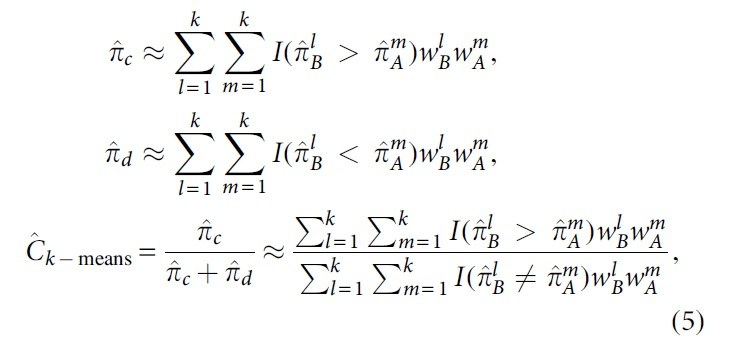
where subscript B (respectively A) refers to the group of observations of which the predictions are supposed to be higher (respectively lower) than the ones of subscript A (respectively B). The denominator of the estimator is needed to eliminate the effect of ties on the predictions. Moreover, ${\hat{π}}_{*}^{l}$ is the centroid of the l-th cluster of group * and $w_{*}^{l}$ the weight of the l-th cluster of group *. The latter is estimated by computing the percentage of observations of group * that belongs to cluster l, such that by definition $\sum_{l = 1}^{k} w_{*}^{l} = 1$ .

The marginal approximation is obtained by taking advantage of a structure that can be found in the estimation process of the concordance probability. For each observation of a given group, its prediction is compared with all predictions of the other group. As such, no correlation is present between the pairs $(π_{A}, π_{B})$ , yielding the following expression for the bivariate distribution $F_{π_{A}, π_{B}} (π_{A}, π_{B})$ : $F_{π_{A}, π_{B}} (π_{A}, π_{B}) = F_{π_{A}} (π_{A}) F_{π_{B}} (π_{B}),$

where $F_{π_{A}} (π_{A})$ and $F_{π_{B}} (π_{B})$ correspond to the marginal distributions of $π_{A}$ and $π_{B}$ , respectively.

Hence, when a grid with the same q boundary values $τ = (τ_{0} \equiv - \infty, τ_{1}, \dots, τ_{q}, τ_{q + 1} \equiv + \infty)$ for the marginal distribution of both groups is placed on top of the latter bivariate distribution, the probability that a pair belongs to any of the delineated regions only depends on the marginal distributions $F_{π_{A}} (π_{A})$ and $F_{π_{B}} (π_{B})$ . In Figure 1, an example is shown where every pair of predictions of a given data set is plotted out. A grid is added to the scatterplot, which delineates the different regions that are used to compute the marginal approximation.

FIG. 1.

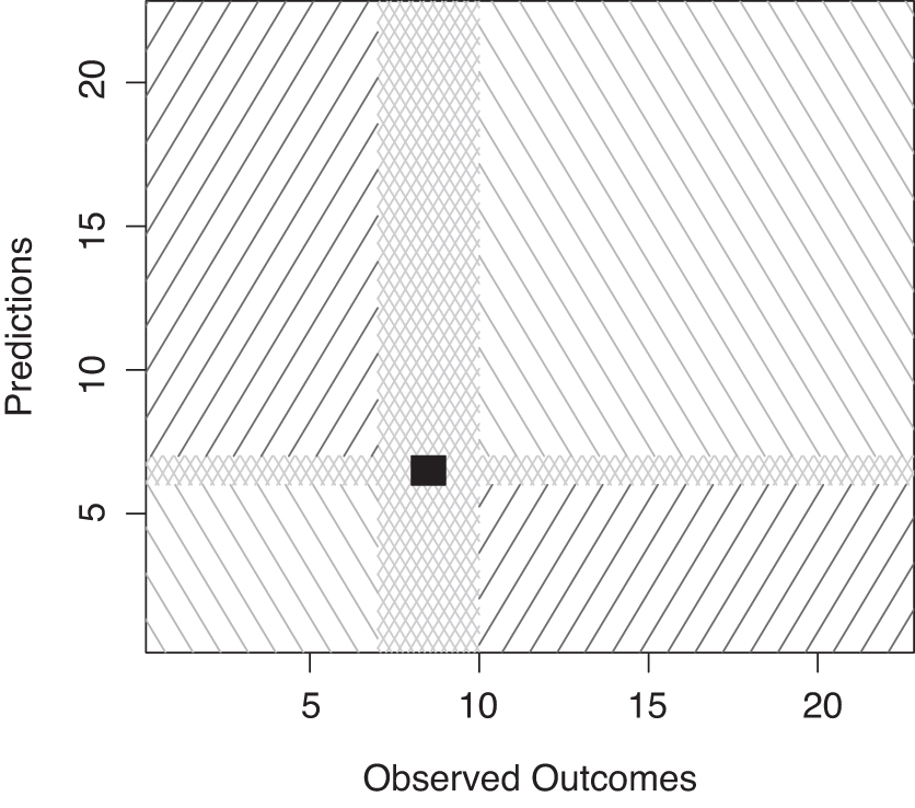
Scatter plot showing the different pairs that are considered in the estimation of the concordance probability. In dashed blue lines the grid lines are shown, hereby delineating the different regions of the grid.

In the next step, three different regions in the two dimensional space can be determined: regions that only contain concordant pairs, regions that contain only discordant pairs, and regions that also contain ties (induced by the grid structure). As such, the latter region is considered to be a region of incomparable pairs only. For the ease of presentation, we assume that the q boundaries are the same for both groups, but this is not an absolute necessity.

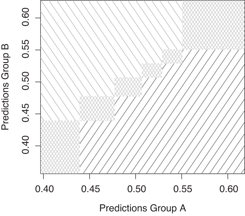
Remember that it is assumed that all observations of group A have a lower observed outcome value than all the observations of group B, and that the values of group A (respectively B) are plotted on the X (respectively Y)-axis. Therefore, all concordant pairs are located in the upper left part of the support of $F_{π_{A}, π_{B}} (π_{A}, π_{B})$ , whereas all discordant pairs are in the lower right part of the support of $F_{π_{A}, π_{B}} (π_{A}, π_{B})$ , and the incomparable pairs are in between both. In Figure 2, the downward dashed region (in green) corresponds to the region of the concordant pairs, the upward dashed region (in red) to the region of the discordant pairs, and the upward and downward dashed region (in gray) to the region of the incomparable pairs. This coloring scheme serves as an interpretation of the grid that was overlaid in Figure 1 concerning the interpretation of the different delineated regions regarding the marginal approximation.

FIG. 2.

The different regions of the grid, shown in Figure 1, in which the concordant pairs (downward dashed region, in green), the discordant pairs (upward dashed region, in red), and incomparable pairs (upward and downward dashed region, in gray) are highlighted.

Since only both marginal distributions $F_{π_{A}} (π_{A})$ and $F_{π_{B}} (π_{B})$ are needed to compute the probability that a pair belongs to a region of the support of $F_{π_{A}, π_{B}} (π_{A}, π_{B})$ , the concordance probability can be estimated as follows:

Note that this methodology only yields an approximation of the estimated concordance probability of Equation (2), and that the accuracy improves as q increases. Although $τ$ can be determined in many ways, we strongly recommend to base it on a set of evenly spaced percentiles of the empirical distribution of the predictions of both group A and B jointly. This is motivated by the easiness of determining the number of observation-prediction couples in each grid.

Continuous setting

Here, we consider the situation of a continuous response variable Y. Since the data structure and the design of the concordance probability is entirely different for the continuous setting as compared with the discrete setting, the approximations that were proposed in the Discrete Setting section (subsection of k-Means and Marginal Approximation section) will not necessarily work for this new setting. One of the key points underpinning these approximations is the existence of two independent groups. In case of a continuous response variable, two of such groups cannot be defined and therefore the previous approximations need to be adapted to the continuous setting.

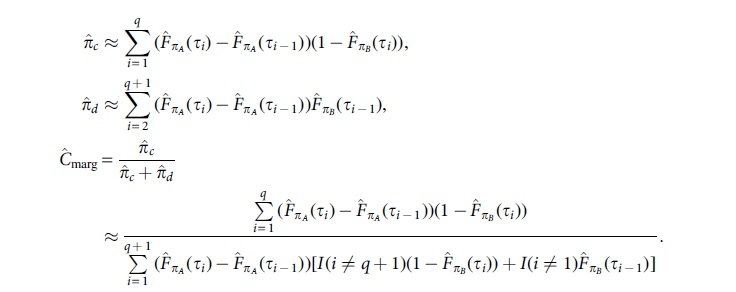
Based on Equation (4), the large data set can only be reduced to a smaller set of clusters, when these clusters of observations are jointly constructed based on their observed outcomes and predictions. All these clusters are uniquely characterized by their observed outcome, prediction and weight, the latter being determined by the number of observations that pertain to the cluster at hand. As a result, Equation (4) can be computed while using only these representations of the clusters,

where y^l and ${\hat{π}}^{l}$ are the observed outcome and the prediction of the representation of the l-th cluster respectively; which is the centroid in case of k-means.

w^l is the weight of the l-th cluster that is estimated by computing the percentage of observations belonging to cluster l, such that by definition $\sum_{l = 1}^{k} w^{l} = 1$ . Note that the number of clusters, necessary to obtain a good approximation, is likely much higher for this definition than for Definition (5) since Definition (6) needs to consider the additional condition $y^{i} - y^{j} > ν$ , which is not needed in the discrete setting. Clearly, to ensure that a sufficient number of clusters are comparable for larger values of $ν$ , k should be large enough.

The marginal approximation can be adapted to the continuous setting as well. In this case, a grid will be placed on the $(Y, π (X))$ space. Since the condition in Definition (4) only takes the continuous variable Y into account, the q boundary values $τ = (τ_{0} \equiv - \infty, τ_{1}, \dots, τ_{q}, τ_{q + 1} \equiv + \infty)$ are based on the observed values of Y only. The set $τ$ is selected as a set of evenly spaced percentiles from the empirical distribution of the observed values for Y.

The set of boundary values for dimension $π (X)$ does not necessarily need to be the same as the one for dimension Y. However, we will use the same boundary values nevertheless, as this will allow for better visualization of the discriminatory ability of the model over the $(Y, π (X))$ , as will be apparent next.

An important difference with the marginal approximation in the discrete setting is that the distance in the Y dimension between two regions needs to be larger than $ν$ before they can be compared. Definition (4) states namely that the difference in observed values of Y should be at least $ν$ .

Therefore, regions of which the distance in the Y dimension between their lower boundary and the upper boundary of the selected region is smaller than $ν$ , should not be considered when estimating the selected region's contribution to $Ĉ (ν)$ . These eliminated regions potentially contain observations of which its observed value of Y does not differ at least $ν$ from every observation of the selected region.

Ties in the predictions need to be eliminated as well, such that regions that have exactly the same boundary values for the $π (X)$ dimension as the selected region will not be considered for the estimation of $Ĉ (ν)$ either. In Figure 3, these ties in predictions correspond to an upward and downward dashed horizontal rectangular region (in gray), containing the selected region. The effect of eliminating both sets of regions is that the $(Y, π (X))$ space is partitioned in two or four main regions, depending on whether the selected region is located on the border of the grid.

FIG. 3.

A grid is laid on top of the $(Y, π)$ space in which the regions are highlighted that contain the concordant pairs (downward dashed region, in green), the discordant pairs (upward dashed region in red), and incomparable pairs (upward and downward dashed region, in gray) for the region shown in an even black rectangle.

This partitioning greatly simplifies the estimation of the contribution of the selected region, since for each of the two or four main regions, all members of the selected region contribute to either ${\hat{π}}_{c}$ or ${\hat{π}}_{d}$ . The interesting fact is that in all cases, the number of main regions that contribute to ${\hat{π}}_{c}$ is always equal to the number of main regions that contribute to ${\hat{π}}_{d}$ .

In Figure 3, the downward dashed regions (in green) correspond to the region of the concordant pairs, contributing to ${\hat{π}}_{c}$ , and the upward dashed regions (in red) to the region of the discordant pairs, contributing to ${\hat{π}}_{d}$ .

During the estimation of $Ĉ_{m a r g} (ν)$ , it is important to let each region-to-region comparison contribute only once. This can be obtained by only considering those main regions during the computation of the total contribution of a selected region, that are located in the same, fixed direction as compared with the selected region. For example, by only considering those main regions that are located on the right-hand side of the selected region in the $(Y, π (X))$ space, that is, those regions that have a higher observed value for Y than the one of the selected region, each region-to-region comparison will only contribute once.

One might as well choose any of the other three remaining directions, that is, on the left-hand side, below or above the selected region, as long as the same direction is used for all selected regions. Therefore, by selecting the main regions that are located on the right-hand side of the selected region only, the marginal approximation of the concordance probability can be computed as:

where $τ_{i j}$ corresponds to the rectangle with values $Y \in [τ_{i - 1}, τ_{i}]$ and values $π (X) \in [τ_{j - 1}, τ_{j}]$ . Further, $n_{C, τ_{i j}}^{\to} (ν)$ ( $n_{D, τ_{i j}}^{\to} (ν)$ ) equals the number of concordant (discordant) comparisons for region $τ_{i j}$ , and $n_{τ_{i j}, τ_{k l}}$ is the product of the number of elements in regions $τ_{i j}$ and $τ_{k l}$ .

Simulations

We now investigate the performance of the proposed k-means approximation and the marginal approximation for the concordance probability in an extensive simulation study. The Discrete Setting section (subsection of the Simulations section) investigates the approximations for the discrete setting with a binary response variable, whereas the Continuous Setting section (subsection of Simulations section) focuses on the continuous setting with a continuous response variable.

Discrete setting

Data generation setup

To examine the performance of the proposed estimators when the response variable is binary, a simulation study was set up on a response variable following a beta-binomial distribution with parameter n equal to 1. The beta-binomial distribution, denoted $B B (α, β, n)$ with $α > 0$ and $β > 0$ , is a compound probability distribution and can be seen as a binomial distribution where the parameter p (i.e., probability of success) is randomly drawn from a beta distribution, denoted $B e t a (α, β)$ .

Note that when $Y \sim B e t a (α, β)$ , its mean $μ$ equals $\frac{α}{α + β}$ and its concentration is defined by $κ = α + β$ . The concentration indicates how broad this beta distribution is: the larger the concentration, the narrower the distribution. Moreover, we focus on $α > 1$ and $β > 1$ since the beta distribution is then unimodal. More information about the beta-binomial distribution can be found in Appendix A.

In this simulation setting, a parameter p is sampled from the beta distribution (and used for true prediction), whereas a sample of the corresponding beta-binomial distribution yields the observed value. These pairs of predicted and observed values for p are then used to calculate the proposed approximations for the concordance probability.

First, the population value of C is computed. For this, a large sample (i.e., with sample size 100,000,000) is selected from a beta distribution. Based on its mean and concentration, we considered 63 possible beta distributions (resulting in 63 population values) (see Table 1 for combinations). Next, these samples are used as true rate values to sample outcomes from the binomial distribution with $n = 1$ (i.e., Bernouilli distribution). These sampled outcomes, that is, the sampled rates, can be seen as the true predictions coming from the beta distribution.

Table 1.

The population values of C when p is sampled from different beta distributions with mean μ and concentration κ

κ				μ
κ	0.05	0.10	0.20	0.25	0.30	0.40	0.50
15		0.7234	0.6744	0.6623	0.6541	0.6448	0.6421
25	0.7347	0.6788	0.6374	0.6276	0.6208	0.6134	0.6111
50	0.6741	0.6297	0.5985	0.5912	0.5862	0.5808	0.5792
100	0.6263	0.5929	0.5701	0.5648	0.5613	0.5574	0.5562
150	0.6041	0.5762	0.5574	0.5529	0.5501	0.5469	0.5460

κ				μ
κ	0.60	0.70	0.75	0.80	0.90	0.95
15	0.6448	0.6541	0.6623	0.6744	0.7234
25	0.6134	0.6208	0.6275	0.6374	0.6788	0.7347
50	0.5808	0.5862	0.5911	0.5985	0.6297	0.6741
100	0.5574	0.5613	0.5648	0.5701	0.5929	0.6263
150	0.5469	0.5501	0.5530	0.5574	0.5762	0.6041

Moreover, they can be classified into two groups: the ones that have a sampled outcome equal to 0 and the ones that have a sampled outcome equal to 1. The population value is then computed by comparing the sampled rates of the 0 group with the ones of the 1 group. This population value is for each of the considered situations presented in Table 1.

A first thing to notice is that a concentration $κ = 15$ was not possible for extreme probabilities p, since it required $α$ or $β$ to be smaller than 1. As expected, we do see similarities in complementary probabilities; for example, $p = 0.25$ has approximately the same population values as $p = 0.75$ . In these situations, the relative size of the two groups remains the same.

Moreover, the larger the concentration, the smaller the population value of the concordance probability. This can be explained by the fact that the difference between the values of the probabilities, that is, the predictions, is small in case of a high concentration. Finally, the more extreme the probability (close to 0 or close to 1), the higher the concordance probability.

It is important to investigate whether the size of the population value has an effect on the algorithms. Therefore, we consider $μ = 0.10$ , for $κ \in {15, 50, 150}$ in the above setting. To determine whether the extremity of the probability affects the algorithms, the simulation study also focuses on $μ \in {0.10, 0.25, 0.50}$ , for $κ = 50$ .

Evaluation setup

For each of the above discussed simulation settings, 1000 samples are generated on which the k-means approximation and the marginal approximation are applied to calculate the concordance probability. As a benchmark method, we added the standard trapezium approximation of Fawcett,¹⁵ which determines the ROC curve efficiently and then calculates the AUC as the area under the ROC curve, by approximating this integral by the trapezium rule.

This simulation study also tests the effect of using 10, 20, 100, 500, or 1000 boundary values or clusters, while working with a data set with 500,000 or 5,000,000 observations. In case of the marginal approximation, the boundary values are evenly spaced percentiles of the empirical distribution of the predictions of both groups, as advised in the Discrete Setting section (subsection of k-Means and Marginal Approximation).

Focusing on the simulation setting with $μ = 0.1$ and $κ = 50$ , Table 2 shows not only the bias (based on the mean or the median) together with the mean and median run time, but also the standard deviation and the interquartile range of the computed concordance measure and run time. For the other simulation settings, the same table is constructed as can be seen in Appendix B. Note that the bias is here defined as the difference between the mean (or the median) of the estimated values and the true value, meaning that a positive bias corresponds with estimated values that are overall too large.

Table 2.

This table considers the discrete simulation setting with $μ = 0.10$ and $κ = 50$

k-Means	Bias				Run time (seconds)
	500,000		5,000,000		500,000		5,000,000
	Mean	Median	Mean	Median	Mean	Median	Mean	Median
10	−0.0002	0.0041	−0.0007	0.0009	0.5616	0.5215	4.8458	4.6855
20	−0.0002	−0.0001	−0.0002	−0.0004	0.5677	0.5270	4.5939	3.9200
100	−0.0001	−0.0001	−0.0002	−0.0002	0.8358	0.7740	6.3073	6.2630
500	−0.0001	−0.0001	−0.0002	−0.0002	4.7549	4.4940	19.9356	19.7370
1000	−0.0001	−0.0001	−0.0002	−0.0001	14.2775	13.4840	42.5733	41.8800

	σ	IQR	σ	IQR	σ	IQR	σ	IQR
10	0.0205	0.0252	0.0161	0.0216	0.1897	0.2463	1.5367	1.9117
20	0.0046	0.0059	0.0042	0.0057	0.1919	0.2690	1.4260	1.8145
100	0.0013	0.0017	0.0005	0.0007	0.1531	0.1063	0.1740	0.1490
500	0.0013	0.0017	0.0004	0.0005	0.5185	1.0410	0.5131	0.2822
1000	0.0013	0.0017	0.0004	0.0005	1.1108	2.1002	1.2281	2.3403

Marginal	500,000		5,000,000		500,000		5,000,000
Marginal	Mean	Median	Mean	Median	Mean	Median	Mean	Median
10	0.0116	0.0116	0.0115	0.0115	0.1109	0.1100	1.2258	1.2190
20	0.0060	0.0060	0.0060	0.0060	0.1112	0.1110	1.2274	1.2220
100	0.0012	0.0012	0.0011	0.0011	0.1214	0.1210	1.2867	1.2810
500	0.0002	0.0001	0.0001	0.0001	0.1683	0.1670	1.6043	1.6060
1000	0.0000	0.0000	0.0000	0.0000	0.2244	0.2230	1.9884	1.9870

	σ	IQR	σ	IQR	σ	IQR	σ	IQR
10	0.0014	0.0018	0.0004	0.0006	0.0041	0.0020	0.0249	0.0270
20	0.0013	0.0018	0.0004	0.0006	0.0028	0.0020	0.0243	0.0280
100	0.0013	0.0017	0.0004	0.0005	0.0048	0.0040	0.0278	0.0442
500	0.0013	0.0017	0.0004	0.0005	0.0073	0.0040	0.0342	0.0540
1000	0.0013	0.0017	0.0004	0.0005	0.0094	0.0050	0.0373	0.0560

Trapezium	500,000		5,000,000		500,000		5,000,000
Trapezium	Mean	Median	Mean	Median	Mean	Median	Mean	Median
	−0.0001	−0.0001	−0.0002	−0.0001	0.3028	0.3010	3.0180	3.0180

	σ	IQR	σ	IQR	σ	IQR	σ	IQR
	0.0013	0.0017	0.0004	0.0005	0.0081	0.0050	0.0371	0.0500

It shows not only the mean and median bias and run time, but also the interquartile range and standard deviation over the estimates and over the run time. This is shown in function of the number of boundary values or clusters, for the k-means approximation, the marginal approximation, and the one based on the trapezium rule. Two data set sizes are considered, namely 500,000 and 5,000,000.

Discussion of results

From Table 2, some general conclusions that are also valid in the other simulation settings can be drawn about the bias. First of all, the bias of all approximations is low, even almost negligible. Overall, the bias of the k-means approximation and the trapezium approximation is smaller than the bias of the marginal approximation. The latter results in a bias that is not affected by the sample size of the data, whereas the bias of the k-means approximation depends on the sample size.

As expected, the bias decreases when the number of clusters or boundaries increases. In general, we see that the bias based on the mean and the bias based on the median are close to each other. Hence, we can conclude that there were no extreme estimates.

Table 2 also reveals some general conclusions about the run time. Primarily, the marginal approximation results in the smallest run times, opposite to the k-means approximation with the largest run times. Hence, the run time of the trapezium approximation is always smaller than the one of the k-means approximation, but larger than the run time of the marginal approximation. As expected, the run time generally increases as the number of clusters or boundary values increases. The run time also increases as the sample size increases.

More specifically, we see that when the sample size increases from n = 500,000 to n = 5,000,000, the run time gets ∼10 times larger for the marginal approximation and the trapezium approximation. However, for the k-means approximation, the increment factor of the run time is shorter than 10 and becomes even shorter when the number of clusters increases.

The estimates vary little as can be seen from Table 2. From the simulations, we learn that the variability of the estimated concordance probability is higher for the k-means approximation than for the marginal approximation, at least for a low number of clusters or boundary values. This can be explained by the random starting values for the clusters in the k-means clustering algorithm, combined with the low number of clusters. For >20 clusters or boundary values, the standard deviation and the interquartile range are the same for the two approximations.

Further, the standard deviation and interquartile range do not change in function of the number of boundary values for the marginal approximation, whereas we do see a reduction of variability when the number of clusters increases for the k-means approximation. Overall, the variation of the estimates decreases for each of the three algorithms when the sample size increases. For the marginal approximation, we can conclude that, in general, the run time variability increases when the sample size increases. This conclusion cannot be made for the k-means approximation.

Until here, only general conclusions of each specific simulation setting on its own are considered. To check whether there is an effect of the size of the population value on the algorithms, Table 2, Appendix Tables B.2 and B.3 are compared. From these tables, we can see that the bigger the concentration (and hence the smaller the population value of the concordance probability), the smaller the bias of all approximations in most of the cases.

Moreover, the true population value of the concordance probability has no effect on their run time and its variability for all algorithms. The true population value of the concordance probability has also no effect on the variability of their estimates. Another question was whether the extremity of the probability affects the algorithms. To answer this question, we compare the Table 2, Appendix Tables B.1 and B.4.

The extremer the probability, the bigger the bias and the smaller run times of the marginal approximation. These conclusions cannot be drawn for the k-means approximation and the approximation based on the trapezium rule. For all algorithms, the extremity of the probability has no effect on the variability of the estimates and their run times.

As a conclusion, this simulation study favors the marginal approximation over the approximations based on the k-means algorithm or the trapezium rule. The marginal approximation with 500 clusters or more delivers namely estimates that are very weakly biased. Moreover, this approximation is computed faster when dealing with the really large data sets, hence better passing the sample size complexity test than the k-means approximation or the one based on the trapezium rule.

Continuous setting

In this subsection, the goal is to investigate the performance of the k-means approximation and the marginal approximation, when the response variable is continuous.

Data generation setup

We suppose that the observations and predictions both follow a standard normal distribution. In this simulation, the correlation between the observations and predictions varies between the following values $ρ \in {0, 0.25, 0.5, 0.75}$ . The parameter $ν$ is determined such that x% of the pairwise absolute differences of the observed values is smaller than $ν$ , with $x \in {0, 20, 40}$ .

A first step in this simulation is to determine the correct values for $ν$ . As these values are only based on the observations, they will be independent of the correlation $ρ$ . Moreover, it is computationally impossible to precisely calculate these values for each sample and hence, the same values of $ν$ will be consistently used. To determine these values, we first sample 10,000 observations from a standard normal distribution of which all pairwise absolute differences are calculated.

The 20% and 40% percentiles of these absolute differences represent the values for $ν$ in this specific sample, denoted by the pair $p$ . The above procedure is repeated 100 times, such that the means $q$ of all obtained percentiles $p_{1}, \dots p_{100}$ are a better estimate for the correct values of $ν$ .

Since the ranges of $p_{1}, \dots p_{100}$ can still be 3%, the whole aforementioned procedure is once again repeated 100 times. The mean values of these obtained means $q_{1}, \dots q_{100}$ are the final values for $ν$ , that is, $ν \in {0, 0.3583, 0.7416}$ for $x \in {0, 20, 40}$ respectively. These estimates are more reliable since the range of these means $q_{1}, \dots q_{100}$ is maximum 0.4%.

The next step for the simulation is to determine the population values of $C (ν)$ , for $ν \in {0, 0.3583, 0.7416}$ and $ρ \in {0, 0.25, 0.5, 0.75}$ . For each combination of $ρ$ and $ν$ , the concordance probability is calculated by Equation (4) based on a sample of size 50,000. This is repeated 100 times, and the mean of these 100 concordance probabilities is denoted by m. Since the range of these concordance probabilities can still be 1.6%, the above procedure is once again repeated five times.

The mean value of the aforementioned obtained means $m_{1}, \dots, m_{5}$ is the final value for $C (ν)$ . This estimation method is more reliable since the range of these means $m_{1}, \dots, m_{5}$ is maximum 0.8%. The final values of the concordance probability for each combination of $ρ$ and $ν$ are denoted in Table 3. Completely in line with our expectations, the concordance probability increases when the correlation between the predictions and observations increases. In case that $ρ$ is strictly positive, it can be seen that the concordance probability increases in function of $ν$ .

Table 3.

The population values of the concordance probability for several combinations of ν and ρ

ρ		ν
ρ	0	0.3583	0.7416
0	0.5000	0.5001	0.5001
0.25	0.5804	0.5973	0.6164
0.50	0.6666	0.7011	0.7387
0.75	0.7699	0.8233	0.8747

Evaluation setup

Similar to the discrete setting, 1000 samples are generated for each of the above described simulation settings. On these samples, the marginal approximation and the k-means approximation are applied to calculate the concordance probability. To the best of our knowledge, we have proposed the first approximations to compute the concordance probability in the continuous setting and hence no benchmark methods are available.

The k-means approximation tests the effect of 10, 20, 100, 500, or 1000 clusters, whereas the marginal approximation focuses on 10, 20, or 100 boundary values. The latter only considers small numbers of boundary values due to the lengthy run times, as will be clear from the simulation results. Moreover, the boundary values are evenly spaced percentiles of the empirical distribution of the observed values, as advised in the Continuous Setting section (subsection of k-Means and Marginal Approximation).

Focusing on the simulation setting with $ρ = 0.25$ and $ν = 0.3583$ , Table 4 shows not only the bias (based on the mean or median) together with the mean and median run time, but also the standard deviation and the interquartile range of the computed concordance measure and run time. For the other simulation settings, the same table is constructed as can be seen in Appendix Tables C.1 to C.11.

Table 4.

This table considers the continuous simulation setting with ρ = 0.25 and ν = 0.3583

k-Means	Bias				Run time (seconds)
	500,000		5,000,000		500,000		5,000,000
	Mean	Median	Mean	Median	Mean	Median	Mean	Median
10	0.0181	0.0173	0.0208	0.0196	1.0409	0.9020	6.8401	5.4290
20	0.0077	0.0076	0.0097	0.0096	1.1936	0.9900	7.3614	5.9335
100	0.0014	0.0015	0.0016	0.0016	2.2619	1.6825	11.4168	10.3470
500	0.0003	0.0003	0.0003	0.0003	14.3973	14.0835	26.5740	26.1695
1000	0.0002	0.0002	0.0002	0.0002	33.1026	34.3245	45.5225	45.2805

	σ	IQR	σ	IQR	σ	IQR	σ	IQR
10	0.0342	0.0447	0.0338	0.0436	0.5161	0.7095	2.3342	3.6027
20	0.0165	0.0235	0.0160	0.0220	0.6839	0.8413	2.4344	3.9245
100	0.0026	0.0033	0.0022	0.0029	1.4296	1.8160	2.6989	0.3110
500	0.0006	0.0009	0.0003	0.0004	9.3571	18.3248	2.5966	0.2913
1000	0.0005	0.0007	0.0002	0.0003	16.8481	29.5448	2.8324	0.3230

Marginal	500,000		5,000,000		500,000		5,000,000
Marginal	Mean	Median	Mean	Median	Mean	Median	Mean	Median
10	0.0260	0.0260	0.0259	0.0259	2.0783	2.0770	26.8491	26.8590
20	0.0119	0.0119	0.0119	0.0119	3.8648	3.8660	49.2721	49.2805
100	0.0028	0.0028	0.0028	0.0028	85.7858	85.7620	316.6178	315.9965

	σ	IQR	σ	IQR	σ	IQR	σ	IQR
10	0.0007	0.0009	0.0002	0.0003	0.0516	0.0790	1.8140	2.5202
20	0.0006	0.0008	0.0002	0.0003	0.0632	0.1060	2.9274	3.7165
100	0.0005	0.0007	0.0002	0.0002	0.7199	1.0315	8.9207	11.7882

It shows not only the mean and median bias and run time, but also the interquartile range and standard deviation over the estimates and over the run time. This is shown in function of the number of boundary values for the marginal approximation, or the number of clusters for the k-means approximation. Two data set sizes are considered, namely 500,000 and 5,000,000.

Discussion of results

From Table 4, some general conclusions that are also valid in the other continuous simulation settings can be made about the bias. The bias is low for all approximations, and there is a decrease in the bias when the number of clusters or boundaries increases. Moreover, similar to the discrete setting, the bias of the k-means approximation is smaller than the one of the marginal approximations when using the same number of clusters or boundaries. The sample size of the data has clearly no effect on the bias of the marginal approximation, as well as on the k-means approximation with 100 clusters or more.

Finally, when the number of clusters is larger than 10, we see that the bias based on the mean and the bias based on the median are almost similar. Hence, we can conclude that no extreme estimates were encountered in these cases. The same holds for all considered numbers of boundaries for the marginal approximation. A note of caution is due here, since some aforementioned conclusions are not valid in case there is no correlation between the observations and the predictions (Appendix C).

First, the bias of the marginal approximation seems independent of the number of boundaries. Second, the bias of the k-means approximation is only smaller than the one of the marginal approximation in case of <100 clusters or boundary values. Once it is higher than 100, the bias of both approximations is equal.

Table 4 also reveals some general conclusions about the run time. In contrast to the discrete setting, the run time of the marginal approximation is higher than the one of the k-means approximation. More specifically, the k-means method is approximately two times faster to compute than the marginal method for 10 clusters or boundary values, whereas for 100 clusters or boundary values, it is 30 to 50 times faster.

Next, we see that the run time generally increases as the number of clusters or boundary values increases. Note that sometimes, this is not the case when we compare the simulation results for 10 and 20 clusters. Further, the run time increases as the sample size increases for both approximations. Finally, there are no extreme run times, since the mean and median run times are nearly identical.

The estimates vary little, as can be seen in Table 4. From the simulations, we learn that the variability of the estimated concordance probability is higher for the k-means approximation than for the marginal approximation when the same number of clusters and boundary values is considered. The k-means approximation with >100 clusters has approximately the same values for the standard deviation and interquartile range of the estimates, as the marginal approximation with 10, 20, or 100 boundary values.

This was expected due to the random starting values for the clusters in the k-means clustering algorithm. The latter also explains why we see a reduction of the variability when the number of clusters increases for the k-means approximation. However, for the marginal approximation the standard deviation and interquartile range of the estimates hardly change in function of the number of boundary values. Overall, the variation of the estimates decreases when the sample size increases.

Thus far, the focus was on the variability of the estimates. In Table 4, the variability of the run times is also studied. When the number of observations equals 500,000, the variability of the run time is mostly higher for the k-means approximation than for the marginal approximation. Moreover, it increases when the number of clusters or boundary values increases.

For 5,000,000 observations, we still see an increase of variability when the number of clusters or boundary values increases, apart from the interquartile range for the cases with 10 or 20 clusters. Moreover, the variability of the run time is in this case typically smaller for the k-means approximation than for the marginal approximation. Going from 500,000 to 5,000,000 observations leads to an increase in the variability of the run time for the marginal approximation.

For the k-means approximation, the same holds for the standard deviation (interquartile range) in case of 100 (20) clusters or less. However, a larger number of clusters results in a decrease of variability in the run time when going from 500,000 observations to 5,000,000 observations.

Finally, we also consider the effect of $ρ$ and $ν$ on both approximations. In general, the bias increases when the correlation increases, but it is independent of $ν$ . Focusing on the run time, we see that it seems to be unaffected by the correlation between the observed and predicted values. As expected, the run time decreases for increasing values of $ν$ , since larger values of $ν$ result in smaller numbers of pairs that should be compared.

Next, the variability of the run times and the estimates does not change in function of $ν$ . However, the variability of the estimates decreases when $ρ$ increases, whereas there is no link between the variability of the run times and $ρ$ .

To conclude, this simulation study clearly favors the k-means approximation over the marginal one. The k-means approximation delivers namely estimates that are very weakly biased, even if the number of clusters is poorly tuned. Also, the k-means approximation is computed much faster when dealing with really large data sets, hence better passing the sample size complexity test than the marginal approximation. As a general recommendation, one should choose 100 clusters when using the k-means approximation, as the fitting time is still very small, and as this results in a low variability over the estimated concordance probability.

Real-Life Examples

In this section, two real-life data sets from Kaggle* are used to compare the exact concordance probability with the approximations discussed in this article. The first example focuses on the discrete setting, whereas the second one deals with a continuous response variable. Both examples are executed on a computer with specifications Intel Core i7-8650U CPU @ 1.90 GHz 2.11 GHz processor.

Predict click through rate for a website

We consider data about the click through rate for a website related to job searches.¹⁸ This data set consists of 10 variables and 1,200,890 observations, where each observation corresponds to a user's view of a job listing. One of the variables is called apply, which indicates whether or not the user has applied for this job listing after checking the job description. The related notebook “Let's Start” on Kaggle cleans the data first, that is, duplicates and observations with missing values are removed.

Next, the data set is split into a training and test set (respectively containing 871,290 and 81,704 observations) and finally three popular predictive models are applied: XGBoost (xgb), random forest (rf), and a Light Gradient Boosted Machine (lgbm). The main interest of this article is on the calculation of the concordance probability of the model once the predictions are available. Normally, this measure is only determined for the test set, but since we also focus on large data sets, we consider the predictions of the entire cleaned data set as well.

To determine the bias of the concordance probability estimates, we first need to determine its exact value. Therefore, the data set is first split into a 0-group and a 1-group, based on the value of the variable apply. In this case, the 1-group is the smallest, which is why a for loop is used for the elements in this group. In each iteration, we count the number of predictions in the 0-group that are smaller than the prediction of the considered element of the 1-group. Summing up all these counts, divided by the number of considered pairs, results in the exact concordance probability. The latter can be found in Table 5 and shows that, based on the concordance probability, the third model, based on an lgbm, performs best on the test set. Moreover, it requires an excessive amount of time to calculate the concordance probability on the complete cleaned data set.

Table 5.

The first three columns show the exact concordance probabilities obtained for the three different models of the click through rate example, for the test set (test) or the complete cleaned data set (all)

	C			Run time (seconds)
	lgbm	xgb	rf	lgbm	xgb	rf
Test	0.5842	0.5838	0.5655	3.58	3.64	3.66
All	0.5940	0.5872	0.7052	428.20	432.33	427.16

In the last three columns, the computing times are shown.

lgbm, Light Gradient Boosted Machine; rf, random forest; xgb, XGBoost.

Table 6 shows for the three predictive models the bias of the different approximations for the concordance probability discussed in this article. First of all, the bias of all approximations is extremely low, even almost negligible. More specifically, the smallest bias is in this example obtained by approximations based not only on the trapezium rule, but also on the k-means algorithm with 1000 clusters. However, the approximations based on the k-means algorithm do have the largest run time.

Table 6.

In the left part of this table, we can see the bias of the concordance probability estimates for the click through rate example, based on the k-means approximation, the marginal approximation, and the one based on the trapezium rule

k-Means	Bias						Run time (seconds)
	Test			All			Test			All
	lgbm	xgb	rf	lgbm	xgb	rf	lgbm	xgb	rf	lgbm	xgb	rf
10	−0.0193	−0.0365	0.0359	0.0096	−0.0273	0.0069	0.12	0.17	0.10	1.61	1.89	1.08
20	−0.0074	0.0067	−0.0129	0.0036	0.0025	0.0017	0.31	0.26	0.22	1.55	2.23	2.89
100	0.0004	−0.0004	−0.0001	0.0003	0.0001	−0.0002	0.48	0.48	0.27	2.58	4.31	1.67
500	0.0001	0.0001	0.0000	0.0000	−0.0000	−0.0001	4.65	4.77	5.36	14.16	13.75	9.17
1000	0.0000	0.0001	0.0000	0.0001	0.0000	0.0000	18.46	17.61	18.17	38.42	38.24	25.06

Marginal	Test			All			Test			All
Marginal	lgbm	xgb	rf	lgbm	xgb	rf	lgbm	xgb	rf	lgbm	xgb	rf
10	0.0077	0.0074	0.0063	0.0084	0.0077	0.0165	0.03	0.03	0.03	0.19	0.19	0.22
20	0.0040	0.0041	0.0031	0.0043	0.0041	0.0089	0.05	0.03	0.03	0.22	0.22	0.21
100	0.0010	0.0009	0.0007	0.0010	0.0009	0.0019	0.03	0.03	0.03	0.21	0.18	0.23
500	0.0003	0.0003	0.0002	0.0003	0.0002	0.0004	0.04	0.06	0.06	0.40	0.25	0.39
1000	0.0002	0.0002	0.0001	0.0002	0.0001	0.0002	0.08	0.08	0.11	0.42	0.37	0.50

Trapezium	Test			All			Test			All
Trapezium	lgbm	xgb	rf	lgbm	xgb	rf	lgbm	xgb	rf	lgbm	xgb	rf
	0.0001	0.0001	0.0000	0.0000	0.0000	0.0000	0.07	0.04	0.05	0.37	0.41	0.55

The right part shows the corresponding run times of these approximations.

The smallest run times are obtained by the marginal approximation. Moreover, comparing Tables 5 and 6 show that all approximations for the complete cleaned data set have a much smaller run time than the one of the exact calculation. Finally, general conclusions from the simulation study in the previous section are confirmed in this example; for example, the bias decreases when the number of boundaries increases, the run time increases when the number of clusters, and/or observations increase and so on.

New York City taxi fare prediction

We consider data about the taxi fares in New York.¹⁹ This data set consists of a train and test set of, respectively, 55,423,856 and 9914 observations, representing taxi rides in New York City, and 7 variables each. One of the variables is called fare_amount, which is a continuous variable indicating the fare amount (inclusive of tolls) for a taxi ride in New York City. The other six variables represent the pickup and drop off locations, the pickup time and the number of passengers.

The related notebook “NYC Taxi Fare—Data Exploration” written by van Breemen²⁰ uses 2,000,000 rows of the training data to construct a linear regression model to predict the variable fare_amount. The first step is cleaning the data, for example, removing missing data, removing noisy data points with underwater locations, and so on. This results in a data set consisting of 1,918,905 lines, of which 75% will be used to train the model and 25% to test the model.

In the next step, some data exploration reveals that the important features will be the year and hour of the pickup time, the driven distance, and the number of passengers. The latter variables are therefore used in the linear regression model to predict the fare amount for a taxi ride in New York City. Once again, the interest of this article is not on how this model is constructed, but on the calculation of the concordance probability of the model once the predictions are available.

Normally, this measure is only determined for the test set that consists here of 479,727 observations. Since we focus on large data sets, we also consider the 1,918,905 predictions of the entire cleaned data set. Note that the correlation between the predictions and the observations is 89.52% for the test set and 89.24% for the complete cleaned data set.

The goal is to predict the C-index for different values of $ν$ . Similar to the simulation study, we therefore first determine the value of $ν$ such that x% of the pairwise absolute differences of the observed values is smaller than $ν$ , with $x \in {0, 10, 20, 30, 40, 50}$ . A first possible way to determine these values is by considering all possible pairs between the observations to determine the absolute differences between observations belonging to the same pair.

However, in case of 1,918,905 observations, this would result in 1,841,097,240,060 pairs and corresponding differences. A closer look to the data reveals that out of these almost 2 million observations, only 2569 unique values for the fare amount for a taxi ride in NYC are denoted. These unique values are represented in $y$ and the corresponding frequencies in $w$ . Applying the function combn in R on $y$ results in all possible pairs of these unique values. The corresponding frequencies of these pairs are obtained by the strict upper triangle of the matrix $w w^{T}$ .

However, do note that there are still $\frac{1}{2} w^{T} (w - 1)$ pairs possible that consist of two identical observations, and hence with a difference of 0 between both. After summing up the frequencies of pairs with the same absolute difference between their observations, the empirical cumulative distribution function of those differences can be constructed. From this function, the $ν$ values are determined and represented in the headings of Table 7.

Table 7.

This table shows the exact concordance probabilities together with the computing times for different values for ν

	ν—Test
	0	12.12	20.75	25.60	31.64	38.54
C	0.8583	0.9808	0.9817	0.9800	0.9773	0.9783
Run time (seconds)	8908	4125	3455	3295	3159	3023

	ν—All
	0	12.87	22.20	30.30	39.44	49.43
C	0.8577	0.9801	0.9799	0.9763	0.9772	0.9810
Run time (seconds)	138,058	58,355	45,559	36,842	31,896	27,397

The upper part focuses on the test set (test) and the lower part on the complete cleaned data set (all).

To determine the bias of the concordance probability estimates, we first need to determine its exact value. Note that we cannot take advantage anymore of the small number of unique values in the observations, since their predictions can differ. Therefore, a for loop is used for all the observations. In each iteration, we select the rows with an observation strictly larger than the considered observation added up with $ν$ .

The number of selected rows is for each iteration stored in $u$ . In this selection, we count the number of predictions that are larger than the prediction of the considered element, and we store this value in $v$ . Hence, the concordance probability can be obtained by the division of $\bar{v}$ by $\bar{u}$ . For all considered values of $ν$ , the concordance probability for the test set and the complete data set can be found in Table 7. Note that the run times to calculate the exact concordance probability on the complete cleaned data set are staggering.

Table 8 shows the bias and run time of the marginal approximation and the k-means approximation in this example. First of all, the bias of all approximations is low, especially for the marginal approximation when $ν > 0$ . Nevertheless, we still advise to use the k-means approximation in this continuous version due to the very small run times, only yielding a small bias.

Table 8.

The bias of the concordance probability estimates for the taxi fare example, based on the k-means approximation and the marginal approximation

k-Means	Bias
	ν—Test						ν—All
	0	12.12	20.75	25.60	31.64	38.54	0	12.87	22.20	30.30	39.44	49.43
10	0.1405	0.0192	0.0183	0.0200	0.0227	0.0212	0.1413	0.0199	0.0201	0.0237	0.0228	—
20	0.0398	0.0147	0.0113	0.0200	0.0056	0.0163	0.0386	0.0196	0.0169	0.0237	0.0228	0.0190
100	0.0028	0.0099	0.0094	0.0100	0.0094	0.0142	0.0020	0.0055	0.0087	0.0067	0.0079	0.0190
500	−0.0069	0.0036	0.0042	0.0028	0.0068	0.0101	−0.0071	0.0026	0.0065	0.0082	0.0068	0.0188
1000	−0.0076	0.0019	0.0015	0.0045	0.0029	0.0053	−0.0083	0.0021	0.0033	0.0028	0.0099	0.0149

Marginal	ν—Test						ν—All
Marginal	0	12.12	20.75	25.60	31.64	38.54	0	12.87	22.20	30.30	39.44	49.43
10	0.0534	0.0052	0.0072	0.0147	—	—	0.0538	0.0035	0.0103	—	—	—
20	0.0319	0.0055	0.0065	0.0141	—	—	0.0325	0.0051	0.0090	—	—	—
100	0.0123	0.0024	0.0010	0.0005	0.0012	0.0044	0.0135	0.0022	0.0010	0.0006	0.0045	—
500	0.0091	0.0011	0.0008	0.0007	0.0008	0.0012	0.0101	0.0010	0.0008	0.0007	0.0013	0.0042
1000	0.0075	0.0008	0.0006	0.0006	0.0007	0.0010	0.0087	0.0007	0.0006	0.0007	0.0011	0.0026

k-Means	Run time (seconds)
	ν—Test						ν—All
	0	12.12	20.75	25.60	31.64	38.54	0	12.87	22.20	30.30	39.44	49.43
10	1.10	1.14	1.89	1.83	1.72	1.30	5.14	3.57	6.19	5.69	2.24	9.12
20	1.74	3.15	4.63	2.52	3.19	2.15	2.40	3.01	7.02	6.75	7.02	11.31
100	1.22	0.97	1.70	2.01	2.06	0.69	5.75	5.06	5.04	3.55	10.48	3.45
500	4.07	2.47	3.91	3.38	2.33	2.51	11.86	8.46	10.41	9.18	8.28	7.99
1000	9.46	5.31	6.50	4.20	6.45	4.79	25.00	14.58	14.64	14.29	13.36	13.81

Marginal	ν—Test						ν—All
Marginal	0	12.12	20.75	25.60	31.64	38.54	0	12.87	22.20	30.30	39.44	49.43
10	2.66	3.16	3.17	2.99	3.03	4.18	11.81	13.49	14.18	13.19	13.63	13.11
20	4.58	6.95	6.02	6.20	5.68	6.09	18.33	25.71	27.26	24.25	26.41	24.90
100	14.38	20.92	20.17	19.08	19.06	18.97	58.09	82.01	79.48	79.64	81.29	84.61
500	29.00	37.63	38.85	36.17	36.06	35.78	115.20	152.52	152.51	145.28	142.08	150.61
1000	38.86	47.19	43.99	44.92	43.51	44.14	150.41	173.61	174.67	179.13	179.27	179.15

This is done for the test set (test) and the complete data set (all), for different values of ν.

Moreover, the marginal algorithm is not always able to determine an approximation when $ν$ is large and the number of boundary values is small. In these cases, the low number of regions makes it namely impossible to compare regions that satisfy the restriction of $ν$ . Focusing, for example, on the complete data set with 100 boundary values and $ν = 49.43$ , the smallest boundary value $τ_{1}$ is 3.3 whereas the biggest boundary value $τ_{100}$ is 52.

Since the absolute difference between $τ_{100}$ and $τ_{1}$ is smaller than $ν$ , no valid region-to-region comparisons can be made. Despite the fact that the run times of the marginal algorithm are much higher than the ones of the k-means algorithm, it is worth mentioning that they are still much smaller than the original ones denoted in Table 7. Finally, general conclusions from the simulation study are confirmed in this example; for example, the bias decreases when the number of boundaries increases, the run time increases when the sample size increases, and so on.

Conclusion

The current existing algorithms to compute the concordance probability are only adapted to a discrete response variable in case of large data sets. Therefore, we proposed two computationally efficient algorithms to estimate the concordance probability in both the discrete and continuous settings: the k-means algorithm and the marginal algorithm. In the discrete setting, the marginal approximation is the fastest method and moreover, it achieves the same bias as the standard approximation based on the trapezium rule.

However, in case of a continuous response variable, the k-means algorithm is the most precise and results in the smallest run time. These conclusions are based on an extensive simulation study, which also focuses on the variability of the estimates and the run times of the algorithms. The good performance is also illustrated in two real data applications. Further lines of research can consist of adapting these methods to different types of concordance probabilities.

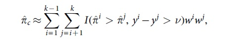
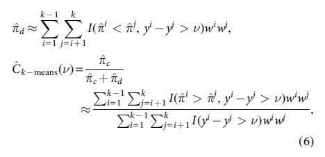
In survival analysis, for example, it can happen that some observations are right censored. To have a comparable pair of two survival times with their predictions, one needs to be sure that the observation with the smallest observed survival time is not censored.^16,17 For the k-means approximation, this can be obtained by adding in the indicator functions of Equation (6) the condition that y_j is not censored.

The implementations of the discussed approximations of the concordance probability are written in R and are available on github as an R-package^†.

Footnotes

Authors' Contributions

All authors contributed to methodology and validation. R.V.O. and J.P. were responsible for conceptualization, formal analysis, investigation, software, and writing (original draft). B.B. and T.V. were responsible for funding acquisition, supervision, and writing (review and editing).

Author Disclosure Statement

No competing financial interests exist.

Funding Information

This work was supported by the Allianz Research Chair Prescriptive business analytics in insurance at KU Leuven and the International Funds KU Leuven under Grant C16/15/068.

Abbreviations Used

Appendix

References

Steyerberg

, Vickers

, Cook

, et al. Assessing the performance of prediction models: A framework for some traditional and novel measures. Epidemiology (Cambridge, Mass.), 2010; 21(1):128.

Liu

X-Y

, Wu

, Zhou

Z-H

. Exploratory undersampling for class-imbalance learning. IEEE Trans Syst Man Cybern Part B (Cybernetics), 2008; 39(2):539–550.

Razavian

, Blecker

, Schmidt

, et al. Population-level prediction of type 2 diabetes from claims data and analysis of risk factors. Big Data, 2015; 3(4):277–287.

De Cnudde

, Ramon

, Martens

, et al. Deep learning on big, sparse, behavioral data. Big Data, 2019; 7(4):286–307.

Bamber

The area above the ordinal dominance graph and the area below the receiver operating characteristic graph. J Math Psychol, 1975; 12(4):387–415.

Reddy

, Aggarwal

. Healthcare Data Analytics, vol. 36. CRC Press: Boca Raton, FL; 2015.

Pencina

, D'Agostino

. Overall C as a measure of discrimination in survival analysis: Model specific population value and confidence interval estimation. Stat Med, 2004; 23(13):2109–2123.

Yan

, Greene

. Investigating the effects of ties on measures of concordance. Stat Med, 2008; 27(21):4190–4206.

Heller

, Mo

. Estimating the concordance probability in a survival analysis with a discrete number of risk groups. Lifetime Data Anal, 2016; 22(2):263–279.

10.

Bouckaert

RR.

Efficient AUC learning curve calculation. In: AI 2006: Advances in Artificial Intelligence. AI 2006. Lecture Notes in Computer Science, vol 4304. (Sattar A, Kang BH. eds.) Springer: Berlin, Heidelberg; 2006; pp. 181–191.

11.

Komori

A boosting method for maximization of the area under the ROC curve. Ann Inst Stat Math, 2011; 63(5):961–979.

12.

Eguchi

, Copas

. A class of logistic-type discriminant functions. Biometrika, 2002; 89(1):1–22.

13.

, Huang

. Regularized roc method for disease classification and biomarker selection with microarray data. Bioinformatics, 2005; 21(24):4356–4362.

14.

Calders

, Jaroszewicz

Efficient AUC optimization for classification. In: Knowledge Discovery in Databases: PKDD 2007. PKDD 2007. Lecture Notes in Computer Science, vol 4702. (Kok JN, Koronacki J, Lopez de Mantaras R et al. eds.) Springer: Berlin, Heidelberg; 2007; pp. 42–53.

15.

Fawcett

An introduction to roc analysis. Pattern Recogn Lett, 2006; 27(8):861–874.

16.

Harrell

, Califf

, Pryor

, et al. Evaluating the yield of medical tests. J Am Med Assoc, 1982; 247:2543–2546.

17.

Gerds

, Schumacher

. Efron-type measures of prediction error for survival analysis. Biometrics, 2007; 63:1283–1287.

18.

Animesh. Predict click through rate (CTR) for a website. 2019. Available from: https://www.kaggle.com/animeshgoyal9/predict-click-through-rate-ctr-for-a-website [Last accessed: September 25, 2020].

19.

GoogleCloud. New york city taxi fare prediction. 2018. Available from: https://www.kaggle.com/c/new-york-city-taxi-fare-prediction [Last accessed: October 1, 2020].

20.

van Breemen

A. N

YC taxi fare—Data exploration. 2018. Available from: https://www.kaggle.com/breemen/nyc-taxi-fare-data-exploration [Last accessed: October 1, 2020].