Hybrid Generalized Regularized Extreme Learning Machine Through Gradient-Based Optimizer Model for Self-Cleansing Nondeposition with Clean Bed Mode of Sediment Transport

Abstract

Sediment transport modeling is an important problem to minimize sedimentation in open channels that could lead to unexpected operation expenses. From an engineering perspective, the development of accurate models based on effective variables involved for flow velocity computation could provide a reliable solution in channel design. Furthermore, validity of sediment transport models is linked to the range of data used for the model development. Existing design models were established on the limited data ranges. Thus, the present study aimed to utilize all experimental data available in the literature, including recently published datasets that covered an extensive range of hydraulic properties. Extreme learning machine (ELM) algorithm and generalized regularized extreme learning machine (GRELM) were implemented for the modeling, and then, particle swarm optimization (PSO) and gradient-based optimizer (GBO) were utilized for the hybridization of ELM and GRELM. GRELM-PSO and GRELM-GBO findings were compared to the standalone ELM, GRELM, and existing regression models to determine their accurate computations. The analysis of the models demonstrated the robustness of the models that incorporate channel parameter. The poor results of some existing regression models seem to be linked to the disregarding of the channel parameter. Statistical analysis of the model outcomes illustrated the outperformance of GRELM-GBO in contrast to the ELM, GRELM, GRELM-PSO, and regression models, although GRELM-GBO performed slightly better when compared to the GRELM-PSO counterpart. It was found that the mean accuracy of GRELM-GBO was 18.5% better when compared to the best regression model. The promising findings of the current study not only may encourage the use of recommended algorithms for channel design in practice but also may further the application of novel ELM-based methods in alternative environmental problems.

Introduction

Sediment transport analysis is required in urban infrastructure hydraulic design. To design drainage and sewer pipes, sedimentation problems should be addressed. Thus, channels are planned to reduce sediment deposition based on various effective parameters. Self-cleansing is a term used in channel design to encompass two basic sediment motion and nondeposition requirements.¹ The nondeposition theory includes three criteria of nondeposition with clean bed, incipient deposition, and nondeposition with deposited bed. The nondeposition with a clean bed criterion is determined by adjusting a velocity or shear stress to satisfy a clean bed channel.^2,3 The incipient deposition is the moment when suspended particles start to deposit. The phenomenon could be set at some area of the channel bed, free of a deposited layer. For the nondeposition with deposited bed concept applicable for large-channel design, an acceptable deposited bed depth is used to decrease the cost of channel construction..^4,5

Nondeposition sediment transport equations were recommended in recent decades to satisfy nondeposition requirements by adjusting limiting velocity or sediment concentration. Pedroli⁶ reported that the sediment size had a significant impact on sediment transport rate. Suspended sediment transport under nondeposition condition was studied by Macke,⁷ Arora,⁸ Nalluri, and Spaliviero.⁹ Detailed experimental studies were conducted on bed load sediment transport and indicated that the design velocity increased with an increase in the pipe size Ab Ghani.¹⁰ May et al,¹¹ De Sutter et al,¹² and Butler et al¹³ analyzed the efficiency of previously suggested equations for the sewer design. Vongvisessomjai et al¹⁴ tested the Camp method in sewer design and demonstrated its significant overestimation for flow velocity computation.

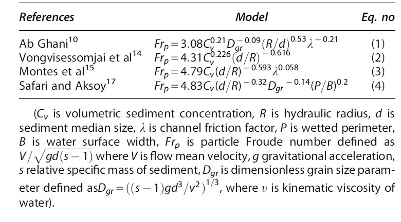
Safari et al³ performed tests in a trapezoidal channel and utilizing own experimental data together with data comprising different sources, recommended a model in which a channel shape factor was embedded based on flow resistance consideration. Montes et al¹⁵ carried out experiments in a large pipe and evaluated their developed model in contrast to the existing counterparts. Safari¹⁶ performed experiments in rectangular, V-bottom, U-shape, trapezoidal, and circular channels for determination of nondeposition mode of sediment transport. Utilizing Safari¹⁶ data, Safari and Aksoy¹⁷ suggested a self-cleansing design model using a simple shape factor applicable for variety of channel shapes. Selected classical regression models are given in Table 1.

Table 1.

Empirical regression equations for nondeposition with clean bed mode of sediment transport

Variety of machine learning techniques were used in open channel sediment transport models. For example, Ab Ghani and Azamathulla¹⁸ tested gene expression programming and uncertainty analysis in sediment transport models. Azamathulla et al¹⁹ implemented adaptive neuro fuzzy inference system (ANFIS) in sediment transport modeling and demonstrated its superiority when compared to the typical regression methods.

Recently, various machine learning techniques, for example, support vector machine (SVM) and extreme learning machine (ELM), SVM-Wavelet, SVM-firefly algorithm, decision tree-artificial neural network (DT-ANN), neuro-fuzzy-based group method of data handling, combination of evolutionary algorithm and ANN, evolutionary polynomial regression, generalized structure group method of data handling, and invasive weed optimization-based ANFIS were attempted to improve sediment transport model performance by Roushangar and Ghasempour,²⁰ Ebtehaj et al,²¹ Ebtehaj et al,²² Ebtehaj et al,²³ Najafzadeh and Bonakdari,²⁴ Ebtehaj and Bonakdari,²⁵ Roushangar and Ghasempour,²⁶ Najafzadeh et al,²⁷ Safari et al,²⁸ and Safari et al,²⁹ respectively. The above-mentioned studies utilized limited number of data, which can be considered as their main deficiency. As can be seen in the studies mentioned above, hybrid algorithms show superior performance in modeling compared to standalone algorithms.

Recently, ELM technique became popular in modeling studies for variety of environmental problems.^30–33 ELM is easy to use and various analytical solutions could be integrated in its algorithm.^34–40 Deo and Şahin⁴¹ investigated the drought index using ELM and ANN. They illustrated the outperformance of ELM in contrast to the ANN by means of model precision and speed. They indicated that ELM is much more faster than the ANN. Online sequential extreme learning machine (OS-ELM) was utilized by Yadav et al³⁴ for flood forecasting. They showed that OS-ELM was superior to genetic programming, ANN and SVM. As an alternative ELM method, Shamshirband et al⁴² implemented kernel extreme learning machine for global solar radiation modeling. They indicated that KELM performed better than support vector regression.

Roushangar and Shahnazi⁴³ implemented wavelet-KELM for estimation of sediment transport with three different scenarios. Inaba et al⁴⁴ introduced generalized regularized extreme learning machine (GRELM), which is a method that makes robust to outlier. They stated that the computing time of the method is less⁴⁵ in contrast to the ELM. One of the main advantages of the GRELM method is that, there is no need to determine the optimal number of neurons. This method reduces the number of neurons to the optimum for initial conditions if the number of neurons is large enough.⁴⁴

This study has three main research contributions. First, this study promotes the sediment transport modeling through implementation of six algorithms of ELM and GRELM coupled with particle swarm optimization (PSO) and gradient-based optimizer (GBO) for the first time in open channel hydraulics. The weight and bias values of the ELM and GRELM methods are hybridized with the novel GBO algorithm and compared with the traditional PSO algorithm performance.

Second, the validity of a design model is related to the range of data used for the model development. While majority of the studies utilized narrow data range, in this study, for the sake of enhancing the validity of the models, wide data ranges collected from different channel cross-sectional shapes were utilized. This is the first implementation of such a large number of experimental data for developing machine learning-based sediment transport models. Furthermore, a data preprocessing analysis to identify the most representative data split samples. Third, effective variables involved in sediment transport hydraulics were incorporated into the model's structure where a channel shape factor is considered in the machine learning-based sediment transport modeling.

Methodology

Experimental data

Experimental laboratory data reported by Mayerle,⁴⁶ May,⁴⁷ Ab Ghani,¹⁰ Vongvisessomjai et al,¹⁴ Safari,¹⁶ and Montes et al¹⁵ are used in this study. Mayerle⁴⁶ carried out tests in two cross-sectional shapes as circular and rectangular. The circular PVC channel had a 20.5 m length and 152 mm diameter. One channel of rectangular had 12.2 m length and 311 mm width and, the other one had 12.6 m length and 462 mm width. Six different granular material sizes with range of 0.5–8.74 mm were utilized in the tests. May⁴⁷ performed tests in a circular pipe with 21.3 m length and 450 mm diameter. Granular material with 0.73 mm size was utilized in the tests.

Ab Ghani¹⁰ performed tests in three channels having circular cross-section shape with diameters of 154, 305, and 405 mm, where 154 and 305 mm diameter pipes had 20.5 m length and 405 mm diameter channel had 21.3 m length. In experiments for channel of 405 mm diameter, granular material size of 0.72 mm and, for 154 and 305 mm diameter pipes, six granular material sizes ranging from 0.46 to 8.3 mm were used. Vongvisessomjai et al¹⁴ performed tests in two channels having diameters of 150 mm and 100 mm, and 16 m length. Three different granular materials having sizes 0.2–0.43 mm were used in the experiments. Further information about these experimental data can be found in Safari et al.^1,28

Novel experimental data of Safari¹⁶ and Montes et al¹⁵ are used in this study, simultaneously, for the first time in the relevant literature. Safari¹⁶ conducted experiments in five cross-sectional shapes: circular, rectangular, trapezoidal, V-bottom, and U-shape channels with length of 12 m. These cross-sectional shapes had approximately width of 300 mm. Four granular materials having median sizes of 0.15–1.52 mm were used. Montes et al¹⁵ conducted tests in a pipe with 595 mm diameter and 10.5 m length. Granular materials with sizes ranging of 0.35–2.60 mm were used in the experiments. List of data sources are given in Table 2.

Table 2.

The datasets used in this study

Reference	Channel shape	Number of data
Mayerle⁴⁶	Rectangular W = 462.3 mm	66
	Rectangular W = 311.5 mm	39
	Circular D = 152 mm	104
May⁴⁷	Circular D = 450 mm	26
Ab Ghani¹⁰	Circular D = 154 mm	39
	Circular D = 305 mm	54
	Circular D = 450 mm	17
Vongvisessomjai et al¹⁴	Circular D = 100 mm	13
Vongvisessomjai et al¹⁴	Circular D = 150 mm	14
Safari¹⁶	Trapezoidal W = 300 mm	25
	Rectangular W = 300 mm	28
	Circular D = 290 mm	25
	U-shape W = 300 mm	25
	V-bottom W = 300 mm	21
Montes et al¹⁵	Circular D = 595 mm	107
Total		603

D is circular channel diameter.

Extreme learning machine

Having single-layer feedforward neural network (SLFN), ELM was suggested by Huang et al.⁴⁸ ELM is a learning algorithm that creates input weights at random and analyzes the SLFN output weights.⁴⁹ The advantages of ELM include better performance, learning speed, applicability, and competence for several types of activation and kernel functions.^50–52 It could be shown that ELM includes integrated radial basis function (RBF) and hidden nodes through:

in which β_i is the weight of the ith hidden and output nodes, w_i and b_i indicate the hidden nodes learning variables (weights and bias) and L is the hidden nodes number. $H (w_{i}, b_{i}, x)$ is the output function of ith hidden nodes related to the input value of x defined as $H (w_{i}, b_{i}, x) = g (w_{i} \cdot x + b_{i}), b_{i} \in R$ (6)

in which g(x) denotes the activation function type, for instance, sigmoid, radial basis, hardline, and so on. Here, g(x) refers to the radial basis activation function that could be written as follows: $H (w_{i}, b_{i}, x) = g (b_{i} | | x - w_{i} | |), b_{i} \in R^{+}$ (7)

in which w_i and b_i denote the center and impact factor of ith RBF node. Eq. (7) can be expressed as below: $H β = T$ (8)

in which $H (w, b, x) = {(\begin{matrix} H (w_{1}, b_{1}, x_{1}) & \dots & H (w_{L}, b_{L}, x_{1}) \\ ⋮ & ⋱ & ⋮ \\ H (w_{1}, b_{1}, x_{N}) & \dots & H (w_{L}, b_{L}, x_{N}) \end{matrix})}_{N \times L}$ (9)

where T denotes the training target matrix and H is ELM's hidden layer output matrix. The adjustment of the output values to the target values (T) was achieved by editing the output weights as $β = H^{T} T$ (10)

Output weights (β) were calculated with H^T that is a Moore–Penrose generalized inverse matrix of ELM's hidden layer output. In the present study, hidden layer number of neurons was adjusted as 30 through a trial and error procedure and, as an activation function, RBF was used in the ELM model framework. The architecture of the ELM is depicted in Figure 1.

FIG. 1.

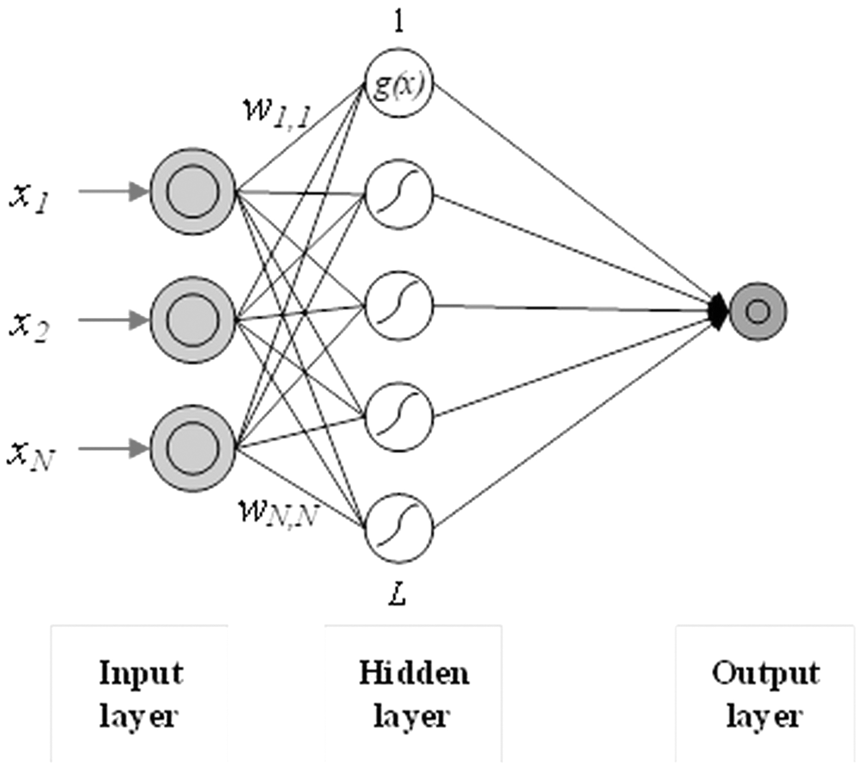
The general ELM structure. ELM, extreme learning machine.

Generalized regularized extreme learning machine

Alternative generation of ELMs were developed that are more compatible with various data types by editing classic ELM weights,^53,54 loss,^55,56 and activation functions.^37,49,57 Deng et al⁵³ introduced the weighted regularized ELM through including a positive quantity in the $H^{T} H$ or $H H^{T}$ diagonal to achieve a robust result and enhancing its generalization efficiency. They suggested the following equations for minimization⁵³: $H β - y = δ$ (11) ${minimize}_{β} ∥ β ∥_{1} + λ_{2} ∥ β ∥^{2}$ (12)

in which ϵ denotes the error vector, C regularization variable, is the connection of M hidden layer neurons and D denotes a diagonal weight matrix for outlier performance promotion. Deng et al⁵³ included the sigmoid additive type of SLFN in the performance analysis.

To analyze the output weights, Martínez-Martínez et al⁵⁸ emphasized various penalties for least squares regression. Variety types of penalties such as Lasso, ridge regression, and elastic nets^59–61 were studied in the regularization. The three regularization methods were generally defined as $(β_{0}, β) \in ℛ^{N^{\sim} + 1}$ :

in which λ denotes the regularization variable, the $h_{k}^{T}$ is kth row of the matrix H, $P_{α}$ denotes a balance for ridge regression penalty ( $α = 0$ ), and lasso penalty ( $α = 1$ ).⁵⁸

Wang et al⁶² were the first authors who investigated generalized ELM (GELM).⁶³ Output weights are fixed in the classical ELM and unrelated to the sample inputs. When compared to ELM, GELM applies p-order reduced polynomial functions for all input features as output weights. More willingly than using R-ELM, to each T value, they searched for jointly sparse solutions. The motivation was to determine a solution with common nonzero support that would reveal a compact network (Fig. 2). The GRELM method is implemented in R-ELM for multiclass classification problems. GRELM uses alternating direction method of multipliers⁶⁴ for solving the Eq. (14):

FIG. 2.

The general GRELM structure. GRELM, generalized regularized extreme learning machine.

{minimize}_{B} \frac{C}{2} ∥ H B - T ∥_{F}^{2} + λ_{1} ∥ B ∥_{2, 1} + \frac{λ_{2}}{2} ∥ B ∥_{F}^{2},

(14)

in which $∥ . ∥_{F}$ denotes the Frobenius norm, $| | B | |_{2, 1} = \sum_{i = 1}^{M^{\sim}} | | b_{i, \cdot} | |$ , (ℓ_2,1 norm) and $b_{i, \cdot}$ denotes the ith row of B. Thus, GRELM offers faster and more compact solutions by eliminating the ELM neurons. Also, it was reported that GRELM leads to better results with high neuron numbers or when the data set is complex. Further information can be found in Inaba et al.⁴⁴ In this study, GRELM parameters, the hidden layer neuron count, regularization parameter, and norms contribution balance were selected as 90, 9000 and 0.6, respectively.⁶⁵

Particle swarm optimization

PSO algorithm is a swarm intelligence method. Eberhart and Kennedy⁶⁶ developed this approach for optimizing difficult engineering problems by utilizing members of a population known as particles, which they named the particle algorithm. In each generation, the particle positions are updated by applying a set of velocity vectors to the current values. While the optimization process is in progress, each particle regulates its location in relationship to its own experience and that of the optimal experience. During each generation, the position and velocity of each particle is determined by Eqs. (15) and (16): $v_{k, i}^{n e w} = w \times v_{k, i} + c_{1} \times r_{1} \times (x p_{k, i} - x_{k, i}) + c_{2} \times r_{2} \times (x g - x_{k, i})$ (15) $x_{k, i}^{n e w} = x_{k, i} + v_{k, i}^{n e w}$ (16)

where k represents particle of the movement, $v_{k, i}$ is velocity of the particle, and $x_{k, i}$ is their position at the current generation. $x p_{k, i}$ is the best position of the particle, xg is the most advantageous position in the swarm. The new index indicates the next generation.

Therefore, $v_{k, i}^{n e w}$ and $x_{k, i}^{n e w}$ are the updated velocity and position of the particle. Together with the random vectors r₁ and r₂ within the range [0, 1] and the acceleration coefficients c₁ and c₂ within the range [0, 2] determine the stochastic influence of cognitive and social components on the overall velocity of a particle. w is the inertia weight within the range [0.5, 0.9].

Gradient-based optimizer

Metaheuristic algorithms are inspired by nature or basic principles. GBO, which is one of the metaheuristics, was developed using Newton's approaches by Ahmadianfar et al.⁶⁷ First, GBO method is started by selecting initialize parameters, which includes number of iterations and the population size depending on the problem complexity. In GBO, the vector of N vectors in D-dimensional space can be described. Each member of the population indicates vector (X_m) in GBO. To initialize, N vectors with D dimensionally are created as follows: $x_{m} = L B + r a n d \times (U B - L B)$ (17)

where LB and UB are lower boundary and upper boundary in problem definition, respectively. rand is the random vector within range [0, 1].

Second, the GBO algorithm searches feasible space using gradient search rule approach. The GSR regulates vector movement to improve search within the feasible domain and reach better placements. The GSR method is suggested with the goal of increasing the exploration tendency and accelerating the convergence of the GBO. It is based on the notion of the GB method. This rule, however, is derived from Newton's gradient-based technique. The GSR is expressed as follows: $G S R = r a n d n . R_{1} . \frac{2 Δ x \times x_{m}}{(x_{w o r s t} - x_{b e s t} + ε)}$ (18) $x_{w o r s t} = r a n d . (\frac{[u_{m + 1} + x_{m}]}{2} + r a n d . Δ x)$ (19)

x_{b e s t} = r a n d . (\frac{[u_{m + 1} + x_{m}]}{2} - r a n d . Δ x)

(20)

u_{m + 1} = x_{m} - r a n d n . \frac{2 Δ x . x_{m}}{(x_{w} - x_{b} + \in)} + G D

(21)

where rand and randn represents random value and the value with a normal distribution, which includes vector of N element. ɛ is a small number within the range of [0, 0.1]. x_worst and x_best are the positions during the optimization process, R₁ is the weighting factor and u_m ₊ ₁ is the new vector generated by updating x_m. The GD is expressed as follows: $G D = r a n d . R_{2} \times (x_{b} - x_{m}^{i t})$ (22)

where R₂ parameter is a random value that enables each vector to have a unique step size. For each iteration, new solutions are obtained using GSR, GD, and x_m. Finally, the GBO uses local escaping operator to tackle complicated issues. This operator can dramatically alter the position of solution.⁶⁸

Hybridization process

In this study, ELM and GRELM standalone models was applied to determine best model for sediment transport. Then, ELM and GRELM hybridized with PSO and GBO. Therefore, four hybrid algorithms, ELM-PSO, ELM-GBO, GRELM-PSO, and GRELM-GBO were utilized for prediction of particle Froude number in open channel. Node parameters of the ELM and GRELM, biases and weights were optimized using root mean square error (RMSE) as fitness function. Table 3 indicates PSO and GBO parameters. Figure 3 displays flowchart of PSO and GBO. The hybrid models results were examined in terms of performances and finally the best model is introduced as the superior model for particle Froude number computation.

FIG. 3.

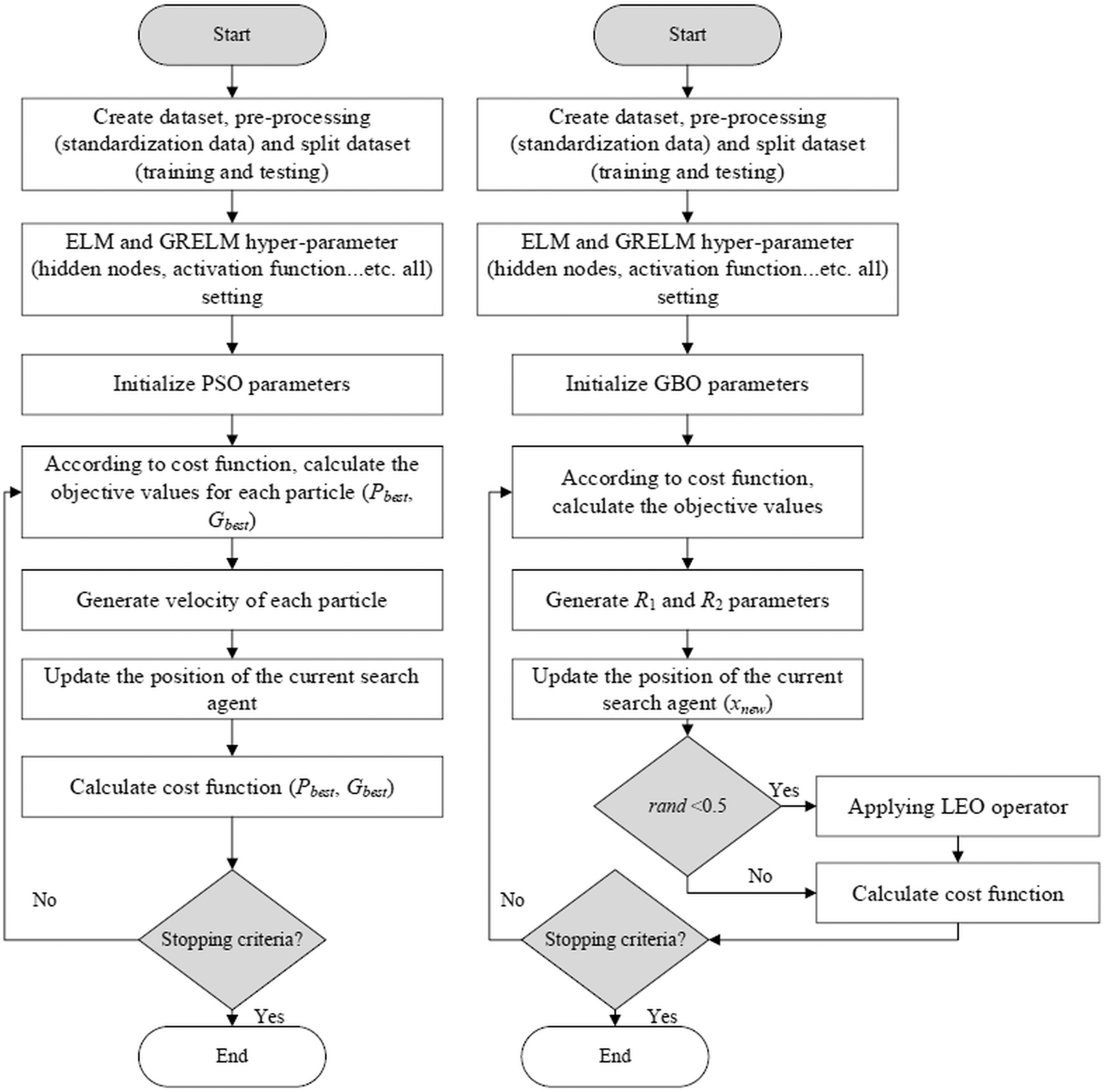
The flowchart of PSO and GBO. GBO, gradient-based optimizer; PSO, particle swarm optimization.

Table 3.

The initial parameters of particle swarm optimization and gradient-based optimizer evolutionary algorithms

GBO	PSO parameters
Number of positions = 200	Personal learning coefficient (c₁) = 0.09
Maximum iteration = 1000	Global learning coefficient (c₂) = 2
Search range = [−1 1]	Inertia weight (w) = 0.1
	Inertia weight damping ratio = 0.89
	Maximum iteration = 1000
	Population = 100
	Search range = [−1 1]

GBO, gradient-based optimizer; PSO, particle swarm optimization.

Performance criteria

The analysis of model performance is important in investigating the credibility of the models. Thus, RMSE, root mean square difference (RMSD), mean absolute error (MAE), mean absolute relative error (MARE), BIAS, and coefficient of determination (R²) were used in this study to determine the goodness-of-fit index. The model performs well with R² close to the unity, and RMSE, MAE, and MARE close to zero. The RMSE, MAE, MARE, BIAS, and R² could be computed, using the below equations, respectively:

where, y_j is the observed value, ŷ_j is the predicted value, subscript of m indicates the mean value, and n is the data number.

Results

Data preparation

Effective self-cleaning models use flow, fluid, and sediment characteristics.¹ Within the structure of self-cleansing sediment transport models, sediment volumetric concentration (C_v) or particle Froude number is used as dependent parameter as functions of other effective parameters. Relaying on the relevant literature, flow velocity (V), gravity acceleration (g), hydraulic radius (R), fluid-specific mass (ρ), fluid kinematic viscosity (υ), sediment volumetric concentration (C_v), median size of sediment (d), channel friction factor (λ), and sediment relative specific mass (s) could be considered as effective sediment transport variables for the modeling. Furthermore, P/B as a cross-section shape factor can be used to express the channel shape properties for generalization of the developed model.¹⁷ Taking into account of aforementioned variables, as s group of dimensionless parameters, following expression is written.

where D_gr is the dimensionless grain size parameter as $D_{g r} = {(\frac{(s - 1) g d^{3}}{v^{2}})}^{1 ∕ 3}$ (30)

Statistical characteristics of the utilized data are listed in Table 4. In the current study, data split rates of 70% and 30% were applied to the whole data for training and testing stages, respectively. Based on the results reported by Ebtehaj et al,⁶⁹ who conducted uncertainty analysis, it was indicated that the split between training and testing data would not make a significant difference in model performance; however, the best data split rate was reported as 70% and 30% during the training and testing stages, respectively.

Table 4.

Statistical properties of the entire data

	Range	Mean	SD	Skewness	Kurtosis
C_v	1 × 10⁻⁶–0.02	8.73 × 10^–4	0.0019	5.72	43.53
D_gr	3.76–221.09	50.75	53.02	1.77	5.57
d/R	0.0034–0.41	0.06	0.07	2.12	8.63
λ	0.0036–0.17	0.03	0.015	3.14	22.83
P/B	1.01–2.79	1.32	0.31	1.96	7.45
Fr_p	1.29–16.07	5.13	2.63	0.99	3.81

SD, standard deviation.

Determination of the best data distribution

The distribution of training and testing data affects the machine learning modeling results. Inappropriate training and testing data discriminations may cause to overfitting or underfitting problems. In the present study, laboratory data taken from six different sources were compiled. The utilized data sets included the widest data range in the literature. An accurate sediment transport model should fit the best-fit line to avoid underestimation or overestimation problems. Otherwise, a lower learning status would prevent a safe infrastructure planning. Similarly, overestimation problem would lead to a noneconomic model. Considering these problems, the dataset was determined to include 10 random distributions based on 70% for training and 30% for testing distributions. The statistics of the data distributions are presented in Figure 4.

FIG. 4.

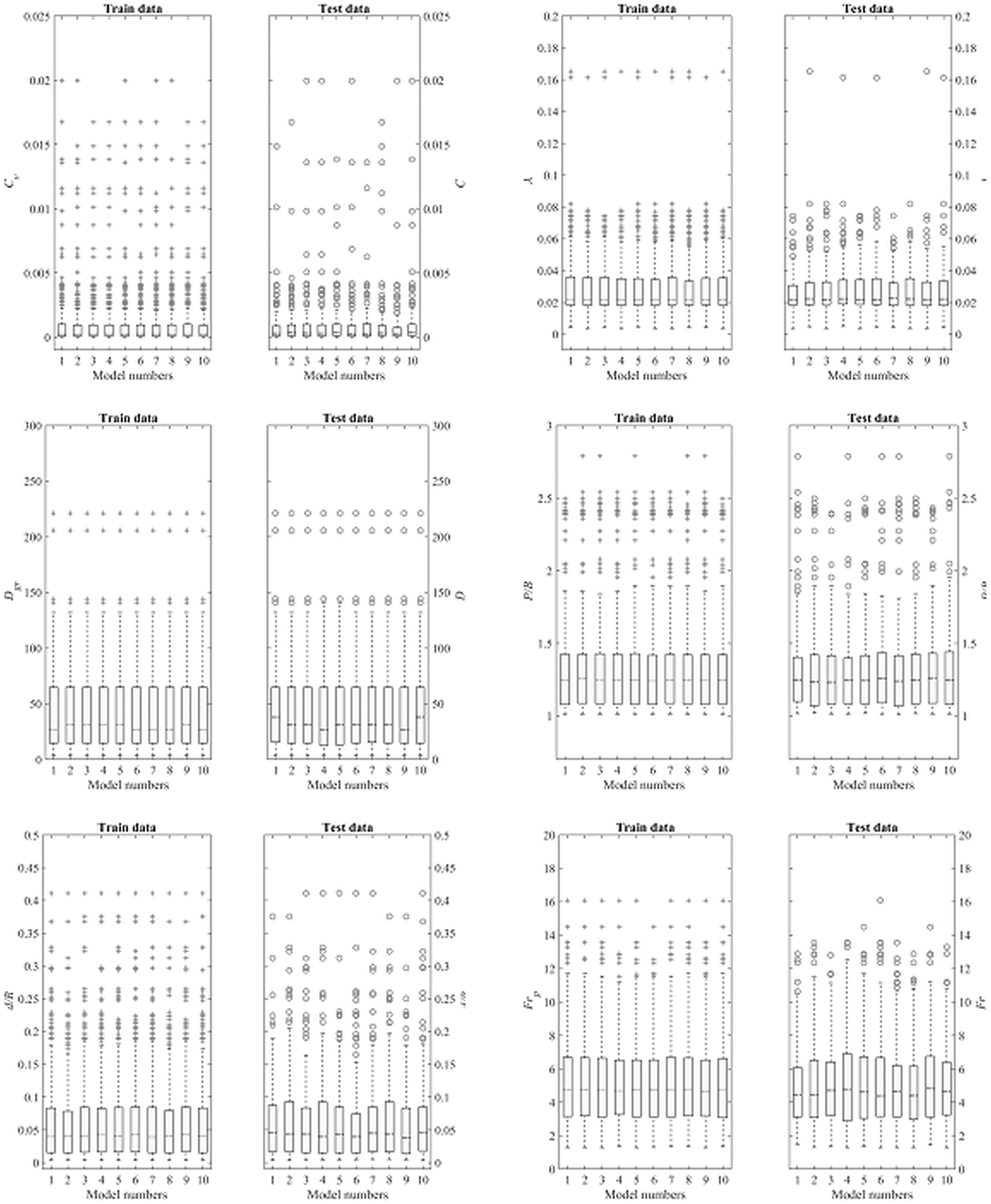
Boxplots for different data splits at training and test stages.

In previous studies conducted with a smaller data range, it was reported that C_v was the most effective parameter. On the contrary, outliers affect the performance of the machine learning methods. As seen in Figure 4, the outlier count was quite higher for the C_v input. This is because of the quite wide data range. It was suggested to remove the outliers and data noise to improve the machine learning performance. However, it is impossible for the experimental data used in this study.

The utilized data were divided into 10 different sections as training and testing splits. The boxplots presented in Figure 4 consist of five sections; minimum and first (q₁), median and third (q₃) quartiles, and maximum. Points other than those specified exhibit outliers (O). In the present study, maximum whisker length (w) was selected as 1.5. Outlier initial value was calculated using Eq. (31): $O_{i} = q_{3} + w (q_{3} - q_{1}) i \in R^{m}$ (31)

where m indicates the model number and q is quartile of data. Positive skewness could be observed in Table 3 and Figure 4. Standardization of the data was conducted between [−1 1] applying the below relationship. $y = \frac{2 \times (x - x_{min})}{x_{max} - x_{min}} - 1$ (32)

Utilizing the randomly selected 10 different data distributes, ELM and GRELM models were developed. The results are given in Table 5 for 10 different data split scenarios. The performances of two models developed in this study, namely ELM and GRELM, were compared based on various statistical error measurement criteria, including R², RMSE, MAE, BIAS, and MARE, as shown in Table 5 for the training and testing phases, separately. Results indicated that GRELM was superior to ELM in all models. Training performance results are important in machine learning techniques where a model could have overfitting or underfitting problems. These problems are solved during the training and testing stages. ELM could also lead to overfitting problems, especially for higher number of neurons. To tackle this problem, the most suitable hidden neurons number is determined by choosing the model where the training and testing performances were almost the same.

Table 5.

Performance of extreme learning machine and generalized regularized extreme learning machine models for different data distributions

Phase	Model	Training					Testing
Split	Model	R²	RMSE	MAE	BIAS	MARE	R²	RMSE	MAE	BIAS	MARE
1	ELM	0.83	1.11	0.78	0.0001	0.16	0.75	1.20	0.87	0.0444	0.20
1	GRELM	0.89	0.90	0.63	0.0000	0.13	0.78	1.12	0.84	0.0127	0.19
2	ELM	0.75	1.28	0.90	0.0002	0.20	0.77	1.32	0.94	−0.1163	0.20
2	GRELM	0.80	1.16	0.82	0.0000	0.18	0.79	1.28	0.91	−0.0780	0.21
3	ELM	0.81	1.17	0.83	0.0001	0.18	0.78	1.20	0.88	0.0901	0.20
3	GRELM	0.78	1.26	0.87	−0.0018	0.19	0.79	1.15	0.85	0.0693	0.19
4	ELM	0.75	1.23	0.85	0.0007	0.18	0.76	1.44	1.05	−0.0852	0.23
4	GRELM	0.81	1.07	0.74	−0.0490	0.15	0.78	1.39	1.02	0.0282	0.22
5	ELM	0.76	1.23	0.86	−0.0005	0.19	0.76	1.42	1.00	−0.0536	0.20
5	GRELM	0.81	1.10	0.78	−0.0001	0.17	0.79	1.31	0.93	−0.0719	0.20
6	ELM	0.84	1.03	0.73	0.0002	0.16	0.75	1.45	0.96	−0.2576	0.20
6	GRELM	0.86	0.96	0.69	0.0000	0.15	0.76	1.41	0.91	−0.1989	0.18
7	ELM	0.76	1.31	0.90	−0.0002	0.19	0.78	1.22	0.88	0.0766	0.20
7	GRELM	0.81	1.15	0.81	0.0001	0.18	0.82	1.12	0.80	0.0350	0.18
8	ELM	0.77	1.28	0.89	0.0000	0.19	0.77	1.24	0.94	0.1207	0.23
8	GRELM	0.76	1.30	0.91	0.0002	0.20	0.78	1.17	0.89	0.0276	0.20
9	ELM	0.76	1.28	0.89	−0.0004	0.19	0.76	1.30	0.88	0.0255	0.18
9	GRELM	0.81	1.13	0.79	0.0001	0.17	0.78	1.25	0.83	0.0442	0.17
10	ELM	0.78	1.25	0.91	0.0001	0.20	0.75	1.25	0.93	0.0564	0.22
10	GRELM	0.83	1.12	0.79	0.0041	0.17	0.76	1.26	0.90	−0.0626	0.21

ELM, extreme learning machine; GRELM, generalized regularized extreme learning machine; MAE, mean absolute error, MARE, mean absolute relative error; RMSE, root mean square error.

After all, training and testing data ranges are closely related to overfitting or underfitting issues. Especially, in S4 and S6, the training data range is smaller than the testing counterpart for many parameters (Fig. 4). Therefore, S4 and S6 are models with the highest overfitting problem. Training performance was better than test performance in all different scenarios for GRELM. However, for GRELM and ELM, test performances showed better results than training in some scenarios. Considering the data distributions in S8 and S9 in Figure 4, test data ranges are smaller than training data ranges. For all scenarios, the BIAS criterion gave better results in training stage in contrast to the testing outcomes.

As a result of all these indicators, S7 was chosen as the superior model and accordingly, it is selected to compare with classical regression equations. For ELM and GRELM models the rate of change of the RMSE values are found as 20.83% and 25.89%, respectively.

Figure 5 demonstrates the scatter of machine learning methods at the training stage. Outlier initial values for models 1–10 for the training data were O₁ = 12.54, O₂ = 12.06, O₃ = 12.42, O₄ = 11.79, O₅ = 11.89, O₆ = 11.94, O₇ = 12.32, O₈ = 12.43, O₉ = 12.18, and O₁₀ = 12.43, respectively (Fig. 4). Model outliers could be observed especially at the beginning of the scatter. GRELM's outlier performance was better than that of ELM. ELM and GRELM exhibited almost the same trends.

FIG. 5.

Scatter plots for models at training phase.

To provide a practical tool for, the following equations (Eqs 27–28) can be used to determine the Fr_p using the best GRELM-GBO model, where InV is the input variable vector, InW is the input weight, OW is the output weight, and BHN is the bias of hidden neurons as given in Table 6.

Table 6.

The weights and bias values for generalized regularized extreme learning machine gradient-based optimizer model

InW =					OW =	BHN =
[0.756	0.743	0.277	−0.489	−0.608	[−0.467	[0.287
0.740	0.998	−0.692	0.317	0.914	0.385	0.563
0.409	−0.390	−0.584	0.439	0.343	−0.433	0.761
−0.060	−0.459	0.188	−0.855	−0.952	−0.485	0.790
0.267	0.615	0.686	−0.304	0.298	−0.516	−0.074
−0.288	0.330	0.298	−0.185	0.156	−0.299	−0.388
−0.190	0.890	−0.096	−0.844	−0.252	−0.488	0.617
−0.118	0.439	0.297	0.385	−0.205	−0.592	0.899
−0.781	0.494	0.197	−0.161	0.407	1.000	0.833
0.681	0.776	0.683	0.216	−0.359	0.418	0.510
−0.329	−0.290	−0.775	−0.177	−0.300	−1.000	−0.999
−0.292	−0.555	0.974	0.258	0.998	0.685	−0.246
−0.333	−0.652	−0.324	1.000	−0.999	0.236	−0.255
0.463	0.189	0.980	0.079	−0.095	−0.114	0.164
0.165	−0.232	−0.316	0.379	−0.369	−0.153	−0.459
−0.711	−0.229	−0.541	−0.972	−0.567	−0.162	−0.998
−0.999	−0.316	0.363	−0.578	0.409	0.146	−0.908
−0.131	−0.922	0.587	0.329	0.292	0.146	−0.462
−0.109	0.998	0.878	−0.088	0.074	0.637	0.365
0.122	0.237	−0.337	0.339	1.000	−0.231	−0.474
−0.774	−0.862	−0.100	0.340	0.488	−0.749	0.324
0.191	0.155	−0.623	−0.247	−0.034	−0.263	0.476
0.327	0.346	−0.157	0.525	1.000	−0.485	0.291
−0.900	0.188	0.557	0.364	0.113	−0.998	−0.379
0.595	−0.994	0.648	0.522	−0.168	0.580	0.550
0.263	−0.307	−0.848	−0.127	0.491	0.198	0.915
0.256	0.052	−0.400	0.099	0.546	0.556	−0.223
0.994	0.710	−0.105	−0.994	0.241	0.796	−0.899
0.620	−0.821	0.882	−0.487	−0.447	0.146	−0.226
0.471	−0.999	0.149	0.381	0.998	−0.418	−0.091
1.000	0.327	−0.114	0.116	−0.354	−0.377	0.149
−0.687	1.000	−0.998	−0.588	−0.999	0.705	0.905
−0.669	0.213	−0.295	0.200	0.483	0.127	0.157
1.000	0.176	−0.528	0.708	0.504	0.076	0.146
0.393	−0.229	−0.584	0.415	0.461	0.835	0.289
1.000	−0.259	−0.505	−0.365	−0.312	0.988	−0.889
0.198	−0.502	−0.141	0.097	−0.532	−0.684	0.602
−0.494	0.144	0.162	−0.655	−0.081	0.186	0.167
0.370	0.292	0.346	−0.292	0.404	0.262	−0.187
0.673	−0.247	−0.207	−0.080	−0.398	0.837	1.000
0.709	0.974	0.499	0.590	−0.278	−0.440	0.174
0.538	−0.313	0.610	−0.997	−0.609	−0.095	−0.055
−0.132	0.343	−0.804	−0.959	0.585	0.419	−0.999
−0.246	−0.944	0.595	−0.911	0.454	0.243	−0.381
0.128	−0.554	0.460	−0.603	0.999	−0.852	0.530
0.515	0.361	−0.999	−0.187	0.948	0.271	−0.365
0.572	−0.319	−0.477	−0.330	−0.146	0.188	0.109
0.999	−0.621	−0.583	−0.986	0.247	−0.203	−0.319
−0.571	−0.360	−0.255	0.169	0.999	0.920	0.816
0.516	0.321	−0.052	0.525	−0.836	−0.359	−0.552
0.512	−0.802	0.351	0.551	−0.651	0.231	−0.364
−0.580	0.141	−0.726	−0.208	0.843	0.789	−0.545
−0.158	−0.226	0.492	−0.597	0.330	0.500	−0.153
−0.146	0.999	−0.314	−0.035	−0.074	−0.376	0.150
0.880	−0.518	−0.521	−0.996	0.432	−0.254	−0.620
−0.563	−0.092	−0.560	0.280	−0.675	−0.086	−0.554
0.250	−0.737	−0.869	0.676	−0.417	−0.995	−0.935
−0.051	−0.413	−0.928	0.686	0.988	−0.083	0.150
−0.150	−0.252	−0.348	−1.000	0.638	0.314	0.577
−0.495	−0.241	0.953	−0.768	0.601	0.838	−0.159
0.531	−0.184	−0.566	−0.302	0.453	−0.543	0.360
−0.315	0.999	0.201	−0.469	1.000	−0.195	−0.221
−0.131	0.618	−1.000	0.196	0.591	0.130	0.999
−0.241	−0.255	0.094	−0.537	−0.273	0.853	−0.629
0.887	0.310	−0.690	−0.181	−0.489	0.200	−0.203
−1.000	−0.770	0.625	−0.999	0.665	0.543	0.573
0.732	0.381	0.322	0.276	0.107	−0.836	−0.384
−0.510	−0.549	−0.722	0.878	0.023	−0.714	−0.492
−0.079	0.684	0.664	0.460	−0.218	−0.998	−0.998
−0.522	−0.427	0.691	0.199	−0.593	−0.951	−0.557
0.761	0.551	0.679	−0.202	−1.000	0.580	−0.208
−0.237	−0.718	−0.347	0.237	0.419	0.003	−0.853
0.036	−1.000	0.305	0.592	0.364	0.213	0.299
−0.118	0.288	0.999	−0.184	0.493	−0.054	0.564
0.560	0.176	−0.170	−0.872	0.603	−0.590	0.189
0.776	0.295	−0.440	−0.097	−0.989	0.075	−0.413
−0.440	0.226	0.155	0.254	0.040	0.277	−0.062
−0.239	−0.292	0.624	−1.000	0.968	−0.185	0.126
−0.340	0.130	−0.677	0.210	0.258	−0.190	0.501
−0.109	0.645	0.755	0.515	0.885	0.095	0.828
−0.527	−0.672	−1.000	−0.570	0.224	0.389	0.223
0.156	0.692	0.181	0.419	−0.559	−0.417	−0.571
0.459	−0.235	0.223	−0.829	0.266	0.361	−0.999
−0.055	0.337	−0.172	−0.305	0.495	−0.238	0.261
−0.999	−0.277	0.343	0.922	0.480	0.218	−0.104
−0.999	−0.363	0.600	−0.959	0.560]	−0.196]	0.475]

F r_{p} = {[\frac{1}{(1 + exp (I n I W \times I n V + B H N))}]}^{T} \times O W

(27)

ln V = [\begin{matrix} C_{v} \\ D_{g r} \\ d ∕ R \\ λ \\ P ∕ B \end{matrix}]

(28)

Comparison of hybridized ELM and GRELM with classical benchmarks

Statistical comparison of ELM, ELM-PSO, ELM-GBO, GRELM, GRELM-PSO, and GRELM-GBO as machine learning algorithms and conventional regression equations of Ab Ghani,¹⁰ Vongvisessomjai et al,¹⁴ Montes et al¹⁵ and Safari, and Aksoy¹⁷ is listed in Table 7 by means of R², RMSE, MAE, BIAS, and MARE. Results show that ELM, ELM-PSO, ELM-GBO, GRELM, GRELM-PSO, and GRELM-GBO outperform all empirical regression equations although, Safari and Aksoy¹⁷ is superior to the other classical regression equations. GRELM-GBO provided best results with lowest error and higher correlation. Since GRELM-GBO had positive BIAS values, it produced slight overestimation. GRELM-GBO improved the best regression equation by a factor of 18.5%. Figure 6 illustrates the scatter plots for ELM, ELM-PSO, ELM-GBO, GRELM, GRELM-PSO, GRELM-GBO, and conventional regression equations. As seen in Figure 6, all machine learning models and conventional regression equations were distributed for outlier values.

FIG. 6.

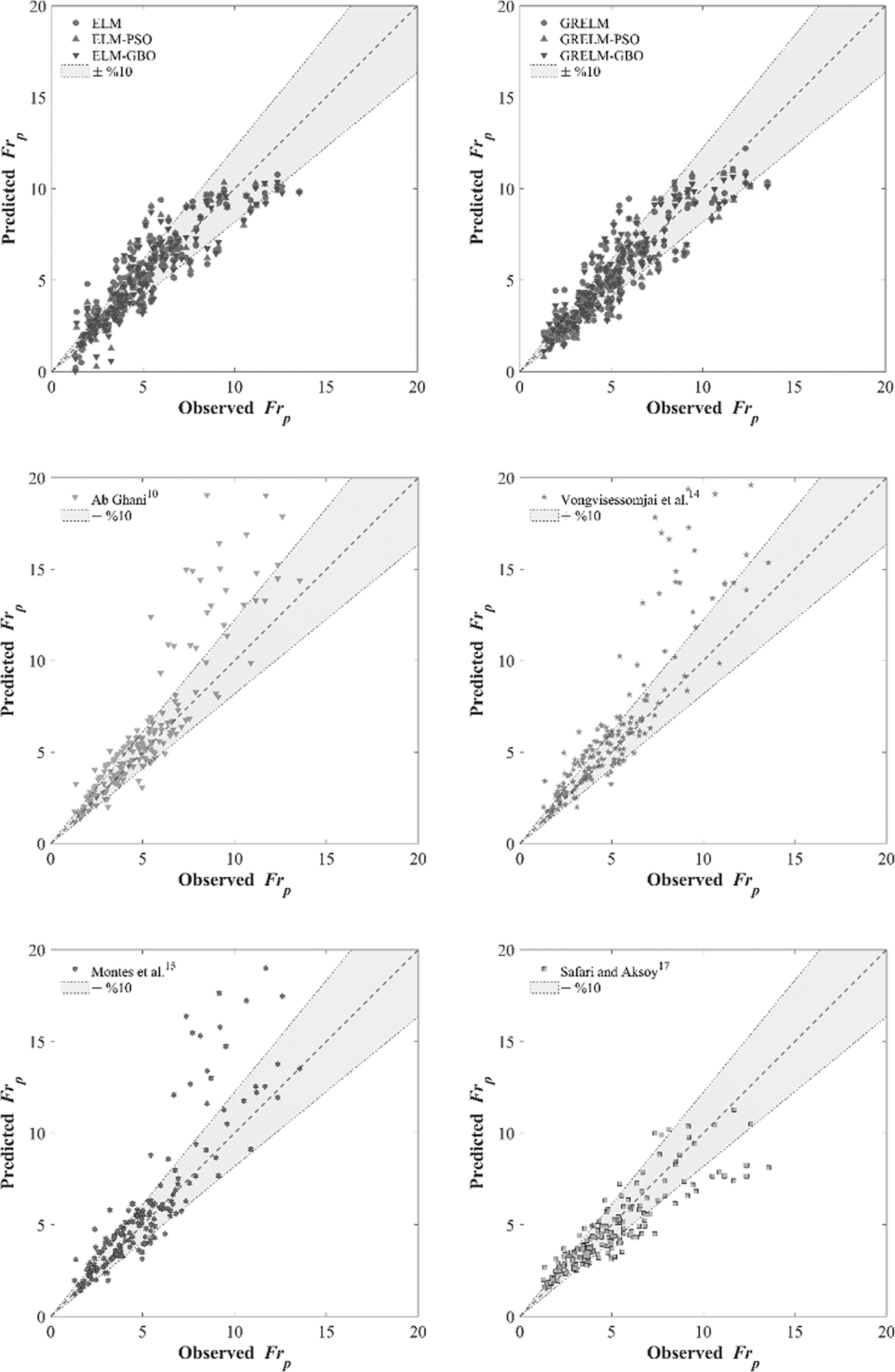
Scatter plots for machine learning and empirical regression equations at testing stage.

Table 7.

Comparison of models for best distribution (S7)

	R²	RMSE	MAE	BIAS	MARE
Training
ELM-PSO	0.80	1.20	0.83	−0.0051	0.17
ELM-GBO	0.81	1.15	0.81	−0.0068	0.17
GRELM-PSO	0.81	1.17	0.82	0.0026	0.17
GRELM-GBO	0.81	1.14	0.80	−0.0076	0.17
Testing
ELM	0.78	1.22	0.88	0.0766	0.20
ELM-PSO	0.81	1.12	0.81	0.0662	0.17
ELM-GBO	0.82	1.10	0.80	0.0143	0.17
GRELM	0.82	1.12	0.80	0.0350	0.18
GRELM-PSO	0.83	1.09	0.81	0.0197	0.18
GRELM-GBO	0.84	1.06	0.77	0.0632	0.17
Ab Ghani¹⁰	0.81	2.08	1.19	0.8976	0.22
Vongvisessomjai et al¹⁴	0.79	2.50	1.42	1.1829	0.26
Montes et al¹⁵	0.78	1.96	1.11	0.6727	0.21
Safari and Aksoy¹⁷	0.78	1.30	0.90	−0.3546	0.18

For machine learning models of ELM and GRELM at testing sages for 10 different splits, the initial outliers were O₁ = 11.45, O₂ = 12.63, O₃ = 11.78, O₄ = 13.22, O₅ = 13.01, O₆ = 12.89, O₇ = 12.03, O₈ = 11.73, O₉ = 12.37, and O₁₀ = 11.75 (Fig. 6). When the performances of machine learning algorithms are evaluated, it can be found that GRELM outlier performance is found superior to ELM.

Overestimating and underestimating model performances are common problems in machine learning modeling. For the case of overestimation, the results of the model will be larger than their actual values. This design tool will create economic problems in the planning of engineering structures where channels need higher velocity and accordingly, steeper bed slope. However, underestimation is also the case where the model results are lower than the real value. This problem will cause problems such as early sedimentation and maintenance expenditures. To address these concerns, it is needed to construct a model with minimum underestimation or overestimation. Although Safari and Aksoy¹⁷ model generated slight underestimation, Ab Ghani,¹⁰ Vongvisessomjai et al,¹⁴ and Montes et al¹⁵ models gave a significant overestimation.

Discussion

Determination of the flow velocity required for sewer design is vital in infrastructure engineering. As a design standard, different self-cleansing approaches of nondeposition, incipient deposition, and incipient motion can be implemented. This study concentrates on the nondeposition with clean bed design method. Existing machine learning-based models were established for different cross-section shapes where channel geometrical characteristics were not utilized as a model effective parameter. Overestimation and underestimation of a design model cause for additional expenditures. For example, as described in the previous section, the conventional regression equations underestimate or overestimate particle Froude number in testing phase. Designing a channel that underestimates the expected Froude particle number induces early overflow and sediment deposition, the reverse application of an overestimated model causes a greater velocity and, therefore, a steeper bed slope is needed in channel construction. This study suggests GRELM-GBO, as a novel machine learning method to overcome all these problems.

Classical nonlinear regression approach was widely used to develop models considering the effective parameters involved in nondeposition mode of sediment transport. Several studies have shown a deficit in accurate estimation for certain cross-sectional forms in classical regression methods.^3,17 Toward this, the current study applied ELM, ELM-PSO, ELM-GBO, GRELM, GRELM-PSO, and GRELM-GBO as robust machine learning methods. Although there are many studies in the implementation of ELM, the novel generation of ELM as GRELM algorithm was rarely used in the literature for the environmental problems. Thanks to the ELM compact algorithm, it can be integrated very quickly and easily. To this end, in this study, the GRELM-PSO and GRELM-GBO methods, which are superior to hybridized ELMs, were used to model the nondeposition mode of sediment transport applicable for channel design. Figure 7 illustrates an improvement in machine learning modeling when compared to the best conventional regression equation¹⁷ for all models in testing phase. Percentage improvement (P_i) was calculated using

FIG. 7.

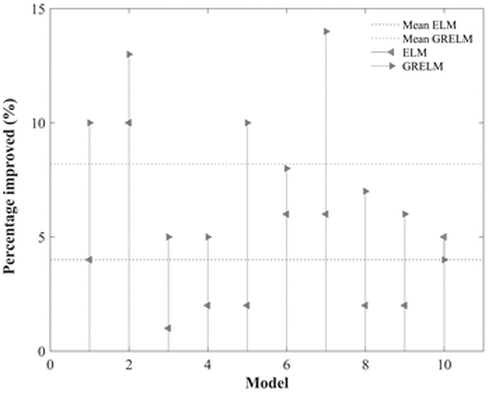
Comparison of the best empirical regression equation (Safari and Aksoy¹⁷) with ELM and GRELM machine learning models.

P i = ((R M S E s - R M S E m) ∕ R M S E s) \times 100

(26)

where RMSEs is RMSE value of the best conventional regression equation¹⁷ and RMSEm is RMSE value of machine learning algorithms. GRELM outperformed ELM based on the percentage improvement. The improvement ranking considering machine learning algorithms did not change for all models. The improvement in GRELM has an average of 15% and GRELM-GBO 18.5% better when compared to the traditional regression equation in all data splits. The data range is very important in sediment transport modeling studies. Especially the data range size is of importance in solving the problem of overestimation and underestimation.

In present study, variety of cross-sectional data were used and a wide velocity range was modeled. In addition, this study provides detailed information for examining the data distribution effect on the machine learning modeling results. Figure 8 shows the Taylor diagram of ELM, ELM-PSO, ELM-GBO, GRELM, GRELM-PSO, GRELM-GBO, and classical regression equations for superior model. According to the Taylor diagram, it was seen that the best model was GRELM-GBO.

FIG. 8.

Taylor diagram for comparison of models.

Experimental data of the present study were performed under laboratory conditions, which can be considered as the main deficiency of the study. Furthermore, experimental studies have been performed using noncohesive sediment, but for the real cases, the cohesive sediment may be appeared in the field studies. It would be useful to collect field data to develop more reliable design models in the future studies. In addition, detailed studies are needed to examine the data distribution strategy presented in this study. It is recommended that machine learning algorithms powered by hybrid algorithms can be tested in future studies applying alternative ELM-based algorithms.

Conclusions

Existing machine learning-based self-cleansing models were established on limited number of data neglecting a channel shape factor for nondeposition mode of sediment transport. Applying novel GRELM algorithm robust self-cleansing model is developed and their outperformances were demonstrated in contrast to the conventional ELM and empirical regression equations. Through the modeling, all experimental data reported for the nondeposition mode of sediment transport are utilized. Wide ranges of sediment volumetric concentration, sediment size, channel size, and cross-section shapes are considered in this study, which bring a significant credibility for the developed models. Empirical equations have significant overestimation or underestimation, which cause early overflow and early sedimentation, respectively, when they are applied for channel design in practice. Machine learning-based models of ELM, ELM-PSO, ELM-GBO, GRELM, GRELM-PSO, and GRELM-GBO are found superior to the empirical regression equations.

Although GRELM-PSO and GRELM-GBO give better results than conventional models, GRELM-GBO slightly outperforms GRELM-PSO in accurate calculation of flow velocity. Results obtained in this study are promising and can be implemented as reliable method for sewer and drainage design in practice, where the models are established on large number of data covering various types of channel cross-section, and more importantly, incorporating a channel parameter in the model based on robust machine learning algorithms. Collecting filed data for the development of a more reliable model applying novel generation of ELM-based hybrid algorithms are recommended as future research directions.

Footnotes

Authors' Contributions

E.G.: conceptualization (equal), formal analysis (equal), methodology (equal), software, validation (equal), and writing—original draft (lead). M.J.S.S.: conceptualization (equal), formal analysis (equal), data curation, methodology (equal), validation (equal), writing—original draft (supporting), writing—review and editing, and supervision.

Author Disclosure Statement

No competing financial interests exist.

Funding Information

No funding was received for this article.

Abbreviations Used

References

Safari

MJS

, Mohammadi

, Ab Ghani

. Experimental studies of self-cleansing drainage system design: A review. J Pipeline Syst Eng Pract, 2018; 9(4):04018017.

Ota

, Nalluri

. Urban storm sewer design: Approach in consideration of sediments. J Hydraul Eng, 2003; 129(4):291–297.

Safari

M-J-S

, Aksoy

, Unal

, et al. Non-deposition self-cleansing design criteria for drainage systems. J Hydro-environ Res, 2017; 14:76–84.

Nalluri

, El-Zaemey

, Chan

. Sediment transport over fixed deposited beds in sewers—An appraisal of existing models. Water Sci Technol, 1997; 36(8–9):123–128; doi: 10.2166/wst.1997.0654

Safari

MJS

, Shirzad

. Self-cleansing design of sewers: Definition of the optimum deposited bed thickness. Water Environ Res, 2019; 91(5):407–416.

Pedroli

Bed load transportation in channels with fixed and smooth inverts. Mitteillung des Eidg Amtes fur Wasserwirtschaft, Dienst Exemplar;, 1963; p. 43. Available from: https://scholar.google.com.tr/scholar?cluster=1733426013423830608&hl=tr&as_sdt=2005&sciodt=0,5

Macke

About sedimentation at low concentrations in partly filled pipes. Mitteilungen, LeichtweissÐInstitut fuÈ r Wasserbau der Technischen, UniversitaÈ t Braunschweig; 1982. Available from: https://scholar.google.com.tr/scholar?hl=tr&as_sdt=0%2C5&q=About+sedimentation+at+low+concentrations+in+partly+filled+pipes&btnG

Arora

Velocity distribution and sediment transport in rigid bed open channels. Ph. D. Thesis, University of Rookee, Rookee; 1983.

Nalluri

, Spaliviero

. Suspended sediment transport in rigid boundary channels at limit deposition. Water Sci Technol, 1998; 37(1):147–154; doi: 10.2166/wst.1998.0036

10.

Ab Ghani. Sediment Transport in Sewers. Newcastle University: United Kingdom, Newcastle; 1993. Available from: https://theses.ncl.ac.uk/jspui/handle/10443/997

11.

May

, Ackers

, Butler

, et al. Development of design methodology for self-cleansing sewers. Water Sci Technol, 1996; 33(9):195.

12.

De Sutter

, Rushforth

, Tait

, et al. Validation of existing bed load transport formulas using in-sewer sediment. J Hydraul Eng, 2003; 129(4):325–333.

13.

Butler

, May

, Ackers

. Self-cleansing sewer design based on sediment transport principles. J Hydraul Eng, 2003; 129(4):276–282.

14.

Vongvisessomjai

, Tingsanchali

, Babel

. Non-deposition design criteria for sewers with part-full flow. Urban Water J, 2010; 7(1):61–77.

15.

Montes

, Vanegas

, Kapelan

, et al. Non-deposition self-cleansing models for large sewer pipes. Water Sci Technol, 2020; 81(3):606–621.

16.

Safari

Self-cleansing drainage system design by incipient motion and incipient deposition-based models. PhD Thesis, Istanbul Technical University, Turkey; 2016.

17.

Safari

MJS

, Aksoy

. Experimental analysis for self-cleansing open channel design. J Hydraul Res, 2021; 59(3):500–511.

18.

Ab Ghani

, Azamathulla

. Gene-expression programming for sediment transport in sewer pipe systems. J Pipeline Syst Eng Pract, 2010; 2(3):102–106.

19.

Azamathulla

, Ab. Ghani A, Fei SY. ANFIS-based approach for predicting sediment transport in clean sewer. Appl Soft Comput, 2012; 12(3):1227–1230.

20.

Roushangar

, Ghasempour

. Prediction of non-cohesive sediment transport in circular channels in deposition and limit of deposition states using SVM. Water Sci Technol Water Supply, 2016; 17(2):537–551.

21.

Ebtehaj

, Bonakdari

, Shamshirband

, et al. A combined support vector machine-wavelet transform model for prediction of sediment transport in sewer. Flow Meas Instrum, 2016; 47:19–27.

22.

Ebtehaj

, Bonakdari

, Shamshirband

, et al. New approach to estimate velocity at limit of deposition in storm sewers using vector machine coupled with firefly algorithm. J Pipeline Syst Eng Pract, 2016; 8(2):04016018.

23.

Ebtehaj

, Bonakdari

, Zaji

. An expert system with radial basis function neural network based on decision trees for predicting sediment transport in sewers. Water Sci Technol, 2016; 74(1):176–183.

24.

Najafzadeh

, Bonakdari

. Application of a neuro-fuzzy GMDH model for predicting the velocity at limit of deposition in storm sewers. J Pipeline Syst Eng Pract, 2016; 8(1):06016003.

25.

Ebtehaj

, Bonakdari

. Assessment of evolutionary algorithms in predicting non-deposition sediment transport. Urban Water J, 2016; 13(5):499–510.

26.

Roushangar

, Ghasempour

. Estimation of bedload discharge in sewer pipes with different boundary conditions using an evolutionary algorithm. Int J Sediment Res, 2017; 32(4):564–574.

27.

Najafzadeh

, Laucelli

, Zahiri

. Application of model tree and evolutionary polynomial regression for evaluation of sediment transport in pipes. KSCE J Civil Eng, 2017; 21(5):1956–1963.

28.

Safari

MJS

, Ebtehaj

, Bonakdari

, et al. Sediment transport modeling in rigid boundary open channels using generalize structure of group method of data handling. J Hydrol, 2019; 577:123951.

29.

Safari

MJS

, Mohammadi

, Kargar

. Invasive weed optimization-based adaptive neuro-fuzzy inference system hybrid model for sediment transport with a bed deposit. J Clean Prod, 2020; 276:124267.

30.

Zhang

, Peng

, Pan

, et al. A novel wind speed forecasting based on hybrid decomposition and online sequential outlier robust extreme learning machine. Energy Conv Manag, 2019; 180:338–357.

31.

Adnan

, Liang

, Trajkovic

, et al. Daily streamflow prediction using optimally pruned extreme learning machine. J Hydrol, 2019; 577:123981.

32.

Yaseen

, Sulaiman

, Deo

, et al. An enhanced extreme learning machine model for river flow forecasting: State-of-the-art, practical applications in water resource engineering area and future research direction. J Hydrol, 2019; 569:387–408.

33.

Niu

W-j

, Feng

Z-k

, Cheng

C-t

, et al. Forecasting daily runoff by extreme learning machine based on quantum-behaved particle swarm optimization. J Hydrol Eng, 2018; 23(3):04018002.

34.

Yadav

, Ch

, Mathur

, et al. Discharge forecasting using an online sequential extreme learning machine (OS-ELM) model: A case study in Neckar River, Germany. Measurement, 2016; 92:433–445.

35.

Zhang

, Luo

. Outlier-robust extreme learning machine for regression problems. Neurocomputing, 2015; 151:1519–1527.

36.

Pei

, Wang

, Lin

, et al. Robust semi-supervised extreme learning machine. Knowl Based Syst, 2018; 159:203–220.

37.

Liu

, Wang

, Huang

G-B

, et al. Multiple kernel extreme learning machine. Neurocomputing, 2015; 149:253–264.

38.

Zhang

, Tan

, Wang

, et al. A new method of online extreme learning machine based on hybrid kernel function. Neural Comput Appl, 2019; 31(9):4629–4638.

39.

Wang

, Liu

, Han

. Production capacity prediction of hydropower industries for energy optimization: Evidence based on novel extreme learning machine integrating Monte Carlo. J Clean Prod, 2020; 272:122824.

40.

Sun

, Wang

. Staged icing forecasting of power transmission lines based on icing cycle and improved extreme learning machine. J Clean Prod, 2019; 208:1384–1392.

41.

Deo

, Şahin

. Application of the extreme learning machine algorithm for the prediction of monthly Effective Drought Index in eastern Australia. Atmos Res, 2015; 153:512–525.

42.

Shamshirband

, Mohammadi

, Chen

H-L

, et al. Daily global solar radiation prediction from air temperatures using kernel extreme learning machine: A case study for Iran. J Atmos Solar Terr Phys, 2015; 134:109–117.

43.

Roushangar

, Shahnazi

. Bed load prediction in gravel-bed rivers using wavelet kernel extreme learning machine and meta-heuristic methods. Int J Environ Sci Technol, 2019; 16(12):8197–8208.

44.

Inaba

, Salles

EOT

, Perron

, et al. DGR-ELM–distributed generalized regularized ELM for classification. Neurocomputing, 2018; 275:1522–1530.

45.

Shokrzade

, Tab

, Ramezani

. ELM-NET, a closer to practice approach for classifying the big data using multiple independent ELMs. Clust Comput, 2020; 23(2):735–757.

46.

Mayerle

Sediment transport in rigid boundary channels. University of Newcastle upon Tyne: United Kingdom, Newcastle; 1988. Available from: https://ethos.bl.uk/OrderDetails.do?uin=uk.bl.ethos.294349

47.

May

RW.

Sediment transport in pipes, sewers and deposited beds; 1993. Available from: https://eprints.hrwallingford.com/334/1/SR320-Sediment-transport-pipes-sewers-HRWallingford.pdf

48.

Huang

G-B

, Zhu

Q-Y

, Siew

C-K

. Extreme learning machine: Theory and applications. Neurocomputing, 2006; 70(1–3):489–501.

49.

Huang

G-B

, Zhu

Q-Y

, Siew

C-K

. Extreme learning machine: A new learning scheme of feedforward neural networks. IEEE; 2004.

50.

Wang

, Li

, Chen

, et al. Quantitative thickness prediction of tectonically deformed coal using extreme learning machine and principal component analysis: A case study. Comput Geosci, 2017; 101:38–47.

51.

Atiquzzaman

, Kandasamy

. Robustness of extreme learning machine in the prediction of hydrological flow series. Comput Geosci, 2018; 120:105–114.

52.

Zhang

, Jiang

, Li

, et al. An automatic recognition method of microseismic signals based on EEMD-SVD and ELM. Comput Geosci, 2019; 133:104318.

53.

Deng

, Zheng

, Chen

Regularized extreme learning machine. IEEE; 2009.

54.

Wang

, Dou

, Liu

, et al. PR-ELM: Parallel regularized extreme learning machine based on cluster. Neurocomputing, 2016; 173:1073–1081.

55.

Savitha

, Suresh

, Kim

. A meta-cognitive learning algorithm for an extreme learning machine classifier. Cogn Comput, 2014; 6(2):253–263.

56.

Feng

, Huang

G-B

, Lin

, et al. Error minimized extreme learning machine with growth of hidden nodes and incremental learning. IEEE Trans Neural Netw, 2009; 20(8):1352–1357.

57.

, Li

, Rong

. The extreme learning machine learning algorithm with tunable activation function. Neural Comput Appl, 2013; 22(3–4):531–539.

58.

Martínez-Martínez

, Escandell-Montero

, Soria-Olivas

, et al. Regularized extreme learning machine for regression problems. Neurocomputing, 2011; 74(17):3716–3721.

59.

Tibshirani

Regression selection and shrinkage via the lasso. J Royal Stat Soc Series B, 1996; 58(1):267–288.

60.

Hoerl

, Kennard

. Ridge regression: Biased estimation for nonorthogonal problems. Technometrics, 1970; 12(1):55–67.

61.

Zou

, Hastie

. Regularization and variable selection via the elastic net. J Royal Stat Soc Series B (Stat Methodol), 2005; 67(2):301–320.

62.

Wang

, Er

, Han

. Generalized single-hidden layer feedforward networks for regression problems. IEEE Trans Neural Netw Learn Syst, 2014; 26(6):1161–1176.

63.

Zhao

Y-P

, Pan

Y-T

, Song

F-Q

, et al. Feature selection of generalized extreme learning machine for regression problems. Neurocomputing, 2018; 275:2810–2823.

64.

Boyd

, Parikh

, Chu

, et al. Distributed optimization and statistical learning via the alternating direction method of multipliers. Found Trends Mach Learn, 2011; 3(1):1–122.

65.

Yang

, Liang

, Su

, et al. Broad learning extreme learning machine for forecasting and eliminating tremors in teleoperation. Appl Soft Comput, 2021; 107863.

66.

Eberhart

, Kennedy

Particle swarm optimization. Citeseer; 1995. Available from: https://ieeexplore-ieee-org-s.web.bisu.edu.cn/stamp/stamp.jsp?arnumber=488968&casa_token=F0M9jvRzyUcAAAAA:wOUBS2k7F3aZvpfCljklt4kn557axYlB6Bl_mCyclD9LIpYGJ4Tq8RLLLQiqHGov_l5n_fNMzbUa&tag=1

67.

Ahmadianfar

, Bozorg-Haddad

, Chu

. Gradient-based optimizer: A new metaheuristic optimization algorithm. Inform Sci, 2020; 540:131–159.

68.

Ahmadianfar

, Shirvani-Hosseini

, Samadi-Koucheksaraee

, et al. Surface water sodium (Na+) concentration prediction using hybrid weighted exponential regression model with gradient-based optimization. Environ Sci Pollut Res, 2022; 1–26.

69.

Ebtehaj

, Bonakdari

, Safari

MJS

, et al. Combination of sensitivity and uncertainty analyses for sediment transport modeling in sewer pipes. Int J Sediment Res, 2020; 35(2):157–170.