Prognostic Modeling for Liver Cirrhosis Mortality Prediction and Real-Time Health Monitoring from Electronic Health Data

Abstract

Liver cirrhosis stands as a prominent contributor to mortality, impacting millions across the United States. Enabling health care providers to predict early mortality among patients with cirrhosis holds the potential to enhance treatment efficacy significantly. Our hypothesis centers on the correlation between mortality and laboratory test results along with relevant diagnoses in this patient cohort. Additionally, we posit that a deep learning model could surpass the predictive capabilities of the existing Model for End-Stage Liver Disease score. This research seeks to advance prognostic accuracy and refine approaches to address the critical challenges posed by cirrhosis-related mortality. This study evaluates the performance of an artificial neural network model for liver disease classification using various training dataset sizes. Through meticulous experimentation, three distinct training proportions were analyzed: 70%, 80%, and 90%. The model’s efficacy was assessed using precision, recall, F1-score, accuracy, and support metrics, alongside receiver operating characteristic (ROC) and precision–recall (PR) curves. The ROC curves were quantified using the area under the curve (AUC) metric. Results indicated that the model’s performance improved with an increased size of the training dataset. Specifically, the 80% training data model achieved the highest AUC, suggesting superior classification ability over the models trained with 70% and 90% data. PR analysis revealed a steep trade-off between precision and recall across all datasets, with 80% training data again demonstrating a slightly better balance. This is indicative of the challenges faced in achieving high precision with a concurrently high recall, a common issue in imbalanced datasets such as those found in medical diagnostics.

Introduction

According to the World Health Organization’s report of 2018, cancer ranks as the second leading cause of death globally, with liver cancer being the fifth most common cancer in men and ninth in women. In 2012, 782,000 cases were reported, increasing to 840,000 in 2018, predominantly affecting individuals over the age of 75. The incidence is notably higher in men, accounting for 7.5% of total cases. The prognosis for liver cancer is bleak, with a low ratio of mortality to incidence (0.95), resulting in a mere 12% mean survival rate over 5 years from 2000 to 2007.^1–3

The liver, comprising eight functionally independent segments, faces primary and secondary cancer categorizations. Primary liver cancer originates within the liver cells, leading to hepatocellular carcinoma (HCC), cholangiocarcinoma (CR), angiosarcoma, and hepatoblastoma. HCC constitutes 75% of primary liver cases, often associated with metabolic syndromes, hepatitis viruses, or alcohol abuse. CR, accounting for 10%–20% of liver cancers, is bile duct cancer, occurring either within or outside the liver duct. Secondary liver cancer, or metastasis, arises when cancer spreads from other primary organs to the liver, making it more prevalent than primary liver cancer.^4,5 Figure 1 shows the liver’s prominent diseases.

FIG. 1.

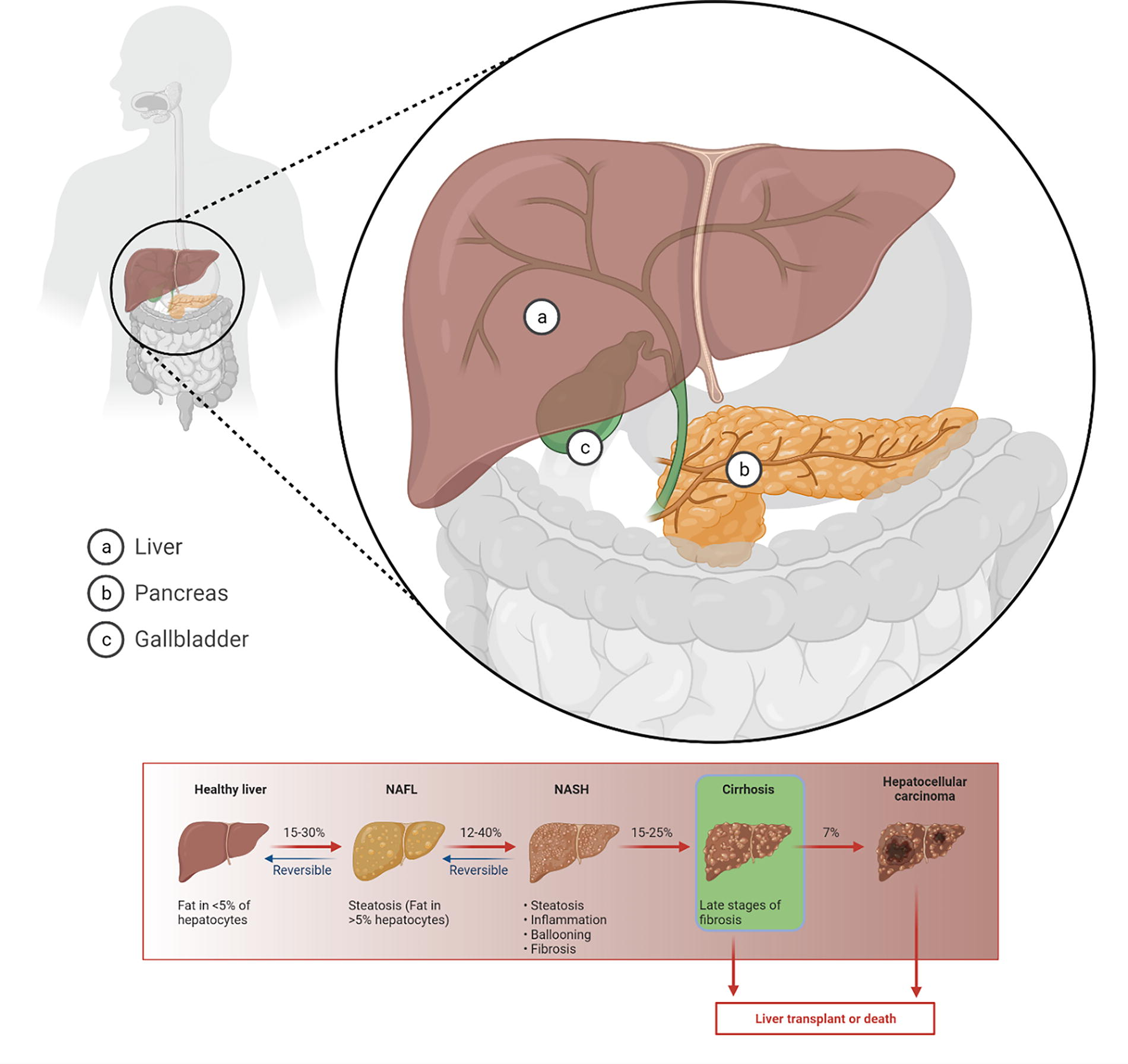
Prominent diseases of the liver.

Symptoms of liver cancer include fever, vomiting, and fatigue, prompting diagnostic steps such as blood tests, imaging scans (ultrasonography [US], magnetic resonance imaging [MRI], and computed tomography [CT]), biopsy, and laparoscopy. Despite the common use of MRI and CT for abdominal cancer imaging, researchers strive for accurate detection and classification of liver tumors through computer-aided diagnosis (CAD) systems. The CAD system involves preprocessing, attribute analysis, and classification, addressing challenges such as blurry images, environmental noises, and variations in liver size. The accurate localization and detection of lesions are crucial for structural analysis, aiding in subsequent treatments such as radiation therapy and hepatectomy.^6–9

Liver cirrhosis stands as a significant cause of morbidity and mortality in the United States, contributing to 40,000 annual deaths.¹⁰ While many patients with cirrhosis initially exhibit subclinical disease, progression can lead to rapid decompensation, elevating the risks of morbidity, mortality, and diminished quality of life.^11,12 Currently, mortality prediction relies on the Model for End Stage Sodium (MELD-Na) score, a modified logistic regression (LR) model established in 2002. While effective for short-term and high-score predictions, MELD-Na’s accuracy diminishes for lower scores and extended time frames.^13–15 With the majority of patients with cirrhosis having missing labs or low MELD-Na scores, an alternative, more comprehensive predictive method is imperative.^16,17

The inadequacy of conventional MELD-Na scores in capturing patient outcomes may stem from the intricate biological relationships among nonlinear, multidimensional variables in medicine.¹⁸ Leveraging the success of deep learning algorithms in health care applications, these models prove adept at capturing informative features, patterns, and variable interactions from complex data.¹⁹ A 2006 study demonstrated the superiority of an artificial neural network (ANN) over MELD in predicting 3-month mortality in 400 patients with end-stage liver disease.¹⁸ In a 2018 study, 500 critically ill patients with cirrhosis were examined for 12–24-hour mortality prediction using LR and long short-term memory neural networks.^20,21 Despite their contributions, these studies had limitations, including relatively small cohorts and a focus on short-term rather than long-term mortality prediction, crucial for interventions that could alter outcomes.

These contributions highlight the study’s impact on advancing liver cancer diagnostics, potentially transforming current practices and offering a more effective, accurate, and reliable tool for radiologists in the early detection and classification of liver cancer.

Related Work

Several studies^22–26 have employed machine learning models to categorize acquired images into different classes such as benign (HEM, fibrosis [FB]), CY, primary cancer (HCC, CR), and secondary cancer (MET). Table 1 provides an overview of previously developed CAD systems utilizing US, MRI, and CT modalities. Notably, studies highlighted in bold exhibit superior performance in detecting multiple disease outcomes. Diverse morphological features have been proposed for training machine learning algorithms, with deep neural network architectures consistently demonstrating the best performance. While some studies leverage texture features based on gray-level co-occurrence matrix (GLCM), others utilize convolutional neural network (CNN)-based hierarchical features instead of morphological features.^27–29

Table 1.

Detail comparison with other methods

Study	Modality	Classification	Machine learning model	Accuracy
Zhang Y et al., 2024²²	US, MRI, CT	Benign, fibrosis, cancer (primary, secondary)	DNN	Superior
Abdul Haseeb Nizamani et al., 2023²³	US, MRI, CT	Benign, fibrosis, cancer (primary, secondary)	DNN	Superior
Menegotto AB et al., 2021²⁴	US, MRI, CT	Benign, fibrosis, cancer (primary, secondary)	DNN	Superior
Jang HJ et al., 2023²⁵	US, MRI, CT	Benign, fibrosis, cancer (primary, secondary)	DNN	Superior
Naeem S et al., 2020²⁶	US, MRI, CT	Benign, fibrosis, cancer (primary, secondary)	DNN	Superior
Chaddad A et al., 2021²⁸	US	Cancer	CNN	High
Elsherbiny O et al., 2024²⁹	MRI	Cancer	CNN	High
Chiu FY et al., 2021²⁷	MRI	Cancer	CNN	High
Singh S et al., 2023³⁰	CT	Malignant liver disease (FLD vs. cirrhosis)	SVM	99.50%
Buatoom U et al., 2023³¹	MRI	CY, HEM, MA	ANN	99.70%
Chen RC et al., 2020³²	CT	Three-class voting-based classification	k-NN, SVM, RF (voting based)	N/A

ANN, artificial neural network; CNN, convolutional neural network; CT, computed tomography; DNN, deep neural network; FLD, fatty liver disease; k-NN, k-Nearest Neighbors; MRI, magnetic resonance imaging; RF, random forest; SVM, support vector machine; US, ultrasonography.

Singh presents a binary class CAD system for detecting malignant liver diseases,³⁰ specifically distinguishing between fatty liver disease and cirrhosis. The algorithm utilizes features related to coarse texture, liver size shrinkage, and nodularity. The combination of GLCM, gray-level run-length matrix, first-order statistics (FOS), Laws’, and gradient-based features is employed. The model achieves a 99.5% accuracy using support vector machine (SVM) for binary classification, although the dataset is relatively small (29 images)^31,33 demonstrating improved performance for a three-class problem (CY, HEM, and MA) using GLCM, FOS, and Laws’-based features. Principal component analysis is applied for dimensionality reduction, and ANN achieves a 99.7% accuracy for the three-class outcome. Binary classifications are performed sequentially for each class pair.

Chen proposes a voting-based classification using k-Nearest Neighbors (k-NN), SVM, and random forest models.³² Relevant feature selection based on Euclidean distance and recursive feature elimination contributes to the model’s performance in the three-class classification. These studies collectively showcase advancements in CAD systems for liver cancer diagnosis, emphasizing the effectiveness of machine learning models across different imaging modalities and disease classifications.

The discussed studies collectively form a comprehensive background in image processing, denoising, and deblurring techniques, providing valuable insights applicable to enhancing medical images for liver classification. Maier et al. introduced a 3D anisotropic hybrid diffusion technique for noise reduction in CT scans,³⁴ with principles extendable to various medical imaging modalities. Maitree et al. focused on adaptive nonlocal means denoising for MR images,³⁵ crucial for improving the quality of MR images commonly used in liver examinations. Ilesanmi et al. conducted a survey on impulse and Gaussian denoising filters,³⁶ pertinent to liver classification where image clarity is essential. Li et al. contributed to blur kernel estimation, addressing blur issues in medical images,³⁷ including those of the liver. Fundamental knowledge in digital signal processing from^38–40 is crucial for processing and analyzing medical images, a foundational understanding is essential for accurate liver classification. Buades et al. presented a review of image-denoising algorithms, including new ones, applicable in preprocessing medical images. Deep learning approaches by Yamashita et al. demonstrated the potential of CNNs in image restoration,⁴¹ a promising avenue for enhancing liver images. Iqbal et al. introduced generative adversarial nets, with applications for generating high-quality medical images,⁴² including those relevant to liver classification.

Studies by Rayyan Azam Khan et al. focused on deblurring techniques, vital for improving image clarity in medical images,⁴³ a prerequisite for accurate liver classification. Other techniques, such as those by Brattain et al.⁴⁴ and Alshagathrh et al.,⁴⁵ while not directly related to liver classification, contribute to the broader understanding of image enhancement. In summary, these studies collectively contribute to the knowledge base necessary for the related work section in the domain of liver classification, covering aspects ranging from traditional image processing techniques to advanced deep learning approaches.

The reviewed studies collectively contribute to the understanding of liver classification, combining advancements in medical image segmentation, machine learning, and CAD systems. Ansari et al.⁴⁶ conducted a survey on U-shaped networks in medical image segmentation, emphasizing their relevance in delineating liver structures for accurate classification. Alksas et al.⁴⁷ presented a machine learning-based CAD system for liver tumors, demonstrating the potential for automated diagnosis. Deep learning techniques, as explored by Zhen et al.,⁴⁸ showcased the efficacy of CNNs in identifying liver masses and HCC, contributing to the automation of classification processes. Masokano et al.⁴⁹ provided insights into the comparative assessment of texture features for cancer identification and reviewed segmentation methods in CT, both pertinent to liver classification.

Tang et al.⁵⁰ systematically reviewed CAD of liver lesions using CT images, highlighting the ongoing efforts in leveraging advanced imaging technologies for accurate classification. Chernyak et al.⁵¹ introduced the Liver Imaging Reporting and Data System (LI-RADS) system, contributing to the conceptual and historical foundation of liver classification standards. In the context of liver cancer staging, Cho et al.⁵² discussed the Barcelona Clinic Liver Cancer staging system, emphasizing its significance in predicting the survival of untreated HCC. Wu et al.⁵³ explored the applications of whole slide imaging in histopathological studies of liver disorders, providing valuable insights into the integration of digital pathology in liver classification. Studies by Wang et al.⁵⁴ delved into effective staging of fibrosis, utilizing texture features and two-photon excitation microscopy, respectively. Peng et al.⁵⁵ (Systematic Review: Diagnosis and Staging of Non-Alcoholic Fatty Liver Disease [NAFLD]/Non-Alcoholic Steatohepatitis [NASH]) conducted a systematic review on the diagnosis and staging of NAFLD and steatohepatitis, shedding light on the complexities of liver disorders.

Materials and Methods

The proposed methodology is shown in Figure 2; by using ANN, the classification is implemented.

FIG. 2.

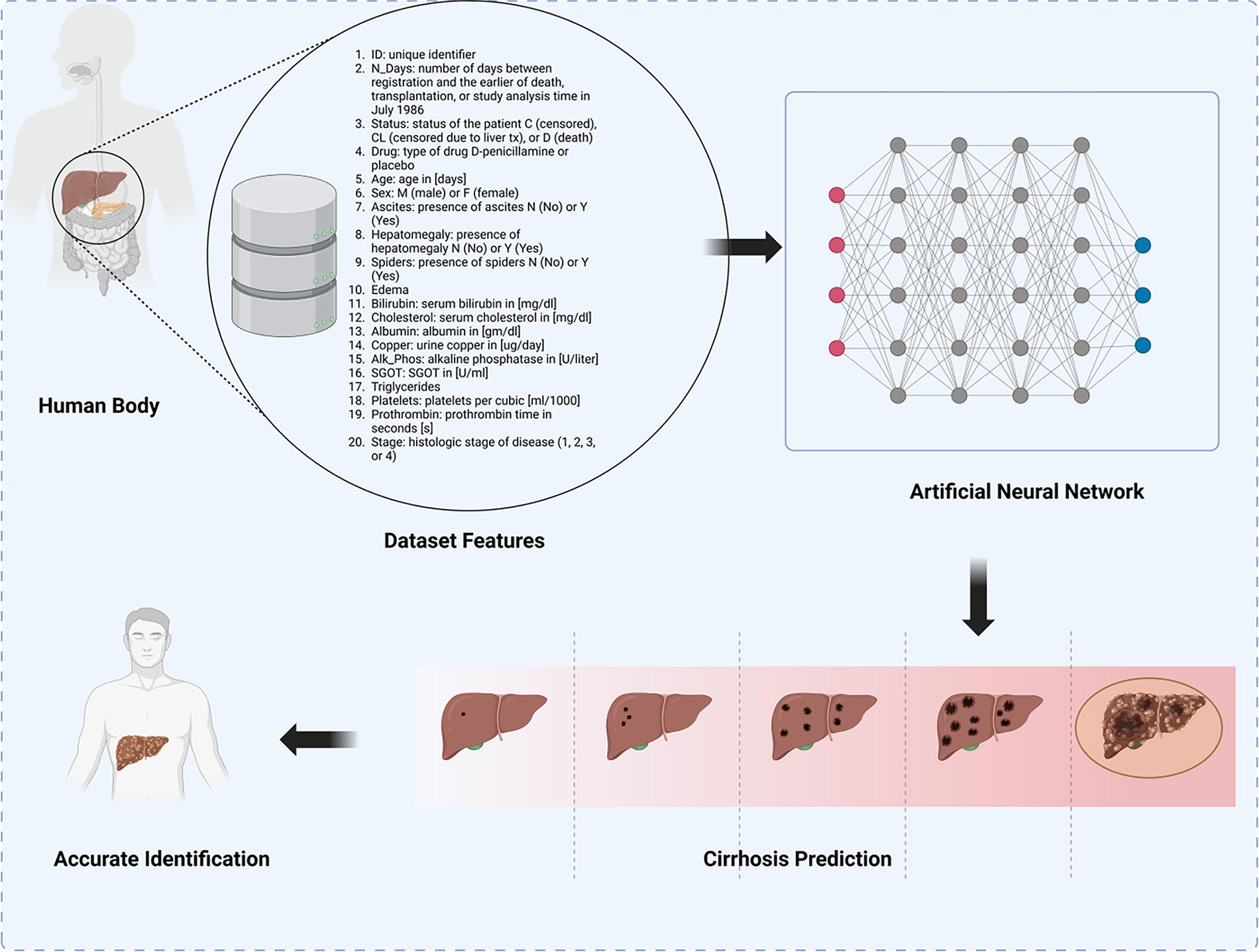
Proposed methodology block diagram.

Algorithm: Neural Network for Liver Cancer Classification Input: X: Features matrix y: Target variable (binary) test_size: Proportion of the dataset to include in the test split random_state: Seed for random number generator epochs: Number of epochs for training h batch_size: Batch size for training Output: Trained Artificial Neural Network Evaluation metrics on the test set Data Splitting: Split the dataset into training, validation, and testing sets using the train_test_split function. Preserve the class distribution in the splits. Data Standardization: Standardize the features using StandardScaler to ensure zero mean and unit variance. Model Definition: Create a Sequential model with one hidden layer containing 64 units and ReLU activation. Add an output layer with a sigmoid activation for binary classification Compile the model using the Adam optimizer and binary crossentropy loss. Model Training: Train the model on the training set, validating on the validation set Use the specified number of epochs and batch size. Plot Training History: Plot the training and validation loss over epochs Plot the training and validation accuracy over epochs Model Evaluation: Make predictions on the test set. Convert predicted probabilities to binary predictions using a threshold of 0.5 Evaluate accuracy and generate a classification report.

Dataset

The dataset originates from the Mayo Clinic trial on primary biliary cirrhosis (PBC) of the liver, conducted between 1974 and 1984. The trial aimed to assess the efficacy of the drug D-penicillamine through a randomized placebo-controlled study involving 424 patients with PBC referred to Mayo Clinic during that 10-year period. The data include the first 312 participants who participated in the randomized trial, providing comprehensive information. An additional 112 cases, while not part of the clinical trial, consented to have basic measurements recorded and be followed for survival, resulting in data on 106 additional cases. The dataset comprises various columns, including unique identifiers (ID), survival-related information (N_Days and status), drug type (D-penicillamine or placebo), demographic details (age and sex), and medical parameters (ascites, hepatomegaly, spiders, edema, bilirubin, cholesterol, albumin, copper, Alk_Phos, serum glutamic-oxaloacetic transaminase [SGOT], triglycerides, platelets, prothrombin, and stage). The feature selection is done by the provided datasets with all relevant significant features for liver disease diagnosis. Table 2 summarizes the statistical parameters for patients with liver cirrhosis.

Table 2.

Summary of statistical parameters for patients with liver cirrhosis

Statistics parameters	N_days	Age	Bilirubin	Cholesterol	Albumin	Copper	Alk_phos	SGOT	Triglycerides	Platelets	Prothrombin	Stage
Count	418	418	418	284	418	310	312	312	282	407	416	412
Mean	1917.782297	18533.35168	3.220813	369.510563	3.49744	97.648387	1982.655769	122.556346	124.702128	257.02457	10.731731	3.024272
Std	1104.672992	3815.845055	4.407506	231.944545	0.424972	85.61392	2140.388824	56.699525	65.148639	98.325585	1.022	0.882042
Min	41	9598	0.3	120	1.96	4	289	26.35	33	62	9	1
25%	1092.75	15644.5	0.8	249.5	3.2425	41.25	871.5	80.6	84.25	188.5	10	2
50%	1730	18,628	1.4	309.5	3.53	73	1259	114.7	108	251	10.6	3
75%	2613.5	21272.5	3.4	400	3.77	123	1980	151.9	151	318	11.1	4
Max	4795	28,650	28	1775	4.64	588	13862.4	457.25	598	721	18	4

SGOT, serum glutamic-oxaloacetic transaminase.

Figure 3 shows a collection of density plots, each representing the distribution of a particular variable across two different stages, denoted as “0” and “1.” These plots are commonly used in statistics to show the distribution of a dataset and to compare the distributions across different groups or conditions. The explanation of each plot is as follows:

FIG. 3.

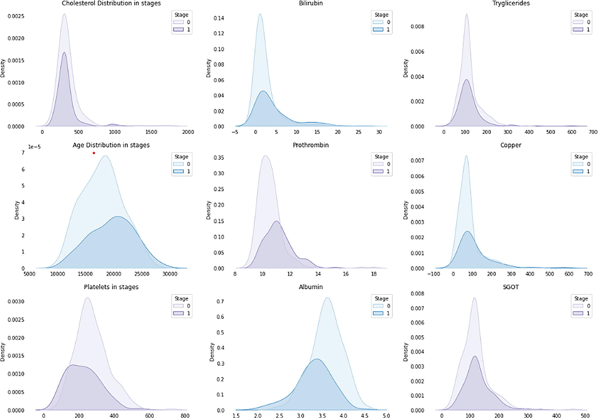
Data analysis and feature interpretation. This figure presents a series of density plots comparing the distribution of variables between two stages, labeled as “0” and “1.” Each plot shows the probability distribution of a particular variable for each stage. The x-axis represents the values of the variable, and the y-axis represents the density, indicating the concentration of data points. The shaded area under each curve represents the distribution for each stage, with the light-colored curve representing stage “0” and the dark-colored curve representing stage “1.” Overlapping sections of the curves suggest similar distributions between the two stages, whereas nonoverlapping sections highlight differences in their distributions.

Cholesterol distribution in stages: This plot shows the density distribution of cholesterol levels for two different stages. The distribution for stage 1 seems to be shifted toward higher cholesterol levels compared with stage 0.

Bilirubin: The bilirubin levels for stage 0 and stage 1 are shown here, with stage 1 again showing higher levels overall.

Triglycerides: Similar to the cholesterol plot, this shows the density distribution for triglyceride levels, with stage 1 having a distribution that indicates higher triglyceride levels.

Age distribution in stages: This shows the age distribution of subjects in two stages. Stage 0 encompasses a broader age range, whereas stage 1 seems to be concentrated in a narrower age range.

Prothrombin: This plot indicates the distribution of prothrombin levels, with stage 1 having a higher peak, suggesting higher levels of prothrombin.

Copper: The distribution of copper levels is shown, with stage 1 having a density peak at higher levels of copper.

Platelets in stages: This shows the distribution of platelet counts across two stages, with stage 1 having a distribution indicating a lower platelet count compared with stage 0.

Albumin: The density plot for albumin levels shows stage 1 with significantly lower levels than stage 0.

SGOT: This plot shows the distribution of SGOT enzyme levels in the blood, with stage 1 having higher levels.

The “stages” refer to different stages of a disease, different treatment groups, or any other categorical division within the dataset. The variables plotted are typical biochemical markers that might be measured in a clinical setting, possibly related to liver function, given the inclusion of albumin, bilirubin, and liver enzymes (SGOT). The key takeaway is that there is a noticeable difference in the distribution of these biochemical markers between the two stages, which is indicative of the progression of a disease, the effect of a treatment, or any other significant change between the two groups. This is a kind of exploratory data analysis that is used to generate hypotheses for further statistical testing.

Figure 4 contains a series of bar charts representing counts of various clinical features and treatments across two different stages of a disease, possibly a liver disease given the clinical features mentioned.

FIG. 4.

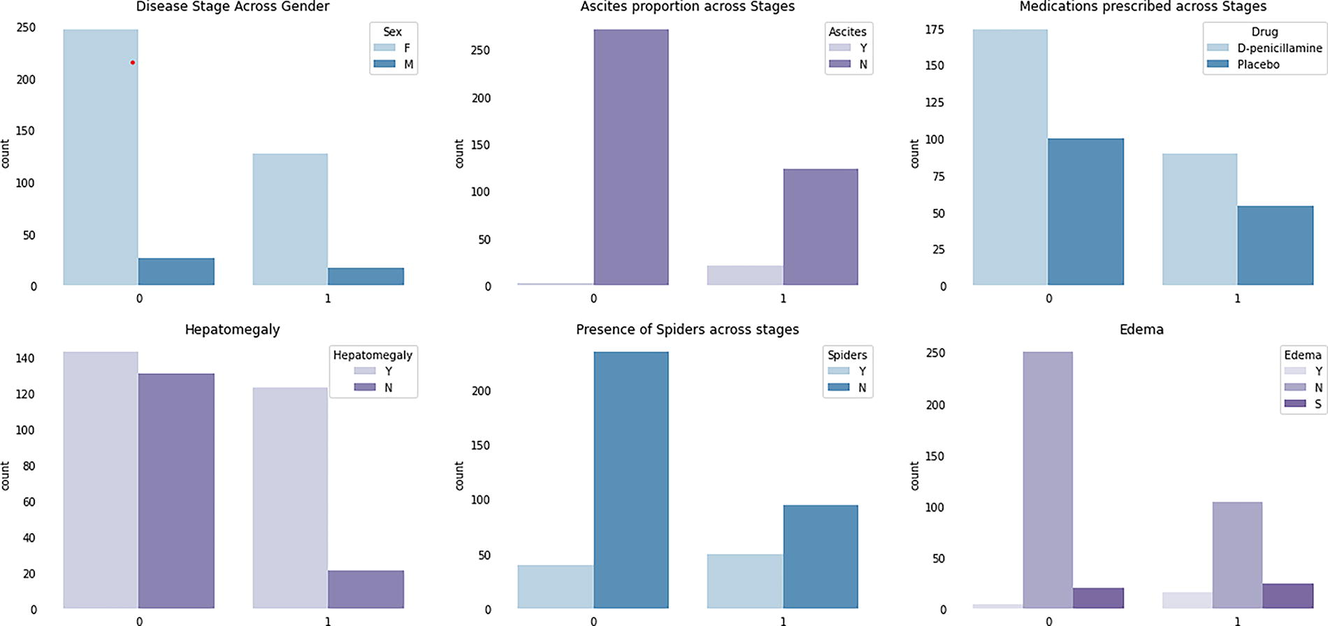
Bar chart for features of data. Each bar represents the number of occurrences or frequency of a specific feature or treatment at each disease stage. The x-axis lists the clinical features and treatments, while the y-axis shows the count of occurrences. Bars are grouped according to the two stages of the disease, allowing for a visual comparison of how clinical features and treatments vary across these stages. The lighter-colored bars represent stage “0,” and the darker-colored bars represent stage “1.”

Disease Stage Across Gender: This chart shows the count of males (M) and females (F) in two stages of the disease. Stage 0 has a higher count for both genders compared with stage 1, with more females than males in both stages.

Hepatomegaly: The chart indicates the presence (Y) or absence (N) of hepatomegaly (enlarged liver) in stages 0 and 1. In both stages, the count of patients with hepatomegaly is higher than those without, with a decrease from stage 0 to stage 1.

Ascites Proportion Across Stages: The presence (Y) or absence (N) of ascites, which is the accumulation of fluid in the peritoneal cavity, is shown for stages 0 and 1.

The bar chart demonstrates a large count of ascites presence in stage 0 and a significantly lower count in stage 1.

Presence of Spiders Across Stages: This refers to spider angiomas, a type of telangiectasias found on the skin. The count for the presence (Y) of spider angiomas is significantly higher in stage 0 than in stage 1, with the absence (N) also decreasing but to a lesser extent.

Edema: Edema, or swelling due to fluid accumulation, is categorized here as present (Y), absent (N), and possibly a third category denoted as (S), which is not standard notation and is unclear without further context. The count of edema is highest in stage 0 and drops in stage 1, with the (S) category only appearing in stage 1.

Medications Prescribed Across Stages: This chart shows the count of two different treatments prescribed across the two stages: D-penicillamine, a drug used for conditions like Wilson’s disease or rheumatoid arthritis, and a placebo. Both treatments are more commonly prescribed in stage 0 compared with stage 1, with D-penicillamine being more common than placebo.

The data suggest a progression or treatment response between stages 0 and 1, indicated by reduced counts of disease symptoms and treatments in stage 1. It may be reflective of a successful treatment protocol or natural disease progression. Without additional context, it is not possible to draw definitive conclusions.

Results and Discussion

Various evaluation matrices including training accuracy and validation accuracy, training loss and validation loss, precision, recall, F1-score, and confusion matrix are utilized to evaluate the performance of the proposed model for liver cancer classification using CT scan images. A confusion matrix helps represent the overall number of correct predictions as T_p (true positives) and the number of true labels predicted incorrectly by the model as F_n (false negatives). It also includes F_p (false positives) and T_n (true negative). It proves helpful in assessing the F1-score, accuracy, and recall of a trained model. Precision is the ratio of correctly predicted true labels to the total number of labels predicted as true by the model as follows: $Precision = \frac{T_{p}}{T_{p} + F_{p}}$ (1)

Recall, also known as sensitivity or true positive rate (TPR), is the proportion of correctly predicted true labels out of all the true labels. It is calculated by the following equation: $Recall = \frac{T_{p}}{T_{p} + F_{n}}$ (2)

The F1-score is calculated as the harmonic mean of recall and accuracy. The following criteria are used to assess model accuracy: $F 1 score = 2 x \frac{precision * recall}{p recison + recall}$ (3)

Accuracy is an evaluation metric utilized for model performance, representing the percentage of correct predictions. It indicates the total number of images correctly classified during the testing phase. It is calculated as follows: $Accuracy = \frac{T_{p} + T_{n}}{T_{p} + T_{n} + F_{p} + F_{n}}$ (4)

Table 3 appears to be a summary of classification results for a binary classifier (classes 0 and 1) using different training sample sizes (70%, 80%, and 90%). These results are often used to evaluate the performance of machine learning models. Let us break down each metric:

Table 3.

Results of the proposed model

	Precision	Recall	F1-score	Support
70% training sample
+ve case	0.79	0.93	0.85	41
No case	0.8	0.55	0.65	22
Accuracy			0.79	63
Macro avg	0.8	0.74	0.75	63
Weighted avg	0.89	0.79	0.78	63
80% training sample
+ve case	0.83	0.89	0.86	27
No case	0.77	0.67	0.71	15
Accuracy			0.81	42
Macro avg	0.83	0.78	0.79	42
Weighted avg	0.81	0.81	0.81	42
90% training sample
+ve case	0.87	0.93	0.9	14
No case	0.83	0.71	0.77	7
Accuracy			0.86	21
Macro avg	0.85	0.82	0.83	21
Weighted avg	0.86	0.86	0.85	21

As the training sample size increases (from 70% to 90%), there is a general trend of improvement in all metrics (precision, recall, F1-score, and accuracy) for both classes. This suggests that the model benefits from more training data.

For class 0 (probably the dominant class), precision, recall, and F1-score are relatively high across all training splits, indicating good model performance for this class.

For class 1, there is a notable improvement in recall and F1-score as the training sample size increases, although the precision decreases slightly in the 90% training sample. This might suggest that the model, with more data, is better at identifying true class 1 instances but also misclassifies more class 0 instances as class 1.

The accuracy of the model increases with the size of the training sample, which is a positive sign. The macro and weighted averages increase with the training sample size, suggesting an overall improvement in model performance. In summary, the model seems to perform better with a larger training sample size, particularly in identifying the less represented class (presumably class 1). However, there might be a trade-off between precision and recall for class 1 as the training size increases.

Figure 5 depicts the training and validation loss, as well as the training and validation accuracy over epochs, for a liver disease classification model trained with three different proportions of data: 70%, 80%, and 90%.

FIG. 5.

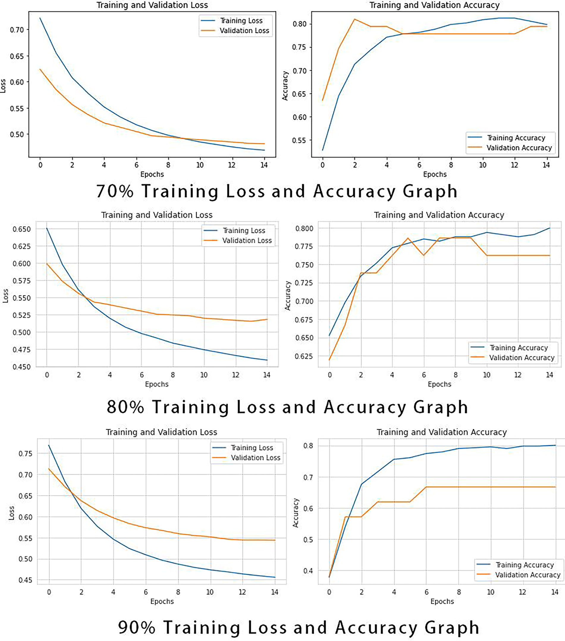
Loss and accuracy graph. This figure presents the curves depicting the training and validation loss, as well as the training and validation accuracy, over epochs for a liver disease classification model trained with different data proportions (70%, 80%, and 90%). The four curves in the figure represent the changes in training loss, validation loss, training accuracy, and validation accuracy for each data proportion. The x-axis indicates the number of epochs, while the y-axis shows the loss values and accuracy, providing a visual representation of the model’s performance with varying amounts of data.

Training and validation loss

Training Loss: It measures how well the model is fitting the training data. Ideally, this should decrease over time as the model learns.

Validation Loss: It measures how well the model performs on a separate set of data not seen during training (validation set). A decreasing trend is good, but if the validation loss increases while training loss decreases, it indicates overfitting.

Training and validation accuracy

Training Accuracy: It indicates how often the model correctly classifies the training data. This typically increases over time.

Validation Accuracy: It shows how often the model correctly classifies new data. This is critical as it provides insight into how well the model generalizes.

Analysis of graphs

70% Training Data: The validation loss decreases and then plateaus, indicating that the model might be starting to overfit as it does not improve after a certain point. The validation accuracy increases and starts to plateau, which suggests the model is achieving its best generalization on the validation set.

80% Training Data: The validation loss decreases and levels off, with a smaller gap between training and validation loss compared with the 70% training data scenario. The validation accuracy surpasses the training accuracy around the 6th epoch and continues to increase, suggesting a better generalization than the previous model. This indicates a more optimal training where the model is learning patterns that are more generalizable to unseen data.

90% Training Data: The validation loss is initially higher than the training loss but decreases sharply and starts to converge with the training loss, which is a positive sign of good model fit. However, there is a slight uptick in validation loss at the end, which suggests the beginnings of overfitting. The validation accuracy similarly improves significantly over epochs and converges toward the training accuracy, indicating the model’s improving ability to generalize.

Across all training data sizes, both training and validation losses decrease as the number of epochs increases, which is expected as the model learns from the data. The validation accuracy generally increases with more training data, suggesting that providing more data helps the model to generalize better. The difference between training and validation accuracy is smallest with 90% training data, suggesting that the model trained with more data is less prone to overfit and better at generalizing. For all three training data sizes, it appears that the models are trained sufficiently by around 10–12 epochs, as after this point, improvements in loss and accuracy are minimal.

In summary, the graphs show that the model’s performance improves with more training data and that it learns effectively over the epochs. The key is to stop training before overfitting begins, which is indicated by an increase in validation loss or a decrease in validation accuracy. The 90% training data model appears to be the most robust in terms of generalization, but care must be taken to monitor for overfitting.

Figure 6 shows the receiver operating characteristic (ROC curves and the precision–recall (PR curves for an ANN model at different levels of training data (70%, 80%, and 90%).

FIG. 6.

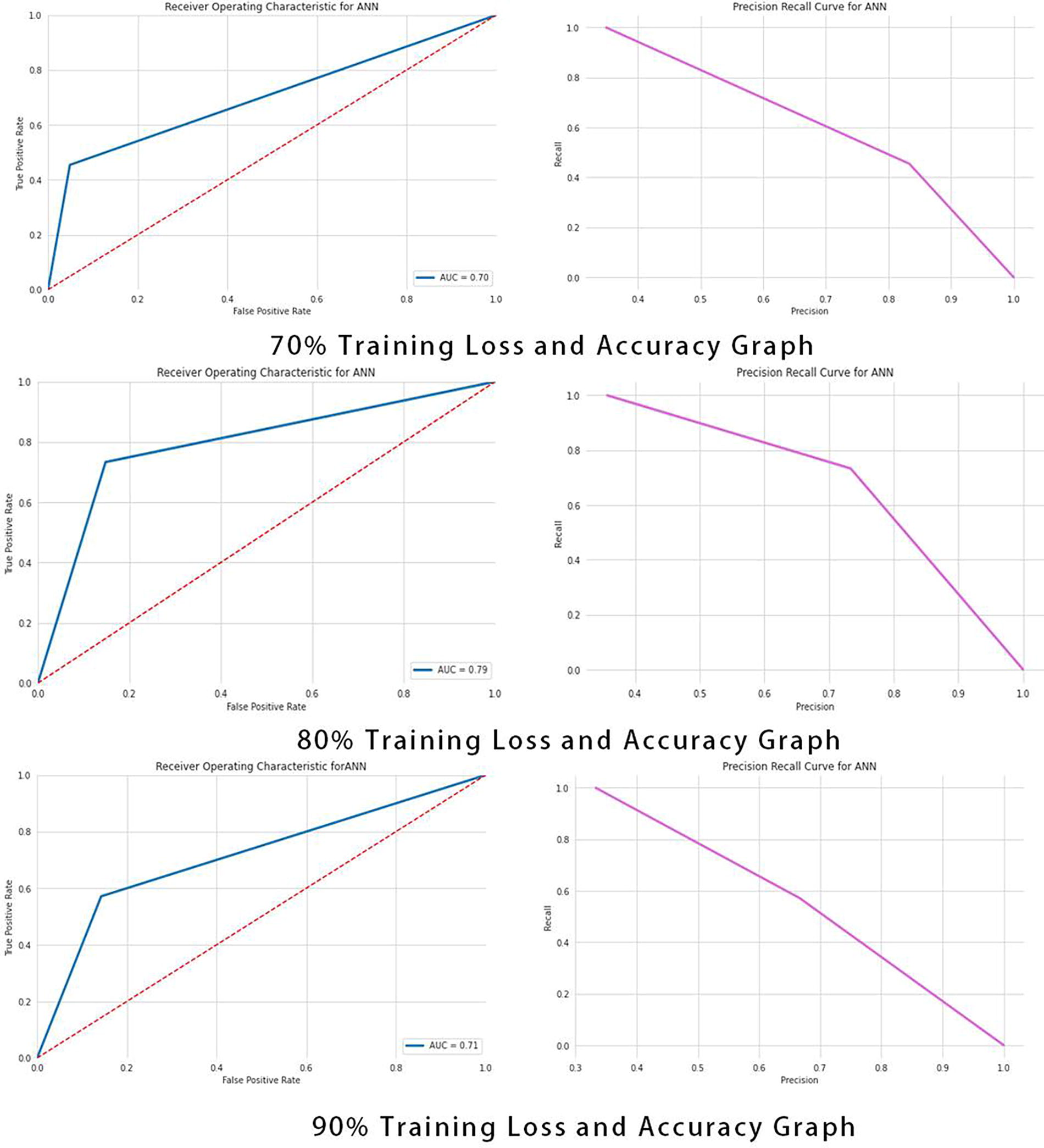
ROC graph. This figure presents the ROC curves and PR curves for an (ANN) model trained with different data proportions (70%, 80%, and 90%). The ROC curves illustrate the model’s classification performance at various thresholds, with the x-axis representing the FPR and the y-axis representing the TPR. The PR curves show the trade-off between precision and recall. ANN, artificial neural network; FPR, false positive rate; PR, precision–recall; ROC, receiver operating characteristic; TPR, true positive rate.

ROC curve

The ROC curve is a graphical plot that illustrates the diagnostic ability of a binary classifier system as its discrimination threshold is varied.

The curve is created by plotting the TPR) against the false positive rate (FPR) at various threshold settings.

Area under the curve (AUC) provides a single measure of overall performance of the classifier. An AUC of 1 indicates a perfect model, whereas an AUC of 0.5 suggests no discriminative power.

PR curve

This curve shows the trade-off between precision and recall for different threshold. A high AUC represents both high recall and high precision. Precision is a measure of result relevancy, whereas recall is a measure of how many truly relevant results are returned. The PR curve is more informative than ROC when dealing with imbalanced datasets.

Analysis

70% Training Data: The AUC for the ROC curve is 0.70, indicating moderate classification ability. The PR curve declines steeply, suggesting that precision drops quickly as recall increases, which is typical in a scenario where the positive class is less prevalent or more difficult to predict.

80% Training Data: There is an improvement in the AUC for the ROC curve to 0.79, suggesting better classification performance. The PR curve again shows a steep decline, indicating a similar trade-off between precision and recall, but the model seems to be doing better than with 70% training data.

90% Training Data: The AUC for the ROC curve is 0.71, slightly better than the 70% training data but not as high as the 80% training data. The PR curve shows that for a given recall, the precision is lower compared with the 80% training data.

The model with 80% training data seems to have the best classification performance based on the AUC of the ROC curve.

The PR curves suggest that as the recall increases, the precision of the model decreases significantly across all training data sizes.

The performance increase from 70% to 80% training data is noticeable, but there is not a significant difference in performance between the 80% and 90% training data based on these graphs alone.

The steep decline in the PR curves suggests that there may be a relatively small number of positive samples, which is common in medical datasets where the condition of interest is rare.

The model with 80% training data is showing the best performance among the three in terms of the balance between sensitivity (TPR) and specificity (FPR) as well as the balance between precision and recall. However, all models seem to struggle with maintaining precision at higher recall levels, which is a common challenge in classification tasks with imbalanced datasets.

The practical implications of this research are significant for the field of medical diagnostics. The findings highlight the potential for ANN models to play a crucial role in the early and accurate classification of liver disease. Specifically, the model trained with 80% of the available data demonstrated promising classification ability, offering health care practitioners a valuable tool for disease detection and patient risk assessment. By leveraging machine learning, health care providers may enhance the efficiency and accuracy of liver disease diagnosis, enabling timely interventions and tailored treatment plans. Moreover, these results underscore the importance of optimizing training data size and feature engineering techniques in developing robust medical diagnostic models. Ultimately, this work contributes to the ongoing effort to harness artificial intelligence (AI)-driven solutions for improved patient care and outcomes in the realm of liver disease diagnosis. This work has several limitations:

Data Size and Quality: The study may be limited by the size and quality of the dataset. Working with a larger and more diverse dataset could lead to more robust model training and evaluation.

Imbalanced Dataset: The presence of imbalanced classes in medical datasets, such as liver disease, can affect model performance. Addressing class imbalance through advanced techniques or acquiring more data for the minority class could enhance the model’s PR trade-off.

Model Complexity: The study primarily focused on ANN models. Exploring other machine learning algorithms and ensemble methods might provide alternative insights and potentially improve classification performance.

Feature Engineering: The study did not extensively investigate feature engineering techniques. Optimizing feature selection and engineering may lead to better model performance.

Generalization: While model performance was assessed rigorously, the generalization of the findings to different datasets or clinical settings should be approached with caution. Further validation on external datasets is recommended.

Interpretability: The complexity of deep learning models, such as ANNs, often leads to limited interpretability. Incorporating explainable AI techniques could enhance the model’s interpretability for clinical use.

Clinical Validation: Ultimately, the real-world clinical utility of the model should be validated through rigorous clinical trials and domain expert assessments, considering factors such as patient demographics and comorbidities.

Ethical Considerations: Ethical considerations related to privacy, informed consent, and fairness in health care AI should be thoroughly addressed when deploying such models in clinical practice.

Addressing these limitations would contribute to the development of more accurate and reliable liver disease classification models with broader applicability in medical diagnostics.

Conclusions

In conclusion, the experimental analysis of an ANN model for liver disease classification has revealed key insights into the relationship between training data volume and model performance. The comprehensive evaluation employed metrics such as precision, recall, F1-score, accuracy, and the informative curves of ROC and PR, complemented by AUC values. The model trained with 80% of the data exhibited the most effective performance, characterized by the highest AUC among the ROC curves and a favorable PR trade-off. The increase in training data from 70% to 80% significantly enhanced the model’s ability to classify liver disease more accurately. However, increasing the training data to 90% did not yield a proportional increase in performance, suggesting a potential plateau in the model’s learning capability with the given feature set and architecture. The steep decline in precision with increasing recall across all models highlights the inherent challenges in medical dataset classification tasks, particularly when dealing with imbalanced classes. These findings emphasize the importance of optimizing training data size to improve model accuracy and reliability in medical diagnostics. Future work may explore more sophisticated model architectures, feature engineering techniques, and balanced dataset approaches to mitigate the PR trade-off and enhance the model’s diagnostic precision.

Future work in this research can focus on several areas to further enhance the liver disease classification model. First, exploring advanced deep learning architectures and hyperparameter tuning may improve the model’s ability to capture complex patterns in the data. Additionally, feature engineering and selection techniques could be employed to identify the most informative features for the task. Addressing class imbalance through techniques such as oversampling or generating synthetic data points may help improve precision at higher recall levels. Finally, the model’s performance could benefit from a larger and more diverse dataset, potentially incorporating multimodal data sources such as imaging and patient history for a more comprehensive diagnostic tool.

Footnotes

Acknowledgment

The authors thank NSFC Foreign Scholars Research Fund Project：62350410483 for providing research facilities and equipment.

Authors’ Contributions

C.Z.: Contributed to the conception, design, and methodology of the study and played a central role in the coordination and oversight of the project, ensuring alignment with the study objectives. M.F.B.I.: Contributed to data collection and analysis, provided critical input during the research phase, and assisted in drafting and revising sections of the article. I.I.: Played a significant role in statistical analysis and interpretation of the data and assisted in writing key sections of the results and discussion portions of the article. M.C.: Served as the corresponding author, provided leadership in the overall management of the project, supervised the writing and finalization of the article, and facilitated communication among the team members. N.S.: Provided expertise in literature review and contributed to the theoretical framework of the study and played an active role in revising the article and ensuring it adhered to academic standards. E.M.A.: Assisted in the technical aspects of the research, including data validation and the development of computational models used in the analysis. Y.Y.G.: Contributed to the interpretation of the findings and provided critical feedback during the article preparation process and assisted in proofreading and the final revision of the document.

Author Disclosure Statement

The authors declare there is no conflict of interest.

Funding Information

This study was funded by Huanggang Normal University, China, Self-type Project of 2021 (No. 30120210103) and 2022 (No. 2042021008). This work was supported by the Princess Nourah bint Abdulrahman University Researchers Supporting Project number (PNURSP2023R384), Princess Nourah bint Abdulrahman University, Riyadh, Saudi Arabia. The authors present their appreciation to King Saud University for funding this research through Researchers Supporting Program number (RSPD2023R1006), King Saud University, Riyadh, Saudi Arabia.

Abbreviations Used

References

, Chen

, et al. Improved trends in the mortality-to-incidence ratios for liver cancer in countries with high development index and health expenditures. Healthcare (Basel), 2023; 11(2):159; doi: 10.3390/healthcare11020159

Chidambaranathan-Reghupaty

, Fisher

, Sarkar

. Hepatocellular Carcinoma (HCC): Epidemiology, etiology and molecular classification. Adv Cancer Res, 2021; 149:1–61; doi: 10.1016/bs.acr.2020.10.001

Alhatami

, Bhatti

, Huang

, et al. Review and enhancement of discrete cosine transform (DCT) for medical image fusion. In: [conference or book details], 2023; doi: 10.1007/978-981-19-9331-2_8

Ananthakrishnan

, Gogineni

, Saeian

. Epidemiology of primary and secondary liver cancers. Semin Intervent Radiol, 2006; 23(1):47–63; doi: 10.1055/s-2006-939841

Jiang

, Al-Diffhala

, Centeno

. Primary liver cancers-part 1: Histopathology, differential diagnoses, and risk stratification. Cancer Control, 2018; 25(1):1073274817744625; doi: 10.1177/1073274817744625

Hennedige

, Venkatesh

. Imaging of hepatocellular carcinoma: Diagnosis, staging and treatment monitoring. Cancer Imaging, 2013; 12(3):530–547; doi: 10.1102/1470-7330.2012.0044

Oliva

, Saini

. Liver cancer imaging: Role of CT, MRI, US and PET. Cancer Imaging, 2004; 4 Spec No A(Spec No A):S42–S46; doi: 10.1102/1470-7330.2004.0011

Yeh

, Yeung

, Apisarnthanarax

, et al. Multidisciplinary perspective of hepatocellular carcinoma: A pacific northwest experience. World J Hepatol, 2015; 7(11):1460–1483.

Gururatsakul

. Hepatology Clinical. J Gastroenterol Hepatol, 2022; 37(S1):41–102; doi: 10.1111/jgh.15951

10.

Scaglione

, Kliethermes

, Cao

, et al. The epidemiology of cirrhosis in the United States: A population-based study. J Clin Gastroenterol, 2015; 49(8):690–696; doi: 10.1097/MCG.0000000000000208

11.

Nusrat

, Khan

, Fazili

, et al. Cirrhosis and its complications: Evidence based treatment. World J Gastroenterol, 2014; 20(18):5442–5460; doi: 10.3748/wjg.v20.i18.5442

12.

Casler

, Chaney

. Cirrhosis: An evidence-based treatment approach. Nurse Pract, 2020; 45(8):16–26; doi: 10.1097/01.NPR.0000681772.39310.d0

13.

Emenena

, Emenena

, Kweki

, et al. Model for End-Stage Liver Disease (MELD) score: A tool for prognosis and prediction of mortality in patients with decompensated liver cirrhosis. Cureus, 2023; 15(5):e39267; doi: 10.7759/cureus.39267

14.

Ferrarese

, Bucci

, Zanetto

, et al. Prognostic models in end-stage liver disease. Best Pract Res Clin Gastroenterol, 2023; 67:101866; doi: 10.1016/j.bpg.2023.101866

15.

Kartoun

, Corey

, Simon

, et al. The MELD-Plus: A generalizable prediction risk score in cirrhosis. PLoS One, 2017; 12(10):e0186301.

16.

Mazumder

, Atiemo

, Daud

, et al. Patients with persistently low MELD-Na scores continue to be at risk of liver-related death. Transplantation, 2020; 104(7):1413–1418; doi: 10.1097/TP.0000000000002997

17.

Kaltenbach

, Mahmud

. Assessing the risk of surgery in patients with cirrhosis. Hepatol Commun, 2023; 7(4); doi: 10.1097/HC9.0000000000000086

18.

, Kim

, Lai

, et al. “Beyond MELD” – emerging strategies and technologies for improving mortality prediction, organ allocation and outcomes in liver transplantation. J Hepatol, 2022; 76(6):1318–1329; doi: 10.1016/j.jhep.2022.03.003

19.

Javaid

, Haleem

, Singh

, et al. Significance of machine learning in healthcare: Features, pillars and applications. Int J Intell Netw, 2022; 3:58–73; doi: 10.1016/j.ijin.2022.05.002

20.

Guo

, Mazumder

, Ladner

, et al. Predicting mortality among patients with liver cirrhosis in electronic health records with machine learning. PLoS One, 2021; 16(8):e0256428; doi: 10.1371/journal.pone.0256428

21.

Harrison

, Chang

, Hao

, et al. Using machine learning to predict near-term mortality in cirrhosis patients hospitalized at the University of Virginia health system. In: Proceedings of the 2018 Systems and Information Engineering Design Symposium (SIEDS); 2018. pp. 112–7. doi:10.1109/SIEDS.2018.8374719

22.

Zhang

, Chen

, Ma

, et al. Interactive medical image annotation using improved Attention U-net with compound geodesic distance. Expert Syst Appl, 2024; 237:121282; doi: 10.1016/j.eswa.2024.121282

23.

Nizamani

, Chen

, Nizamani

, et al. Advance brain tumor segmentation using feature fusion methods with deep U-Net model with CNN for MRI data. J King Saud Univ Comput Inf Sci, 2023; 35(9):101793; doi: 10.1016/j.jksuci.2023.101793

24.

Menegotto

, Becker

CDL

, Cazella

. Computer-aided diagnosis of hepatocellular carcinoma fusing imaging and structured health data. Health Inf Sci Syst, 2021; 9(1):20; doi: 10.1007/s13755-021-00151-x

25.

Jang

, Go

, Kim

, et al. Deep learning for the pathologic diagnosis of hepatocellular carcinoma, cholangiocarcinoma, and metastatic colorectal cancer. Cancers (Basel), 2023; 15(22):5389; doi: 10.3390/cancers15225389

26.

Naeem

, Ali

, Qadri

, et al. Machine-learning based hybrid-feature analysis for liver cancer classification using fused (MR and CT) images. Appl Sci, 2020; 10(9):3134; doi: 10.3390/app10093134

27.

Chiu

, Le

NQK

, Chen

. A multiparametric MRI-based radiomics analysis to efficiently classify tumor subregions of glioblastoma: A pilot study in machine learning. J Clin Med, 2021; 10(9):2030; doi: 10.3390/jcm10092030

28.

Chaddad

, Li

, Lu

, et al. Can autism be diagnosed with artificial intelligence? A narrative review. Diagnostics (Basel), 2021; 11(11):2032; doi: 10.3390/diagnostics11112032

29.

Elsherbiny

, Elaraby

, Alahmadi

, et al. Rapid grapevine health diagnosis based on digital imaging and deep learning. Plants (Basel), 2024; 13(1):135; doi: 10.3390/plants13010135

30.

Singh

, Hoque

, Zekry

, et al. Radiological diagnosis of chronic liver disease and hepatocellular carcinoma: A review. J Med Syst, 2023; 47(1):73; doi: 10.1007/s10916-023-01968-7

31.

Buatoom

, Jamil

. Improving classification performance with statistically weighted dimensions and dimensionality reduction. Appl Sci, 2023; 13(3):2005; doi: 10.3390/app13032005

32.

Chen

, Dewi

, Huang

, et al. Selecting critical features for data classification based on machine learning methods. J Big Data, 2020; 7(1):52; doi: 10.1186/s40537-020-00327-4

33.

Houseni

, Mahmoud

, Saad

, et al. Advanced intra-tumoural structural characterisation of hepatocellular carcinoma utilising FDG-PET/CT: A comparative study of radiomics and metabolic features in 3D and 2D. Pol J Radiol, 2021; 86:e64–e73; doi: 10.5114/pjr.2021.103239

34.

Maier

, Wigstrom

, Hofmann

, et al. Three-dimensional anisotropic adaptive filtering of projection data for noise reduction in cone beam CT. Med Phys, 2011; 38(11):5896–5909; doi: 10.1118/1.3633901

35.

Maitree

, Perez-Carrillo

GJG

, Shimony

, et al. Adaptive anatomical preservation optimal denoising for radiation therapy daily MRI. J Med Imaging (Bellingham), 2017; 4(3):34004; doi: 10.1117/1.JMI.4.3.034004

36.

Ilesanmi

, Ilesanmi

. Methods for image denoising using convolutional neural network: A review. Complex Intell Syst, 2021; 7(5):2179–2198; doi: 10.1007/s40747-021-00428-4

37.

, Wang

, Lu

, et al. Simultaneous tumor segmentation, image restoration, and blur kernel estimation in PET using multiple regularizations. Comput Vis Image Underst, 2017; 155:173–194; doi: 10.1016/j.cviu.2016.10.002

38.

Puttagunta

, Ravi

. Medical image analysis based on deep learning approach. Multimed Tools Appl, 2021; 80(16):24365–24398; doi: 10.1007/s11042-021-10707-4

39.

, Jiang

, Zhang

, et al. Medical image analysis using deep learning algorithms. Front Public Health, 2023; 11:1273253; doi: 10.3389/fpubh.2023.1273253

40.

Bhatti

, Tang

, Wu

, et al. Deep learning with graph convolutional networks: An overview and latest applications in computational intelligence. Int J Intell Syst, 2023; 2023:1–28; doi: 10.1155/2023/8342104

41.

Yamashita

, Nishio

, Do

RKG

, et al. Convolutional neural networks: An overview and application in radiology. Insights Imaging, 2018; 9(4):611–629; doi: 10.1007/s13244-018-0639-9

42.

Iqbal

, Sharif

, Yasmin

, et al. Generative adversarial networks and its applications in the biomedical image segmentation: A comprehensive survey. Int J Multimed Inf Retr, 2022; 11(3):333–368; doi: 10.1007/s13735-022-00240-x

43.

Khan

, Luo

, Wu

. Machine learning based liver disease diagnosis: A systematic review. Neurocomputing, 2022; 468:492–509; doi: 10.1016/j.neucom.2021.08.138

44.

Brattain

, Ozturk

, Telfer

, et al. Image processing pipeline for liver fibrosis classification using ultrasound shear wave elastography. Ultrasound Med Biol, 2020; 46(10):2667–2676; doi: 10.1016/j.ultrasmedbio.2020.05.016

45.

Alshagathrh

, Househ

. Artificial intelligence for detecting and quantifying fatty liver in ultrasound images: A systematic review. Bioengineering (Basel), 2022; 9(12):748; doi: 10.3390/bioengineering9120748

46.

Ansari

, Abdalla

, Ansari

, et al. Practical utility of liver segmentation methods in clinical surgeries and interventions. BMC Med Imaging, 2022; 22(1):97; doi: 10.1186/s12880-022-00825-2

47.

Alksas

, Shehata

, Saleh

, et al. A novel computer-aided diagnostic system for accurate detection and grading of liver tumors. Sci Rep, 2021; 11(1):13148; doi: 10.1038/s41598-021-91634-0

48.

Zhen

, Cheng

, Tao

, et al. Deep learning for accurate diagnosis of liver tumor based on magnetic resonance imaging and clinical data. Front Oncol, 2020; 10:680; doi: 10.3389/fonc.2020.00680

49.

Masokano

, Liu

, Xie

, et al. The application of texture quantification in hepatocellular carcinoma using CT and MRI: A review of perspectives and challenges. Cancer Imaging, 2020; 20(1):67; doi: 10.1186/s40644-020-00341-y

50.

Tang

, Duong

STM

, Nguyen

CDT

, et al. Wavelet radiomics features from multiphase CT images for screening hepatocellular carcinoma: Analysis and comparison. Sci Rep, 2023; 13(1):19559; doi: 10.1038/s41598-023-46695-8

51.

Chernyak

, Fowler

, Kamaya

, et al. Liver imaging reporting and data system (LI-RADS) version 2018: Imaging of hepatocellular carcinoma in at-risk patients. Radiology, 2018; 289(3):816–830; doi: 10.1148/radiol.2018181494i

52.

Cho

, Lee

, Song

, et al. Conditional survival estimate in patients with Barcelona Clinic Liver Cancer stage B/C hepatocellular carcinoma treated with hepatic arterial infusion chemotherapy with/without concurrent radiotherapy. Oncotarget, 2017; 8(45):79914–79926; doi: 10.18632/oncotarget.20321

53.

, Moeckel

. Application of digital pathology and machine learning in the liver, kidney and liver diseases. J Pathol Inform, 2023; 14:100184; doi: 10.1016/j.jpi.2022.100184

54.

Wang

, Wang

, Gao

, et al. Evaluation of texture features at staging liver fibrosis based on phase contrast X-ray imaging. Biomed Eng Online, 2018; 17(1):179; doi: 10.1186/s12938-018-0612-3

55.

Peng

, Stewart

, Woodman

, et al. Non-alcoholic steatohepatitis: A review of its mechanism, models and medical treatments. Front Pharmacol, 2020; 11:603926; doi: 10.3389/fphar.2020.603926