A Model to Predict the Permeation Kinetics of Dimethyl Sulfoxide in Articular Cartilage

Abstract

Cryopreservation of articular cartilage (AC) has excited great interest due to the practical surgical importance of this tissue. Characterization of permeation kinetics of cryoprotective agents (CPA) in AC is important for designing optimal CPA addition/removal protocols to achieve successful cryopreservation. Permeation is predominantly a mass diffusion process. Since the diffusivity is a function of temperature and concentration, analysis of the permeation problem would be greatly facilitated if a predictive method were available. This article describes, a model that was developed to predict the permeation kinetics of dimethyl sulfoxide (DMSO) in AC. The cartilage was assumed as a porous medium, and the effect(s) of composition and thermodynamic nonideality of the DMSO solution were considered in model development. The diffusion coefficient was correlated to the infinite dilution coefficients through a binary diffusion thermodynamic model. The UNIFAC model was used to evaluate the activity coefficient, the Vignes equation was employed to estimate the composition dependence of the diffusion coefficient, and the Siddiqi-Lucas correlation was applied to determine the diffusion coefficients at infinite dilution. Comparisons of the predicted overall DMSO uptake by AC with the experimental data over wide temperature and concentration ranges [1∼37°C, 10∼47% (w/w)] show that the model can accurately describe the permeation kinetics of DMSO in AC [coefficient of determination (R²): 0.961∼0.996, mean relative error (MRE): 2.2∼9.1%].

Introduction

The cryopreservation of articular cartilage (AC) has excited great interest due to the practical surgical importance of this tissue.^1,2 Vitrification has been considered as the most promising method to cryopreserve AC by maintaining the viability of chondrocytes, as well as the integrity of extracelluar matrix.^3–5 The current approach to vitrification requires introduction of high concentrations of cryoprotective agents (CPA). Sufficient permeation throughout the tissue and minimization of accompanying damage to the cells, such as osmotic stress and cellular toxicity, are required for a successful vitrification protocol. The low chondrocyte viability observed by Brockbank et al. after implementing so-called vitreous preservation to porcine AC⁶ could be related to the fact that only the cells near the surface were protected by a sufficient concentration of CPA. Jomha et al.'s investigation of the effects of increasing dimethyl sulfoxide (DMSO) concentrations on chondrocyte recovery in intact porcine AC⁷ demonstrated that high DMSO concentration confers significant protection from cryoinjury, but is compromised by significant osmotic stress and cellular toxicity. Therefore, in order to achieve successful vitrification, a reasonable design of CPA addition/removal protocols is very important. A proper mathematical model to describe the CPA permeation kinetics in AC will help to fulfill such task.

Permeation is dominantly a mass diffusion process. Fick's second law of diffusion was often used for permeation modeling, wherein the diffusion coefficient was regarded as a constant—the apparent diffusion coefficient—and determined by fitting to the experimental measurements of average DMSO concentration in AC samples.^8–10 Recently, Zhang and Pegg¹¹ utilized a triphasic model originating from biomechanical engineering principles to describe water and CPA transport in AC, and Abazari et al.^12,13 did further work to make it more accurate. The triphasic description of the permeation of CPA is more robust, taking into account the nonideality of the CPA solution and the deformation of the tissue. However, experimental overall CPA uptake data are also needed to obtain the best fit value of the diffusion coefficient, which is considered as a constant despite the concentration. In addition, the entire triphasic model is quite complex, involving multiple coupled partial differential equations (PDE), and is not accessed easily.

Since the diffusivity is a function of temperature and concentration, the analysis of the permeation problem would be greatly facilitated if a predictive method were available. In this study, a relatively simple model that considers the effect(s) of concentration and thermodynamic nonideality on the diffusion coefficient was developed. The model has the ability to predict the permeation kinetics of DMSO in AC. Experiments over wide temperature and concentration ranges were carried out to validate the proposed model.

Model development

Model assumptions

The following assumptions were incorporated in development of the model.

1. No DMSO is generated or consumed in AC, no DMSO is transported by convection, and there are no temperature and pressure gradients.

2. Tissue size and density remain constant during permeation.

3. Tissue has porous structure. This is a good assumption for AC, which is described as a network of pores and tortuosity.¹⁴

4. DMSO diffusion is spatially isotropic in AC. Although the cartilage is not homogeneous, this assumption is justified because of its high water content (∼80%),¹⁵ and the low molecular weight and nonelectrolyte nature of DMSO.

5. The composition dependence and nonideal behavior of DMSO diffusion in AC are similar to those in bulk solution. The relatively small molecular size of DMSO (van der Waals radius: ∼0.26 nm, calculated from atomic increments¹⁶) in comparison with the water–filled diffusion channels in cartilage (average radius: 2∼4 nm¹⁴) makes this assumption reasonable.

6. We neglected DMSO uptake by the chondrocytes. This is a reasonable assumption since the chondrocytes comprise only about 1%–2% of tissue volume.¹⁵

7. The solution is binary, consisting of DMSO and water (i.e., ignoring the effect of other trace components, such as NaCl).

Governing equations

Based on the assumptions above, the diffusion of DMSO in AC can be described by the equation of continuity below in mass units.¹⁷ \documentclass{aastex}\usepackage{amsbsy}\usepackage{amsfonts}\usepackage{amssymb}\usepackage{bm}\usepackage{mathrsfs}\usepackage{pifont}\usepackage{stmaryrd}\usepackage{textcomp}\usepackage{portland,xspace}\usepackage{amsmath,amsxtra}\pagestyle{empty}\DeclareMathSizes{10}{9}{7}{6} \begin{document} \begin{align*} \frac {\partial \omega_ {\rm d}} {\partial t} = \nabla \cdot (D_ {\rm d , AC} ^ {\rm eff} \nabla\omega_ {\rm d}) . \tag {\rm {Eq.} \ 1} \end{align*} \end{document}

The effective diffusion coefficient, \documentclass{aastex}\usepackage{amsbsy}\usepackage{amsfonts}\usepackage{amssymb}\usepackage{bm}\usepackage{mathrsfs}\usepackage{pifont}\usepackage{stmaryrd}\usepackage{textcomp}\usepackage{portland, xspace}\usepackage{amsmath, amsxtra}\pagestyle{empty}\DeclareMathSizes {10} {9} {7} {6} \begin{document} $$D_{\rm d , AC}^{\rm eff}$$ \end{document} , was determined by the equation derived by Maroudas,¹⁴ using a tortuosity factor and the diffusion coefficient of a substance in water: \documentclass{aastex}\usepackage{amsbsy}\usepackage{amsfonts}\usepackage{amssymb}\usepackage{bm}\usepackage{mathrsfs}\usepackage{pifont}\usepackage{stmaryrd}\usepackage{textcomp}\usepackage{portland,xspace}\usepackage{amsmath,amsxtra}\pagestyle{empty}\DeclareMathSizes{10}{9}{7}{6} \begin{document} \begin{align*} D_ {\rm d , AC} ^ {\rm eff} = D_ {\rm dw} \frac {H} { \lambda^2} . \tag {\rm {Eq.} \ 2} \end{align*} \end{document}

The diffusion coefficient of DMSO in water, \documentclass{aastex}\usepackage{amsbsy}\usepackage{amsfonts}\usepackage{amssymb}\usepackage{bm}\usepackage{mathrsfs}\usepackage{pifont}\usepackage{stmaryrd}\usepackage{textcomp}\usepackage{portland, xspace}\usepackage{amsmath, amsxtra}\pagestyle{empty}\DeclareMathSizes {10} {9} {7} {6} \begin{document} $$D_{\rm dw}$$ \end{document} , can be reasonably represented by an equation with the form¹⁸ \documentclass{aastex}\usepackage{amsbsy}\usepackage{amsfonts}\usepackage{amssymb}\usepackage{bm}\usepackage{mathrsfs}\usepackage{pifont}\usepackage{stmaryrd}\usepackage{textcomp}\usepackage{portland,xspace}\usepackage{amsmath,amsxtra}\pagestyle{empty}\DeclareMathSizes{10}{9}{7}{6} \begin{document} \begin{align*} D_{\rm dw} = D_0 \Gamma^m. \tag{\rm{Eq.} \ 3} \end{align*} \end{document}

The thermodynamic factor, \documentclass{aastex}\usepackage{amsbsy}\usepackage{amsfonts}\usepackage{amssymb}\usepackage{bm}\usepackage{mathrsfs}\usepackage{pifont}\usepackage{stmaryrd}\usepackage{textcomp}\usepackage{portland, xspace}\usepackage{amsmath, amsxtra}\pagestyle{empty}\DeclareMathSizes {10} {9} {7} {6} \begin{document} $$\Gamma$$ \end{document} , portraying the nonideal behavior, can be expressed by \documentclass{aastex}\usepackage{amsbsy}\usepackage{amsfonts}\usepackage{amssymb}\usepackage{bm}\usepackage{mathrsfs}\usepackage{pifont}\usepackage{stmaryrd}\usepackage{textcomp}\usepackage{portland,xspace}\usepackage{amsmath,amsxtra}\pagestyle{empty}\DeclareMathSizes{10}{9}{7}{6} \begin{document} \begin{align*} \Gamma = 1 + x_{\rm d} \left(\frac {\partial {\rm ln} \gamma_{\rm d}} {\partial x_{\rm d}} \right). \tag {\rm {Eq.} \ 4} \end{align*} \end{document}

The activity coefficient for DMSO, \documentclass{aastex}\usepackage{amsbsy}\usepackage{amsfonts}\usepackage{amssymb}\usepackage{bm}\usepackage{mathrsfs}\usepackage{pifont}\usepackage{stmaryrd}\usepackage{textcomp}\usepackage{portland, xspace}\usepackage{amsmath, amsxtra}\pagestyle{empty}\DeclareMathSizes {10} {9} {7} {6} \begin{document} $$\gamma_{\rm d}$$ \end{document} , was estimated using the UNIFAC model.^19,20 The reference diffusion coefficient, \documentclass{aastex}\usepackage{amsbsy}\usepackage{amsfonts}\usepackage{amssymb}\usepackage{bm}\usepackage{mathrsfs}\usepackage{pifont}\usepackage{stmaryrd}\usepackage{textcomp}\usepackage{portland, xspace}\usepackage{amsmath, amsxtra}\pagestyle{empty}\DeclareMathSizes {10} {9} {7} {6} \begin{document} $$D_0$$ \end{document} , is a function of the diffusion coefficients at infinite dilution and the composition of the mixture. The Vignes equation^18,21 was used to estimate it: \documentclass{aastex}\usepackage{amsbsy}\usepackage{amsfonts}\usepackage{amssymb}\usepackage{bm}\usepackage{mathrsfs}\usepackage{pifont}\usepackage{stmaryrd}\usepackage{textcomp}\usepackage{portland,xspace}\usepackage{amsmath,amsxtra}\pagestyle{empty}\DeclareMathSizes{10}{9}{7}{6} \begin{document} \begin{align*} D_0 = (D_{\rm dw}^0) ^{x_{\rm w}} (D_{\rm wd}^0) ^{x_{\rm d}}. \tag{\rm{Eq.} \ 5} \end{align*} \end{document}

The Siddiqi-Lucas correlation²² was chosen to determine \documentclass{aastex}\usepackage{amsbsy}\usepackage{amsfonts}\usepackage{amssymb}\usepackage{bm}\usepackage{mathrsfs}\usepackage{pifont}\usepackage{stmaryrd}\usepackage{textcomp}\usepackage{portland, xspace}\usepackage{amsmath, amsxtra}\pagestyle{empty}\DeclareMathSizes {10} {9} {7} {6} \begin{document} $$D_{\rm dw}^0$$ \end{document} and \documentclass{aastex}\usepackage{amsbsy}\usepackage{amsfonts}\usepackage{amssymb}\usepackage{bm}\usepackage{mathrsfs}\usepackage{pifont}\usepackage{stmaryrd}\usepackage{textcomp}\usepackage{portland, xspace}\usepackage{amsmath, amsxtra}\pagestyle{empty}\DeclareMathSizes {10} {9} {7} {6} \begin{document} $$D_{\rm wd}^0$$ \end{document} , expressed respectively as: \documentclass{aastex}\usepackage{amsbsy}\usepackage{amsfonts}\usepackage{amssymb}\usepackage{bm}\usepackage{mathrsfs}\usepackage{pifont}\usepackage{stmaryrd}\usepackage{textcomp}\usepackage{portland,xspace}\usepackage{amsmath,amsxtra}\pagestyle{empty}\DeclareMathSizes{10}{9}{7}{6} \begin{document} \begin{align*} D_{\rm dw}^0 = (2.98 \times 10^{- 7}) \eta_{\rm w}^{- 1.026}V_{\rm b , d}^{- 0.5473}T , \tag{\rm{Eq.} \ 6} \end{align*} \end{document} \documentclass{aastex}\usepackage{amsbsy}\usepackage{amsfonts}\usepackage{amssymb}\usepackage{bm}\usepackage{mathrsfs}\usepackage{pifont}\usepackage{stmaryrd}\usepackage{textcomp}\usepackage{portland,xspace}\usepackage{amsmath,amsxtra}\pagestyle{empty}\DeclareMathSizes{10}{9}{7}{6} \begin{document} \begin{align*} D_{\rm wd}^0 = 9.89 \times 10^{- 8} \eta_{\rm d}^{- 0.907}V_{\rm b , d}^{- 0.45}V_{\rm b , w}^{0.265}T. \tag{\rm{Eq.} \ 7} \end{align*} \end{document}

The viscosity of DMSO, \documentclass{aastex}\usepackage{amsbsy}\usepackage{amsfonts}\usepackage{amssymb}\usepackage{bm}\usepackage{mathrsfs}\usepackage{pifont}\usepackage{stmaryrd}\usepackage{textcomp}\usepackage{portland, xspace}\usepackage{amsmath, amsxtra}\pagestyle{empty}\DeclareMathSizes {10} {9} {7} {6} \begin{document} $$\eta_{\rm d}$$ \end{document} , was determined by the Vogel-Fulcher-Tammann-Hesse (VFTH) equation:^23,24 \documentclass{aastex}\usepackage{amsbsy}\usepackage{amsfonts}\usepackage{amssymb}\usepackage{bm}\usepackage{mathrsfs}\usepackage{pifont}\usepackage{stmaryrd}\usepackage{textcomp}\usepackage{portland,xspace}\usepackage{amsmath,amsxtra}\pagestyle{empty}\DeclareMathSizes{10}{9}{7}{6} \begin{document} \begin{align*} {\rm ln} \eta_ {\rm d} = {A} + \frac {B} {{T} - {T} _0} , \tag {\rm {Eq.} \ 8} \end{align*} \end{document}

and the viscosity of water, \documentclass{aastex}\usepackage{amsbsy}\usepackage{amsfonts}\usepackage{amssymb}\usepackage{bm}\usepackage{mathrsfs}\usepackage{pifont}\usepackage{stmaryrd}\usepackage{textcomp}\usepackage{portland, xspace}\usepackage{amsmath, amsxtra}\pagestyle{empty}\DeclareMathSizes {10} {9} {7} {6} \begin{document} $$\eta_{\rm w}$$ \end{document} , was calculated using the free volume model:²⁵ \documentclass{aastex}\usepackage{amsbsy}\usepackage{amsfonts}\usepackage{amssymb}\usepackage{bm}\usepackage{mathrsfs}\usepackage{pifont}\usepackage{stmaryrd}\usepackage{textcomp}\usepackage{portland,xspace}\usepackage{amsmath,amsxtra}\pagestyle{empty}\DeclareMathSizes{10}{9}{7}{6} \begin{document} \begin{align*} \eta_ {\rm w} = \eta_0 \ {\rm exp} \left[ \frac {V_ {\rm w} ^ {*}} {(K / \beta) (K^ {\prime} - T_ {\rm g , w} + T )} \right] . \tag {\rm {Eq.} \ 9} \end{align*} \end{document}

The molar volumes at the normal boiling point of DMSO \documentclass{aastex}\usepackage{amsbsy}\usepackage{amsfonts}\usepackage{amssymb}\usepackage{bm}\usepackage{mathrsfs}\usepackage{pifont}\usepackage{stmaryrd}\usepackage{textcomp}\usepackage{portland, xspace}\usepackage{amsmath, amsxtra}\pagestyle{empty}\DeclareMathSizes {10} {9} {7} {6} \begin{document} $$(V_{\rm b,d})$$ \end{document} and water \documentclass{aastex}\usepackage{amsbsy}\usepackage{amsfonts}\usepackage{amssymb}\usepackage{bm}\usepackage{mathrsfs}\usepackage{pifont}\usepackage{stmaryrd}\usepackage{textcomp}\usepackage{portland, xspace}\usepackage{amsmath, amsxtra}\pagestyle{empty}\DeclareMathSizes {10} {9} {7} {6} \begin{document} $$(V_{\rm b,w})$$ \end{document} were estimated by the Tyn-Calus equation,²⁰ respectively, that is, \documentclass{aastex}\usepackage{amsbsy}\usepackage{amsfonts}\usepackage{amssymb}\usepackage{bm}\usepackage{mathrsfs}\usepackage{pifont}\usepackage{stmaryrd}\usepackage{textcomp}\usepackage{portland,xspace}\usepackage{amsmath,amsxtra}\pagestyle{empty}\DeclareMathSizes{10}{9}{7}{6} \begin{document} \begin{align*} V_{\rm b} = 0.285V_{\rm c}^{1.048}. \tag{\rm{Eq.} \ 10} \end{align*} \end{document}

Initial and boundary conditions

There is no DMSO initially present inside \documentclass{aastex}\usepackage{amsbsy}\usepackage{amsfonts}\usepackage{amssymb}\usepackage{bm}\usepackage{mathrsfs}\usepackage{pifont}\usepackage{stmaryrd}\usepackage{textcomp}\usepackage{portland, xspace}\usepackage{amsmath, amsxtra}\pagestyle{empty}\DeclareMathSizes {10} {9} {7} {6} \begin{document} $${\rm AC} \ [ i.e. , \omega_{\rm d} (t = 0) = 0 ].$$ \end{document} The first kind of boundary condition (i.e., constant DMSO concentration on the AC surfaces), was used and assumed to equal the equilibrium concentration of DMSO \documentclass{aastex}\usepackage{amsbsy}\usepackage{amsfonts}\usepackage{amssymb}\usepackage{bm}\usepackage{mathrsfs}\usepackage{pifont}\usepackage{stmaryrd}\usepackage{textcomp}\usepackage{portland, xspace}\usepackage{amsmath, amsxtra}\pagestyle{empty}\DeclareMathSizes {10} {9} {7} {6} \begin{document} $$(\omega_{\rm e})$$ \end{document} inside the tissue achieved during the permeation process (see below for the determination of \documentclass{aastex}\usepackage{amsbsy}\usepackage{amsfonts}\usepackage{amssymb}\usepackage{bm}\usepackage{mathrsfs}\usepackage{pifont}\usepackage{stmaryrd}\usepackage{textcomp}\usepackage{portland, xspace}\usepackage{amsmath, amsxtra}\pagestyle{empty}\DeclareMathSizes {10} {9} {7} {6} \begin{document} $$\omega_{\rm e}$$ \end{document} ).

Materials and Methods

Measurement of DMSO permeation into AC

Permeation experiments over wide temperature and concentration ranges, as listed in Table 1, were carried out to validate the developed model.

Table 1.

Permeation Experiment Conditions

Temperature (°C)	Exposure concentration [%(w/w)]	Exposure time (min)
1	10	0, 1, 2, 5, 10, 20, 30, and 60
	19	0, 5, 10, 20, 30, and 60
	28	0, 5, 10, 20, 30, and 60
	38	0, 2, 5, 10, 30, 60, and 120
	47	0, 2, 5, 10, 30, 60, and 120
22	10	0, 1, 2, 5, 10, 20, 30, and 60
37	10	0, 1, 2, 5, 10, 20, 30, and 60

The chemicals used in the experiments, unless otherwise specified, were all purchased from Sinopharm Chemical Reagent Co. Ltd., Shanghai, China, and were of analytical grade. Distilled water was used throughout the experiments. To avoid phosphate precipitation, the DMSO solutions were prepared with a HEPES-buffered medium (145 mmol/L Na⁺, 3.3 mmol/L K⁺, and 20 mmol/L HEPES) instead of phosphate-buffered saline (PBS).²⁶ The HEPES was obtained from Amresco, USA.

AC samples were harvested from the back knee joints of approximately 12-month-old lambs that were killed for food in a local commercial abattoir. AC discs without bone (6 mm diameter, ∼0.8 mm thickness) were taken from the weight-bearing portion using a corneal trephine and a scalpel, and stored in ice-cold HEPES-buffered medium for later use.

The experimental procedures are similar to that we previously described,²⁷ briefly as follows. Each AC disc was blotted, and weighed (W1), and immersed in 2 mL DMSO solution for its stated exposure time. After exposure, each disc was removed, blotted, quickly rinsed in distilled water, reblotted, and weighed again (W2), and then placed in sealed vials containing 2 mL distilled water to allow the DMSO to migrate out. The DMSO was quantified by ultraviolet (UV) spectrophotometry.²⁷ Six replications were undertaken for each exposure time. The DMSO concentration in each AC disc was expressed in weight terms: \documentclass{aastex}\usepackage{amsbsy}\usepackage{amsfonts}\usepackage{amssymb}\usepackage{bm}\usepackage{mathrsfs}\usepackage{pifont}\usepackage{stmaryrd}\usepackage{textcomp}\usepackage{portland,xspace}\usepackage{amsmath,amsxtra}\pagestyle{empty}\DeclareMathSizes{10}{9}{7}{6} \begin{document} \begin{align*} {\rm DMSO} [\% ({\rm w} / {\rm w})] = \frac {W_ {\rm D} } {W 2 - W 1 \times (1 - m_ {\rm w})} \times 100 , \tag { \rm {Eq.} \ 11} \end{align*} \end{document}

Determination of the equilibrium concentration

The equilibrium concentration \documentclass{aastex}\usepackage{amsbsy}\usepackage{amsfonts}\usepackage{amssymb}\usepackage{bm}\usepackage{mathrsfs}\usepackage{pifont}\usepackage{stmaryrd}\usepackage{textcomp}\usepackage{portland, xspace}\usepackage{amsmath, amsxtra}\pagestyle{empty}\DeclareMathSizes {10} {9} {7} {6} \begin{document} $$(\omega_{\rm e})$$ \end{document} , for a specific permeation, is determined to be the mean value of all the measured data after permeation achieving equilibrium, calculated as \documentclass{aastex}\usepackage{amsbsy}\usepackage{amsfonts}\usepackage{amssymb}\usepackage{bm}\usepackage{mathrsfs}\usepackage{pifont}\usepackage{stmaryrd}\usepackage{textcomp}\usepackage{portland,xspace}\usepackage{amsmath,amsxtra}\pagestyle{empty}\DeclareMathSizes{10}{9}{7}{6} \begin{document} \begin{align*} \omega_ { \rm e } = \frac { \sum { \bar { \omega } } _ { { \rm d } , i }} {{ \rm N } + 1 - { n } _ { \rm e } } \quad ( i = n_ { \rm e } , n_ { \rm e } + 1 , \ldots \ldots , N ) , \tag { \rm { Eq. } \ 12 } \end{align*} \end{document}

where N is the total number of exposure time points (as Table 1, column 3 shows), \documentclass{aastex}\usepackage{amsbsy}\usepackage{amsfonts}\usepackage{amssymb}\usepackage{bm}\usepackage{mathrsfs}\usepackage{pifont}\usepackage{stmaryrd}\usepackage{textcomp}\usepackage{portland, xspace}\usepackage{amsmath, amsxtra}\pagestyle{empty}\DeclareMathSizes {10} {9} {7} {6} \begin{document} $${\bar {\omega}}_{\rm d}$$ \end{document} is the average DMSO concentration in AC measured at certain time point, and \documentclass{aastex}\usepackage{amsbsy}\usepackage{amsfonts}\usepackage{amssymb}\usepackage{bm}\usepackage{mathrsfs}\usepackage{pifont}\usepackage{stmaryrd}\usepackage{textcomp}\usepackage{portland, xspace}\usepackage{amsmath, amsxtra}\pagestyle{empty}\DeclareMathSizes {10} {9} {7} {6} \begin{document} $$n_{\rm e}$$ \end{document} is the number of the time point that exposures reached equilibrium (adjudged by t-test with a significance level of 0.05).

Numerical method

The geometry of the AC disc is considered as a perfect cylinder, and DMSO can penetrate into the disc from the peripheral side as well as the top and bottom surfaces. A finite element method (FEM) was applied, and the model was solved with COMSOL Multiphysics^®. All parameter values needed in the model calculation are listed in Table 2.

Table 2.

Parameter Values Adopted in Model Calculation

DMSO	A	B	T₀ (K)	V_c,d (ml/mol)
	−1.9528^a	331.80^a	172.41^a	228^b

Water	η₀ (mPa·s)	V_w^* (ml/g)	K/β [ml/(g·K)]	K’ (K)	T_g,w (K)	V_c,w (ml/mol)
	3.33×10⁻² ^c	0.91^c	1.945×10⁻³ ^c	−19.73^c	136^c	56^b

Others	H	λ	m
	0.777^d	1.4^e	0.5^f

Determined by fitting Eq. (8) to the data reported in Ref. 29; ^bFrom Ref. 30; ^cFrom Ref. 25; ^dFrom Ref. 28; ^eFrom Ref. 14; ^fFrom Ref. 31.

Evaluation of model prediction accuracy

The coefficient of determination \documentclass{aastex}\usepackage{amsbsy}\usepackage{amsfonts}\usepackage{amssymb}\usepackage{bm}\usepackage{mathrsfs}\usepackage{pifont}\usepackage{stmaryrd}\usepackage{textcomp}\usepackage{portland, xspace}\usepackage{amsmath, amsxtra}\pagestyle{empty}\DeclareMathSizes {10} {9} {7} {6} \begin{document} $$(R^2)$$ \end{document} and mean relative error (MRE) were adopted to evaluate the accuracy of model prediction. \documentclass{aastex}\usepackage{amsbsy}\usepackage{amsfonts}\usepackage{amssymb}\usepackage{bm}\usepackage{mathrsfs}\usepackage{pifont}\usepackage{stmaryrd}\usepackage{textcomp}\usepackage{portland, xspace}\usepackage{amsmath, amsxtra}\pagestyle{empty}\DeclareMathSizes {10} {9} {7} {6} \begin{document} $$R^2$$ \end{document} and MRE were defined as follows, respectively. \documentclass{aastex}\usepackage{amsbsy}\usepackage{amsfonts}\usepackage{amssymb}\usepackage{bm}\usepackage{mathrsfs}\usepackage{pifont}\usepackage{stmaryrd}\usepackage{textcomp}\usepackage{portland,xspace}\usepackage{amsmath,amsxtra}\pagestyle{empty}\DeclareMathSizes{10}{9}{7}{6} \begin{document} \begin{align*} R^2 = \frac {\left[\mathop \sum \limits_ {i = 1} ^N x_i y_i - \mathop\sum \limits_ {i = 1} ^N x_i \mathop\sum \limits_ {i = 1} ^N y_i \bigg / N \right] ^2} {\left[\mathop \sum \limits_ {i = 1} ^N x_i^2 - \left(\mathop \sum \limits_ {i = 1} ^N x_i \right) ^2 \Bigg / N \right] \left[\mathop \sum \limits_ {i = 1} ^N y_i^2 - \left(\mathop \sum \limits_ {i = 1} ^N y_i \right) ^2 \Bigg/ N \right]} , \tag {\rm {Eq.} \ 13} \end{align*} \end{document} \documentclass{aastex}\usepackage{amsbsy}\usepackage{amsfonts}\usepackage{amssymb}\usepackage{bm}\usepackage{mathrsfs}\usepackage{pifont}\usepackage{stmaryrd}\usepackage{textcomp}\usepackage{portland,xspace}\usepackage{amsmath,amsxtra}\pagestyle{empty}\DeclareMathSizes{10}{9}{7}{6} \begin{document} \begin{align*} {\rm MRE} \ (\%) = \frac {1} {N} \mathop\sum \limits_ {i = 1} ^N \left| \frac {y_i - x_i} {x_i} \times 100 \right| , \tag {\rm {Eq.} \ 14} \end{align*} \end{document}

where x and y denote experimental and predicted values of average DMSO concentration in the AC disc, respectively.

Results and Discussion

The experimental results of overall DMSO uptake by AC discs are shown in Figure 1 for different exposure concentrations and temperatures, together with the model predictions. The resulting values of \documentclass{aastex}\usepackage{amsbsy}\usepackage{amsfonts}\usepackage{amssymb}\usepackage{bm}\usepackage{mathrsfs}\usepackage{pifont}\usepackage{stmaryrd}\usepackage{textcomp}\usepackage{portland, xspace}\usepackage{amsmath, amsxtra}\pagestyle{empty}\DeclareMathSizes {10} {9} {7} {6} \begin{document} $$R^2$$ \end{document} and MRE range from 0.961 to 0.996 and 2.2% to 9.1%, specifically, 0.963 and 9.1% for case [1°C, 10%(w/w)], 0.961 and 7.2% for [22°C, 10%(w/w)], 0.985 and 3.9% for [37°C, 10%(w/w)], 0.986 and 3.9% for [1°C, 19%(w/w)], 0.995 and 2.2% for [1°C, 28%(w/w)], 0.996 and 3.6% for [1°C, 38%(w/w)], and 0.994 and 3.7% for [1°C, 47%(w/w)], where the contents inside the square brackets represent the case conditions. High values of \documentclass{aastex}\usepackage{amsbsy}\usepackage{amsfonts}\usepackage{amssymb}\usepackage{bm}\usepackage{mathrsfs}\usepackage{pifont}\usepackage{stmaryrd}\usepackage{textcomp}\usepackage{portland, xspace}\usepackage{amsmath, amsxtra}\pagestyle{empty}\DeclareMathSizes {10} {9} {7} {6} \begin{document} $$R^2$$ \end{document} indicate that the simulated results agree very well with the experimental data for all cases. The values for MRE do not look as perfect as those of \documentclass{aastex}\usepackage{amsbsy}\usepackage{amsfonts}\usepackage{amssymb}\usepackage{bm}\usepackage{mathrsfs}\usepackage{pifont}\usepackage{stmaryrd}\usepackage{textcomp}\usepackage{portland, xspace}\usepackage{amsmath, amsxtra}\pagestyle{empty}\DeclareMathSizes {10} {9} {7} {6} \begin{document} $$R^2$$ \end{document} , especially for cases [1°C, 10%(w/w)] and [22°C, 10%(w/w)]. Major contributions to the MRE value are from the initial stage of permeation, which we ascribe to experimental error due to the initial rapid permeation rate.

FIG. 1.

Time course of overall DMSO uptakes by AC disc at different exposure temperatures [(a) 1°C, (b) 22°C, and (c) 37°C] and concentrations [(d), Concentrations of the exposure solutions indicated beside the corresponding lines and symbols]. Symbols, experimental values; Solid lines: model predictions. Error bars represent the standard deviations (SD).

Under all the conditions tested, the equilibrium DMSO concentration in AC discs \documentclass{aastex}\usepackage{amsbsy}\usepackage{amsfonts}\usepackage{amssymb}\usepackage{bm}\usepackage{mathrsfs}\usepackage{pifont}\usepackage{stmaryrd}\usepackage{textcomp}\usepackage{portland, xspace}\usepackage{amsmath, amsxtra}\pagestyle{empty}\DeclareMathSizes {10} {9} {7} {6} \begin{document} $$(\omega_{\rm e})$$ \end{document} stabilized at about 90% of the concentration of the surrounding exposure solution. This is consistent with the results of other researchers^9,28 and our previous study,²⁷ which might be due to the existence of an equilibrium pressure difference between the cartilage and its surrounding solution, and the existence of “bound” water (i.e., nonsolvent water) in the tissue (detailed discussions can be found in Refs. 11 and 32). In light of such a concentration imbalance between the AC disc and its surrounding solution, it is reasonable, for simulation, to treat the boundary concentration as 90% of that of the exposure solution directly, when no experimental data are available. The time needed to achieve permeation equilibrium decreases with increasing temperature as expected (about 20, 10, and 5 min for 1, 22, and 37°C, respectively). Apparently, this time seems not affected by the concentration of exposure solution. This can be attributed to the effects of both concentration gradient and diffusion coefficient-composition relationship: (1). A higher concentration of exposure solution means a larger concentration gradient between the cartilage matrix and the surrounding solution (i.e., larger driving force for diffusion); (2). Equation 5 represents that \documentclass{aastex}\usepackage{amsbsy}\usepackage{amsfonts}\usepackage{amssymb}\usepackage{bm}\usepackage{mathrsfs}\usepackage{pifont}\usepackage{stmaryrd}\usepackage{textcomp}\usepackage{portland, xspace}\usepackage{amsmath, amsxtra}\pagestyle{empty}\DeclareMathSizes {10} {9} {7} {6} \begin{document} $$D_0$$ \end{document} varies with the mole fraction of one of the components between the two extreme values, \documentclass{aastex}\usepackage{amsbsy}\usepackage{amsfonts}\usepackage{amssymb}\usepackage{bm}\usepackage{mathrsfs}\usepackage{pifont}\usepackage{stmaryrd}\usepackage{textcomp}\usepackage{portland, xspace}\usepackage{amsmath, amsxtra}\pagestyle{empty}\DeclareMathSizes {10} {9} {7} {6} \begin{document} $$D_{\rm dw}^0$$ \end{document} and \documentclass{aastex}\usepackage{amsbsy}\usepackage{amsfonts}\usepackage{amssymb}\usepackage{bm}\usepackage{mathrsfs}\usepackage{pifont}\usepackage{stmaryrd}\usepackage{textcomp}\usepackage{portland, xspace}\usepackage{amsmath, amsxtra}\pagestyle{empty}\DeclareMathSizes {10} {9} {7} {6} \begin{document} $$D_{\rm wd}^0$$ \end{document} , which implies that the diffusion coefficient of DMSO in water, \documentclass{aastex}\usepackage{amsbsy}\usepackage{amsfonts}\usepackage{amssymb}\usepackage{bm}\usepackage{mathrsfs}\usepackage{pifont}\usepackage{stmaryrd}\usepackage{textcomp}\usepackage{portland, xspace}\usepackage{amsmath, amsxtra}\pagestyle{empty}\DeclareMathSizes {10} {9} {7} {6} \begin{document} $$D_{\rm dw}$$ \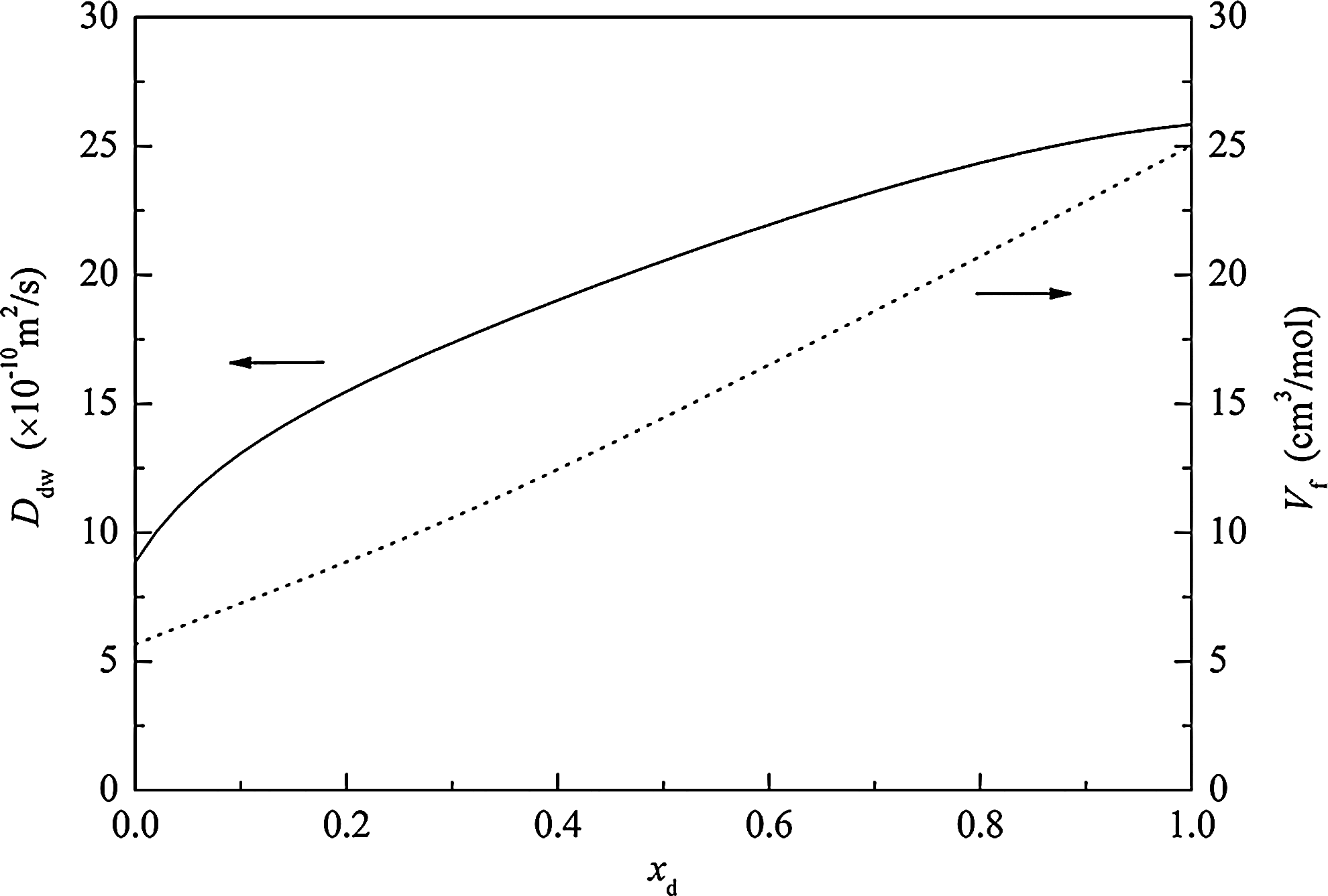end{document} , also varies between its two limiting values, according to Equations 3 and 5. As illustrated in Figure 2, \documentclass{aastex}\usepackage{amsbsy}\usepackage{amsfonts}\usepackage{amssymb}\usepackage{bm}\usepackage{mathrsfs}\usepackage{pifont}\usepackage{stmaryrd}\usepackage{textcomp}\usepackage{portland, xspace}\usepackage{amsmath, amsxtra}\pagestyle{empty}\DeclareMathSizes {10} {9} {7} {6} \begin{document} $$D_{\rm dw}$$ \end{document} increases with increasing DMSO mole fraction. Such a diffusion coefficient–composition relationship could be explained qualitatively using the free volume theory which is based on the idea that molecular transport occurs by the translation of molecules from one free space to another defined by the potential cage of their neighbors.^33,34 The larger the free volume, the more possible for a molecule to jump into its neighboring void (i.e., the faster the diffusion). The molar free volume of the binary DMSO-water solution, \documentclass{aastex}\usepackage{amsbsy}\usepackage{amsfonts}\usepackage{amssymb}\usepackage{bm}\usepackage{mathrsfs}\usepackage{pifont}\usepackage{stmaryrd}\usepackage{textcomp}\usepackage{portland, xspace}\usepackage{amsmath, amsxtra}\pagestyle{empty}\DeclareMathSizes {10} {9} {7} {6} \begin{document} $$V_{\rm f}$$ \end{document} , can be calculated as¹⁶ \documentclass{aastex}\usepackage{amsbsy}\usepackage{amsfonts}\usepackage{amssymb}\usepackage{bm}\usepackage{mathrsfs}\usepackage{pifont}\usepackage{stmaryrd}\usepackage{textcomp}\usepackage{portland,xspace}\usepackage{amsmath,amsxtra}\pagestyle{empty}\DeclareMathSizes{10}{9}{7}{6} \begin{document} \begin{align*} V_ {\rm f} = \frac {x_ {\rm d} M_ {\rm d} + x_ {\rm w} M_ {\rm w}} {\rho} - (\nu_ {\rm vdw , d} + \nu_ {\rm vdw , w}) N_ {\rm A} , \tag {\rm {Eq.} \ 15} \end{align*} \end{document}

where \documentclass{aastex}\usepackage{amsbsy}\usepackage{amsfonts}\usepackage{amssymb}\usepackage{bm}\usepackage{mathrsfs}\usepackage{pifont}\usepackage{stmaryrd}\usepackage{textcomp}\usepackage{portland, xspace}\usepackage{amsmath, amsxtra}\pagestyle{empty}\DeclareMathSizes {10} {9} {7} {6} \begin{document} $$\nu_{\rm vdw , d}$$ \end{document} and \documentclass{aastex}\usepackage{amsbsy}\usepackage{amsfonts}\usepackage{amssymb}\usepackage{bm}\usepackage{mathrsfs}\usepackage{pifont}\usepackage{stmaryrd}\usepackage{textcomp}\usepackage{portland, xspace}\usepackage{amsmath, amsxtra}\pagestyle{empty}\DeclareMathSizes {10} {9} {7} {6} \begin{document} $$\nu_{\rm vdw , w}$$ \end{document} are the van der Waals volumes of DMSO and water, \documentclass{aastex}\usepackage{amsbsy}\usepackage{amsfonts}\usepackage{amssymb}\usepackage{bm}\usepackage{mathrsfs}\usepackage{pifont}\usepackage{stmaryrd}\usepackage{textcomp}\usepackage{portland, xspace}\usepackage{amsmath, amsxtra}\pagestyle{empty}\DeclareMathSizes {10} {9} {7} {6} \begin{document} $$M_{\rm d}$$ \end{document} and \documentclass{aastex}\usepackage{amsbsy}\usepackage{amsfonts}\usepackage{amssymb}\usepackage{bm}\usepackage{mathrsfs}\usepackage{pifont}\usepackage{stmaryrd}\usepackage{textcomp}\usepackage{portland, xspace}\usepackage{amsmath, amsxtra}\pagestyle{empty}\DeclareMathSizes {10} {9} {7} {6} \begin{document} $$M_{\rm w}$$ \end{document} are the molecular weights of DMSO and water, respectively, \documentclass{aastex}\usepackage{amsbsy}\usepackage{amsfonts}\usepackage{amssymb}\usepackage{bm}\usepackage{mathrsfs}\usepackage{pifont}\usepackage{stmaryrd}\usepackage{textcomp}\usepackage{portland, xspace}\usepackage{amsmath, amsxtra}\pagestyle{empty}\DeclareMathSizes {10} {9} {7} {6} \begin{document} $$\rho$$ \end{document} is the solution density, and \documentclass{aastex}\usepackage{amsbsy}\usepackage{amsfonts}\usepackage{amssymb}\usepackage{bm}\usepackage{mathrsfs}\usepackage{pifont}\usepackage{stmaryrd}\usepackage{textcomp}\usepackage{portland, xspace}\usepackage{amsmath, amsxtra}\pagestyle{empty}\DeclareMathSizes {10} {9} {7} {6} \begin{document} $$N_{\rm A}$$ \end{document} is Avogadro's number. The van der Waals volume can be calculated from atomic increments,¹⁶ and for the solution density available data are reported in the literature.³⁵ It can be seen from Figure 2 that the molar free volume of the DMSO–water solution increases with increasing DMSO mole fraction, basically consistent with that of \documentclass{aastex}\usepackage{amsbsy}\usepackage{amsfonts}\usepackage{amssymb}\usepackage{bm}\usepackage{mathrsfs}\usepackage{pifont}\usepackage{stmaryrd}\usepackage{textcomp}\usepackage{portland, xspace}\usepackage{amsmath, amsxtra}\pagestyle{empty}\DeclareMathSizes {10} {9} {7} {6} \begin{document} $$D_{\rm dw}$$ \end{document} vs. \documentclass{aastex}\usepackage{amsbsy}\usepackage{amsfonts}\usepackage{amssymb}\usepackage{bm}\usepackage{mathrsfs}\usepackage{pifont}\usepackage{stmaryrd}\usepackage{textcomp}\usepackage{portland, xspace}\usepackage{amsmath, amsxtra}\pagestyle{empty}\DeclareMathSizes {10} {9} {7} {6} \begin{document} $$x_{\rm d}$$ \end{document} .

FIG. 2.

Diffusion coefficient of DMSO in water and molar free volume of aqueous DMSO solution as a function of concentration (25°C).

Apart from the overall uptake of CPA by tissue, the spatial CPA concentration change history is also very important. During the loading process, although the CPA concentration at the surface layer of the AC increases quickly, it takes a longer time for full permeation of CPA into the deeper layers depending on the sample size.⁸ This gives rise to the nonuniformity of CPA concentration over the whole tissue, which means that chondrocytes at different positions are exposed to different CPA concentrations for different times, leading to different osmotic and toxicity responses of the cells. Accurate quantification of the spatial and temporal mass transport process of CPA in the cartilage is a critical requirement for addressing issues of osmotic volume excursions and CPA-induced cytotoxicity. Here, a comparison was made between the transient spatial DMSO concentration distributions produced, respectively, by the presently developed model (named Model-I) and the commonly used traditional Fick's second law of diffusion (named Model-II). The diffusion coefficients for Model-II were obtained by least squares fit implemented in COMSOL Multiphysics^®, and they were listed in Table 3 together with the values of \documentclass{aastex}\usepackage{amsbsy}\usepackage{amsfonts}\usepackage{amssymb}\usepackage{bm}\usepackage{mathrsfs}\usepackage{pifont}\usepackage{stmaryrd}\usepackage{textcomp}\usepackage{portland, xspace}\usepackage{amsmath, amsxtra}\pagestyle{empty}\DeclareMathSizes {10} {9} {7} {6} \begin{document} $$R^2$$ \end{document} and MRE. The comparative R² and MRE values of Model-I and Model-II validate the accuracy of the presently developed model from another side. The simulated results reveal that the two models give different spatial DMSO concentration change histories, as illustrated in Figure 3 for case [1°C, 19%(w/w)]. However, experimental measurements would be essential to investigate the actual spatial and temporal CPA distribution in the tissue. Magnetic resonance imaging (MRI) is an often-adopted method to do such measurements.^36–39 The recent work by Bernemann et al.⁴⁰ demonstrates that computer tomography (CT) can also be an effective technique.

FIG. 3.

Predicted concentration profiles of DMSO in AC disc by Model-I (solid lines) and Model-II (dashed lines), respectively, as a function of exposure time. The abscissa represents the axial line of the AC disc with Point 1 at 0 mm and Point 2 at the furthest point to the right. Exposure temperature: 1°C, exposure concentration: 19%(w/w).

Table 3.

Diffusion Coefficients for Model-II

T (°C)	1					22	37
C [%(w/w)]	10	19	28	38	47	10	10
D (×10⁻¹⁰m²/s)	2.59 (2.46)	1.60	1.90	1.68	1.65	4.40 (4.06)	6.75
R ²	0.97	0.99	1.00	1.00	1.00	0.96	1.00
MRE (%)	8.7	4.4	2.5	0.7	1.7	6.6	1.8

C, exposure concentration; D, diffusion coefficient of DMSO in AC; T, exposure temperature. The blanketed values are from Ref. 11.

Finally, one should note that although the proposed model was validated only for DMSO in the present study, it could be extended to other CPA species, such as glycerol and propanediol, due to the universal characteristics of the governing equations. Corresponding parameter values for Equation 8 should be obtained and more proper correlations might be chosen to replace Equations 5 –7 for a specific CPA. The viscosity of a pure substance is easily searchable in the literature. For the equations to calculate diffusion coefficient in infinite dilution, one can refer to Ref. 18 which gives a complete summary. In any case, experimental verification is obviously essential.

Conclusions

A model to predict the permeation kinetics of DMSO in articular cartilage was developed that takes into account the effects of concentration and thermodynamic nonideality of the solution. The model was validated by excellent congruence of the model predictions and the experimental measurements over wide temperature and concentration ranges. With such a model, spatial and temporal DMSO distribution in AC could be predicted directly. The model developed in this study could help researchers understand the concentration change behavior of CPA in tissues, and thereby optimize the process of CPA addition/removal.

Footnotes

Author Disclosure Statement

This research was supported by the Fundamental Research Funds for Central Universities (No. 2012QNA4008). No competing financial interests exist.

References

Jomha

. Approaches to the cryopreservation of articular cartilage. PhD Thesis. University of Alberta, 2003.

Pegg

, Wusteman

, Wang

. Cryopreservation of articular cartilage. Part 1: Conventional cryopreservation methods. Cryobiology, 2006; 52:335–346.

Pegg

, Wang

, Vaughan

. Cryopreservation of articular cartilage. Part 3: The liquidus-tracking method. Cryobiology, 2006; 52:360–368.

Song

, Lightfoot

, Chen

et al. Vitreous preservation of rabbit articular cartilage. Cell Preserv Technol, 2004; 2:67–74.

Onari

, Hayashi

, Ozaki

et al. Vitreous preservation of articular cartilage from cryoinjury in rabbits. Cryobiology, 2012; 65:98–103.

Brockbank

KGM

, Chen

, Song

. Vitrification of porcine articular cartilage. Cryobiology, 2010; 60:217–221.

Jomha

, Anoop

, Bagnall

et al. Effects of increasing concentrations of dimethyl sulfoxide during cryopreservation of porcine articular cartilage. Cell Preserv Technol, 2002; 1:111–120.

Muldrew

, Sykes

, Schachar

et al. Permeation kinetics of dimethyl sulfoxide in articular cartilage. CryoLetters, 1996; 17:331–340.

Sharma

, Law

, Rehieh

et al. A novel method to measure cryoprotectant permeation into intact articular cartilage. Cryobiology, 2007; 54:196–203.

10.

Jomha

, Law

, Abazari

et al. Permeation of several cryoprotectant agents into porcine articular cartilage. Cryobiology, 2009; 58:110–114.

11.

Zhang

, Pegg

. Analysis of the permeation of cryoprotectants in cartilage. Cryobiology, 2007; 54:146–153.

12.

Abazari

, Elliott

JAW

, Law

et al. A biomechanical triphasic approach to the transport of nondilute solutions in articular cartilage. Biophys J, 2009; 97:3054–3064.

13.

Abazari

, Thompson

, Elliott

JAW

et al. Transport phenomena in articular cartilage cryopreservation as predicted by the modified triphasic model and the effect of natural inhomogeneities. Biophys J, 2012; 102:1284–1293.

14.

Maroudas

. Physicochemical properties of articular cartilage. Adult Articular Cartilage. Freeman

MAR

. unbridge Wells, England: Pitman Medical, 1979; 131–170Cited by Muldrew K, Sykes B, Schachar N, et al. Permeation kinetics of dimethyl sulfoxide in articular cartilage. CryoLetters 1996;17:331–340.

15.

Wei

. Articular Cartilage. Beijing: Science Press, 2007(in Chinese).

16.

Edward

. Molecular volumes and the Stokes-Einstein equation. J Chem Edu, 1970; 47:261–270.

17.

Bird

, Stewart

, Lightfoot

. Transport Phenomena, 2nd. New York: John Wiley & Sons, Inc., 2002.

18.

Taylor

, Krishna

. Multicomponent Mass Transfer. New York: John Wiley & Sons, Inc., 1993.

19.

Fredenslund

, Jones

, Prausnitz

. Group-contribution estimation of activity coefficients in nonideal liquid mixtures. AIChE J, 1975; 21:1086–1099.

20.

Dong

, Fang

, Chen

. Principles of Properties Estimation and Computer Calculations. Beijing: Chemical Industry Press, 2006(in Chinese).

21.

Vignes

. Diffusion in binary solutions. Variation of diffusion coefficient with composition. Ind Eng Chem Fundamen, 1966; 5:189–199.

22.

Siddiqi

, Lucas

. Correlations for prediction of diffusion in liquids. Can J Chem Eng, 1986; 64:839–843.

23.

Viswanath

, Ghosh

, Prasad

et al. Viscosity of Liquids. Theory, Estimation, Experiment, and Data. The Netherlands: Springer, 2007.

24.

Nascimento

MLF

, Aparicio

. Data classification with the Vogel–Fulcher–Tammann–Hesse viscosity equation using correspondence analysis. Physica B, 2007; 398:71–77.

25.

, Fowler

, Toner

. Water activity and mobility in solutions of glycerol and small molecular weight sugars. J Appl Phys, 2006; 100:074702.

26.

Wusteman

, Pegg

, Robinson

et al. Vitrification media: Toxicity, permeability, and dielectric properties. Cryobiology, 2002; 44:24–37.

27.

Zhang

, Yu

, Chen

. Permeation of dimethyl sulfoxide into articular cartilage at subzero temperatures. J Zhejiang Univ.-Sci. B (Biomed Biotechnol), 2012; 13:213–220.

28.

Pegg

, Wang

, Vaughan

. Cryopreservation of articular cartilage. Part 2: Mechanisms of cryoinjury. Cryobiology, 2006; 52:347–359.

29.

Springer Materials. http://www.springermaterials.com/docs/info/978-3-540-75486-2_53.html. 2013 January 23.

30.

CRC Handbook of Chemistry and Physics, 92ndInternet Version 2012.

31.

Kosanovich

, Cullinan

Jr . A study of molecular transport in liquid mixtures based on the concept of ultimate volume. Ind Eng Chem Fundamen, 1976; 15:41–45.

32.

Elmoazzen

, Elliott

JAW

, McGann

. Cryoprotectant equilibration in tissues. Cryobiology, 2005; 51:85–91.

33.

Turnbull

, Cohen

. Free-volume model of the amorphous phase: Glass transition. J Chem Phys, 1961; 34:120–125.

34.

Cohen

, Turnbull

. Molecular transport in liquids and glasses. J Chem Phys, 1959; 31:1164–1169.

35.

Grande

, Juliá

, García

et al. On the density and viscosity of (water+ dimethylsulphoxide) binary mixtures. J Chem Thermodynam, 2007; 39:1049–1056.

36.

Isbell

, Fyfe

, Ammons

RLM

et al. Measurement of cryoprotective solvent penetration into intact organ tissues using high-field NMR microimaging. Cryobiology, 1997; 35:165–172.

37.

Abazari

, Elliott

JAW

, McGann

et al. MR spectroscopy measurement of the diffusion of dimethyl sulfoxide in articular cartilage and comparison to theoretical predictions. Osteoarthr Cartilage, 2012; 20:1004–1010.

38.

Carsi

, Lopez-Lacomba

, Sanz

et al. Cryoprotectant permeation through human articular cartilage. Osteoarthr Cartilage, 2004; 12:787–792.

39.

Han

, Ma

, Benson

et al. Measurement of the apparent diffusivity of ethylene glycol in mouse ovaries through rapid MRI and theoretical investigation of cryoprotectant perfusion procedures. Cryobiology, 2009; 58:298–302.

40.

Bernemann

, Manuchehrabadi

, Spindler

et al. Diffusion of dimethyl sulfoxide in tissue engineered collagen scaffolds visualized by computer tomography. CryoLetters, 2010; 31:493–503.