Comparative Study on Two Different Methods for Determination of Hydraulic Conductivity of HeLa Cells During Freezing

Abstract

Background:

The measurement of hydraulic conductivity of the cell membrane is very important for optimizing the protocol of cryopreservation and cryosurgery. There are two different methods using differential scanning calorimetry (DSC) to measure the freezing response of cells and tissues. Devireddy et al. presented the slow-fast-slow (SFS) cooling method, in which the difference of the heat release during the freezing process between the osmotically active and inactive cells is used to obtain the cell membrane hydraulic conductivity and activation energy. Luo et al. simplified the procedure and introduced the single-slow (SS) cooling protocol, which requires only one cooling process although different cytocrits are required for the determination of the membrane transport properties. To the best of our knowledge, there is still a lack of comparison of experimental processes and requirements for experimental conditions between these two methods. This study made a systematic comparison between these two methods from the aforementioned aspects in detail.

Methods:

The SFS and SS cooling methods mentioned earlier were utilized to obtain the reference hydraulic conductivity (L_pg) and activation energy (E_Lp) of HeLa cells by fitting the model to DSC data.

Results:

With the SFS method, it was determined that L_pg = 0.10 μm/(min·atm) and E_Lp = 22.9 kcal/mol; whereas the results obtained by the SS cooling method showed that L_pg = 0.10 μm/(min·atm) and E_Lp = 23.6 kcal/mol.

Conclusions:

The results indicated that the values of the water transport parameters measured by two methods were comparable. In other words, the two parameters can be obtained by comparing the heat releases between two slow cooling processes of the same sample according to the SFS method. However, the SS method required analyzing heat releases of samples with different cytocrits. Thus, more experimental time was required.

Introduction

Cryopreservation of cells, tissues, and organs is an enabling technology for modern cell-based medicine. Cryopreservation mainly consists of three steps: freezing, storage, and thawing. Both the freezing and thawing processes are crucial to determine the viability of cells.^1,2 Therefore, a quantitative understanding of the freezing response of cells via measuring the hydraulic conductivity of the cell membrane at subzero temperatures is crucial to the design of an optimal freezing and thawing protocol to maximize cell survival post-cryopreservation.^2–4

Cryomicroscopy has been the most commonly used technique for the determination of the cell membrane hydraulic conductivity and activation energy at subzero temperatures. For this method, the freezing response of single cells can be observed directly. However, an important prerequisite for the cryomicroscopy method is that the cell volume can be calculated by extrapolation from cell area to determine an equivalent diameter. Therefore, this method is the most applicable for spherical cells.^1,5,6

Devireddy et al. presented a differential scanning calorimetry (DSC) method to measure cell membrane hydraulic conductivity and activation energy during freezing.⁷ It can be used to investigate many cell types and is applicable to cells with non-spherical shapes. This DSC method mainly consists of three consecutive steps: slow-fast-slow (SFS) freezing, where the first step is to freeze osmotically active cells at a slow cooling rate; the second step is to perform fast thawing-freezing cycles to damage the cell membrane; and finally, the last step is to freeze osmotically inactive cells at the same cooling rate as that used for the first step. The difference in heat release between the first and the last slow freezing processes was used to calculate the cell volume change during freezing and to obtain cell membrane hydraulic conductivity by fitting the model of cell volume during freezing to the DSC data. This method has been used for many types of cells and tissues,^8–15 including many different kinds of sperm.

Luo et al. found that the difference in the heat release histories between the first and last cooling processes was too small to be statistically significant when the SFS protocol was performed on human erythrocytes and yeast cells.¹⁶ They further developed a modified analytical and experimental approach using DSC to determine the cell volume change and the hydraulic conductivity. The aforementioned SFS cooling procedure is replaced with only one cooling process for a given cell sample. Latent heat release from the cell suspensions during freezing was revealed to depend linearly on cytocrits. The temperature-dependent slope and intercept of the linear function were used to calculate cell volume, and cell water transport properties were obtained by curve fitting a model to the cell volume change during freezing. This modified DSC method was used in several studies to measure the hydraulic conductivity of different types of cells and seemed to be feasible.^17–19

In recent years, either the SFS or the SS method was applied to determine the cell hydraulic conductivity. However, these two methods have not been compared. In the present study, these two DSC methods were performed with HeLa cells for direct comparison. The volumetric shrinkage data of HeLa cells was determined at different cooling rates, and the reference hydraulic conductivity (L_pg) and activation energy (E_Lp) were obtained by fitting a model of water transport to the data of cell volume change.

Materials and Methods

DSC experiments using the SFS cooling protocol

The SFS cooling protocol performed on HeLa cells to measure the water transport during freezing was the same as that reported in earlier studies on other cells.^7,10–15 The protocol is summarized as follows: (a) the cell suspension was cooled from 4°C to about −12°C at 2°C/min to trigger the nucleation of extracellular ice; (b) after nucleation, the cell suspension was thawed to −0.8°C at the same rate, followed by holding at −0.8°C for 5 minutes. Therefore, the ice nuclei existed in an extracellular environment but did not grow into ice crystals. (c) the cell suspension with osmotically active cells was cooled to −50°C (at a cooling rate of 5°C/min, 10°C/min, or 15°C/min), and the heat release of this cooling process was integrated fractionally and totally as q_initial(T) and q_initial; (d) rapid warming and cooling at 100°C/min were performed twice between −50°C and −0.8°C to cause cell death; and (e) the cell suspension with osmotically inactive (i.e., dead) cells was cooled to −50°C at the same cooling rate as that used in the third step. The fractional and total heat release, q_final(T) and q_final, were integrated from the thermogram obtained from this cooling run. Accordingly, the fractional and total differences of heat release values, Δq(T) and Δq (Δq = q_initial − q_final), between step (c) and step (e) were calculated and incorporated into the model for calculating the cell volume: \documentclass{aastex}\usepackage{amsbsy}\usepackage{amsfonts}\usepackage{amssymb}\usepackage{bm}\usepackage{mathrsfs}\usepackage{pifont}\usepackage{stmaryrd}\usepackage{textcomp}\usepackage{portland, xspace}\usepackage{amsmath, amsxtra}\pagestyle{empty}\DeclareMathSizes{10}{9}{7}{6}\begin{document} \begin{align*}V ( T ) = { V_ { \rm { o } } } - \left( { { V_ { \rm { o } } } - { V_ { \rm { b } } } } \right) { \frac { \Delta q \left( T \right) } { \Delta q } } \kappa \left( T \right) , \tag { 1 } \end{align*} \end{document}

where V(T) is the cell volume at temperature T, V_o is the initial cell volume in isotonic solution (1766.25 μm³ with d_o = 15 μm), and V_b is the osmotically inactive cell volume, that is, 0.45 V_o, as reported by Thirumala et al.¹⁵ The parameter κ(T) can be considered as an inaccuracy in the conversion of measured heat release to cell volume values, and it has been shown to be approximately equal to 1 by Devireddy.⁷

DSC experiments using the single-slow cooling protocol

The details about the single-slow (SS) cooling protocol were described by Luo et al.¹⁶ The protocol includes steps (a), (b), and (c) mentioned earlier. The measurements of interests using the protocol are the fractional and total heat release of cell suspensions of different cytocrits (α). The relationship between heat release at temperature T, q(T), and cytocrits is linear and expressed as follows: \documentclass{aastex}\usepackage{amsbsy}\usepackage{amsfonts}\usepackage{amssymb}\usepackage{bm}\usepackage{mathrsfs}\usepackage{pifont}\usepackage{stmaryrd}\usepackage{textcomp}\usepackage{portland, xspace}\usepackage{amsmath, amsxtra}\pagestyle{empty}\DeclareMathSizes{10}{9}{7}{6}\begin{document} \begin{align*}q ( T ) = K ( T ) \cdot \alpha + B ( T ) , \tag{2}\end{align*} \end{document}

where K(T) and B(T) are the temperature-dependent slope and intercept, respectively. These two parameters are related to the cell volume V(T). Therefore, the slope and intercept of the linear function can be substituted into the following formula to calculate the volume of cells at temperature T: \documentclass{aastex}\usepackage{amsbsy}\usepackage{amsfonts}\usepackage{amssymb}\usepackage{bm}\usepackage{mathrsfs}\usepackage{pifont}\usepackage{stmaryrd}\usepackage{textcomp}\usepackage{portland, xspace}\usepackage{amsmath, amsxtra}\pagestyle{empty}\DeclareMathSizes{10}{9}{7}{6}\begin{document} \begin{align*}V ( T ) = { V_ { \rm { o } } } \cdot \left( { 1 - { \frac { K ( T ) + B ( T ) } { \Delta { H_f } } } } \right) , \tag { 3 } \end{align*} \end{document}

where V_o is the initial cell volume in an isotonic environment. ΔH_f is the latent heat of one unit mass of pure water, and it is assumed to be constant at different temperatures. Besides, the cell volume at a temperature as low as −40°C is regarded as an osmotically inactive cell volume, V_b. Consequently, the slope, K_f, and intercept, B_f, of the linear function at temperature −40°C are induced into Equation (3) to calculate V_b, and they can be expressed as follows: \documentclass{aastex}\usepackage{amsbsy}\usepackage{amsfonts}\usepackage{amssymb}\usepackage{bm}\usepackage{mathrsfs}\usepackage{pifont}\usepackage{stmaryrd}\usepackage{textcomp}\usepackage{portland, xspace}\usepackage{amsmath, amsxtra}\pagestyle{empty}\DeclareMathSizes{10}{9}{7}{6}\begin{document} \begin{align*} { V_b } = { V_ { \rm { o } } } \cdot \left( { 1 - { \frac { { K_f } + { B_f } } { \Delta { H_f } } } } \right) . \tag { 4 } \end{align*} \end{document}

Determination of the hydraulic conductivity and activation energy of HeLa cells

The model that describes cell volume shrinkage during freezing was presented by Mazur and modified by Levin et al.^20,21 Two biophysical parameters, L_pg and E_Lp, were obtained by fitting the model to the measured change of cell volume. The water transport model and Arrhenius equations are applied as follows: \documentclass{aastex}\usepackage{amsbsy}\usepackage{amsfonts}\usepackage{amssymb}\usepackage{bm}\usepackage{mathrsfs}\usepackage{pifont}\usepackage{stmaryrd}\usepackage{textcomp}\usepackage{portland, xspace}\usepackage{amsmath, amsxtra}\pagestyle{empty}\DeclareMathSizes{10}{9}{7}{6}\begin{document} {\begin{align*} \begin{split}{{{ \rm{d}}V ( T ) } \over {{ \rm{d}}T}} = & {{{L_{ \rm{p}}} ( T ) {A_{ \rm{c}}}RT} \over {B{ \nu _{ \rm{w}}}}} \\ & \ln \left[ {{{V ( T ) - {V_{ \rm{b}}}} \over { \left( {V ( T ) - {V_{ \rm{b}}}} \right) + { \phi _{ \rm{s}}}{n_{ \rm{s}}}{ \nu _{ \rm{w}}}}} - {{ \Delta {H_{ \rm{f}}}} \over R} \left( {{1 \over {{T_{ \rm{R}}}}} - {1 \over T}} \right) } \right]\end{split} \tag{5}\end{align*} \end{document} \documentclass{aastex}\usepackage{amsbsy}\usepackage{amsfonts}\usepackage{amssymb}\usepackage{bm}\usepackage{mathrsfs}\usepackage{pifont}\usepackage{stmaryrd}\usepackage{textcomp}\usepackage{portland, xspace}\usepackage{amsmath, amsxtra}\pagestyle{empty}\DeclareMathSizes{10}{9}{7}{6}\begin{document} \begin{align*} { L_p } ( T ) = { L_ { pg } } \cdot { \rm { exp } } \left( { - \frac { { { E_ { Lp } } } } { R } } \right. \left. { \left( { \frac { 1 } { T } - \frac { 1 } { { { T_R } } } } \right) } \right) , \tag { 6 } \end{align*} \end{document}

where L_p(T) is the cell membrane hydraulic conductivity at temperature T, L_pg is the L_p at the reference temperature (T_R = 273.15K), E_Lp is the activation energy of L_pg, R is the universal gas constant, B is the cooling rate, A_c is the available cell surface area for water transport and is considered constant during cooling, ν_w is the specific molar volume of water, n_s is the number of moles of solutes in the cell with initial cell osmolarity, and φ_s is the disassociation constant for salt in water.

Comparison of the SFS and the SS cooling method

The comparisons of the SFS and the SS cooling method based on aspects of sample preparation, temperature program, and data processing are concluded in brief and listed in Table 1.

Table 1.

Comparison of Sample Preparation, Temperature Program, and Data Processing Between the Slow-Fast-Slow Cooling Method and the Single-Slow Cooling Method

	The SFS cooling method	The SS cooling method
Sample preparation	No requirement for cytocrit (samples with the same cytocrit for different cooling rates in our studies)	Samples with at least three different cytocrits for each cooling rate
Temperature program	Complicated: SFS cooling procedure (Fig. 5)	Simple: SS cooling procedure (Fig. 6)
Data processing for each cooling rate	Short: Analysis can be conducted on one sample (Fig. 7)	Long: At least three samples are needed for analysis (Fig. 8)

SFS, slow-fast-slow; SS, single-slow.

Theoretical prediction of optimal cooling rates

A generic optimal cooling rate equation reported by Thirumala and Devireddy²² was used to determine the optimal cooling rate, B_opt (in °C/min); the equation is expressed as follows: \documentclass{aastex}\usepackage{amsbsy}\usepackage{amsfonts}\usepackage{amssymb}\usepackage{bm}\usepackage{mathrsfs}\usepackage{pifont}\usepackage{stmaryrd}\usepackage{textcomp}\usepackage{portland, xspace}\usepackage{amsmath, amsxtra}\pagestyle{empty}\DeclareMathSizes{10}{9}{7}{6}\begin{document} \begin{align*} { B_ { { \rm { opt } } } } = 1009.5 { e^ { \left( { - 0.0546 { E_ { { \rm { Lp } } } } } \right) } } \cdot { L_ { { \rm { pg } } } } \cdot { \frac { { A_ { \rm { c } } } } { { V_ { \rm { o } } } - { V_ { \rm { b } } } } } . \tag { 7 } \end{align*} \end{document}

It should be noted that L_pg and E_Lp used in this equation were obtained by combined fitting.

Cell culture and sample preparation

HeLa cells were incubated in a humidified atmosphere containing 5% CO₂ at 37°C in 25 cm² flasks, with DMEM supplemented with 10% (V/V) fetal bovine serum (Hyclone), 100 U/mL penicillin (Hyclone), and 100 mg/mL streptomycin (Hyclone). The adhered cells were washed once with phosphate-buffered saline (PBS) and then detached using 0.25% (W/V) Trypsin (Biosharp) at up to 90% confluence. The cells were concentrated by centrifugation at 100 × g for 5 minutes. After removing the supernatant, the cells were resuspended in isotonic PBS.

Cytocrit was measured once the cell suspension was obtained. A capillary tube (outer diameter = 1.1 mm, wall thickness = 0.1 mm, length = 100 mm) containing a small amount of the cell suspension was centrifuged at 1502 × g for 5 minutes. Therefore, the cells were deposited at the bottom of the capillary tube and the cell suspension was separated into two parts: cells and PBS. The cytocrit was determined as the ratio of the length of the cells part to the length of total suspension measured by a vernier caliper.

Dried Pseudomonas syringae at a final concentration of 0.02 mg per mL of cell suspension was added as the nucleation agent to promote crystallization and reduce supercooling. The cell suspension was kept in a centrifuge tube that was immersed in an ice pack.

A drop of cell suspension was injected on the central bottom of the DSC aluminum crucible and weighed by electronic balance (AUW220D; Shimadzu). To reduce the temperature gradient and avoid excessive thermal inertia in samples, the weight of each sample in the crucible was controlled to be between 5 and 10 mg. After weighing, the crucible was sealed by a TA-specified crimper and used immediately for DSC experiments.

The differential scanning calorimeter (Q2000; TA) was carefully calibrated by following the user manual and using distilled water, indium, and sapphire as the standard reference materials, including the calibrations of temperature, heat flow, transition enthalpy, and furnace control.

Results

Volumetric response of HeLa cells measured by SFS cooling protocol

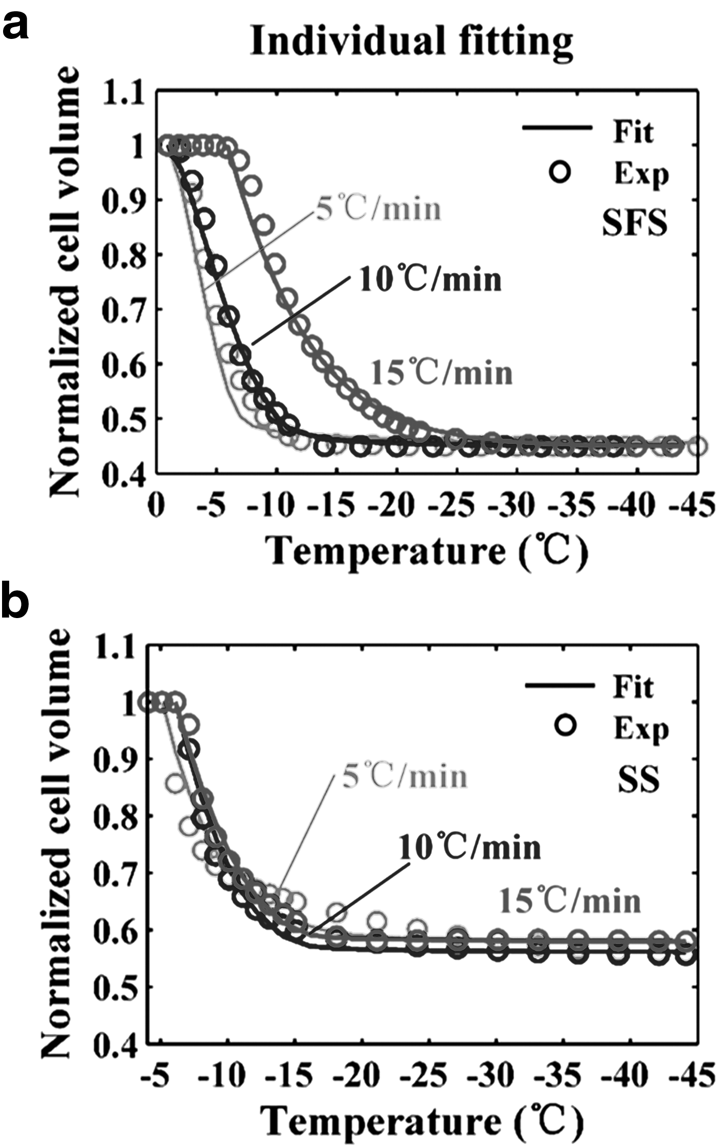
The partial and total thermogram differences between the initial and final slow cooling process were calculated using TA Universal Analysis software. The cell volume at temperature T, V(T), during cooling was determined according to Equation (1). All of thermogram for three cooling rates are shown in Supplementary Figure S1. (Supplementary materials are available online at www.liebertpub.com/bio). The volumetric response of HeLa cells at 5°C/min, 10°C/min, and 15°C/min was expressed as normalized cell volume (V(T)/V_o) and represented as circles in Figure 1a. The temperature range was only shown in the range from 0 to −45°C, because the whole dynamic water transport process is included in this range. Cells cooled at 5°C/min and 10°C/min underwent rapid dehydration between about −1°C and −12°C during the initial phase of the cooling process. The dynamic portion of the cooling curve for cells that cooled at 15°C/min is between about −6°C and −20°C. With the temperature decreasing, the water transport was asymptotically stable and the normalized cell volume approached a constant value.

FIG. 1.

Volumetric response of HeLa cells obtained using the SFS cooling method (a) and the SS cooling method (b), respectively. The measured volumetric response is shown as circles, whereas the individual fitted dynamic response is shown as solid lines. SFS, slow-fast-slow; SS, single-slow.

Volumetric response of HeLa cells measured by the SS cooling protocol

The heat release at temperature T, q(T), was calculated using TA Universal Analysis software. Furthermore, linear fitting of q(T) and cytocrits, α, was obtained.

The volumetric response of HeLa cells was determined as described in Equations (2) and (3). The results are expressed as normalized cell volume (V(T)/V_o) and shown as circles in Figure 1b. The dynamic portion of the cooling process is between about −5°C and −30°C, −6°C and −17°C, and −7°C and −20°C at the cooling rate of 5°C/min, 10°C/min, and 15°C/min, respectively.

The hydraulic conductivity and activation energy of the cell membrane

The water transport model [Eqs. (5) and (6)] was used to simulate L_pg (the cell membrane hydraulic conductivity at reference temperature T_R, 273.15K) and E_Lp (the activation energy of L_pg).

An individual curve-fitting method was applied to fit the water transport model to the cell volume data measured at each cooling rate, and the corresponding fitting curves of the SFS and SS method are shown as solid lines in Figure 1a and b, respectively. The individual fit of the water transport model to the cell volume data measured by the SFS method was obtained for hydraulic conductivity values of L_pg = 0.11 ± 0.02 μm/(min·atm) and E_Lp = 27.2 ± 0.8 kcal/mol with R² > 95, whereas the corresponding values for the SS method were L_pg = 0.14 ± 0.04 μm/(min·atm) and E_Lp = 35.4 ± 7.0 kcal/mol with R² > 93 (Table 2). In addition, reference data of HeLa cells obtained by the cryomicroscopy method²³ and the SFS method¹⁵ are listed in Table 2 for comparison.

Table 2.

Membrane Permeability Parameters and Activation Energy Obtained from Individual Curve Fitting, and Predicted Optimal Rates of Freezing for HeLa Cells

	L_pg (μm/(min·atm))		E_Lp (kcal/mol)		V_b/V_o		R² (%)
Method	Indiv.	Comb.	Indiv.	Comb.	Indiv.	Comb.	Indiv.	Comb.	B_opt
SFS	0.11 ± 0.02	0.10	27.2 ± 0.8	22.9	0.42 ± 0.05	0.44	>95	97	19.6
SS	0.14 ± 0.04	0.10	35.4 ± 7.0	23.6	0.51 ± 0.09	0.58	>93	92	19.4
Cryo-microscopy²³	0.15 ± 0.05	0.140	6.4 ± 1.4	17.29	0.38 ± 0.08	0.38	>96		—
SFS¹⁵	0.08		10.9		0.45		>99		30.6

The fitting method was not specified in Ref.¹⁵

Comb., Combined; Indiv., Individual.

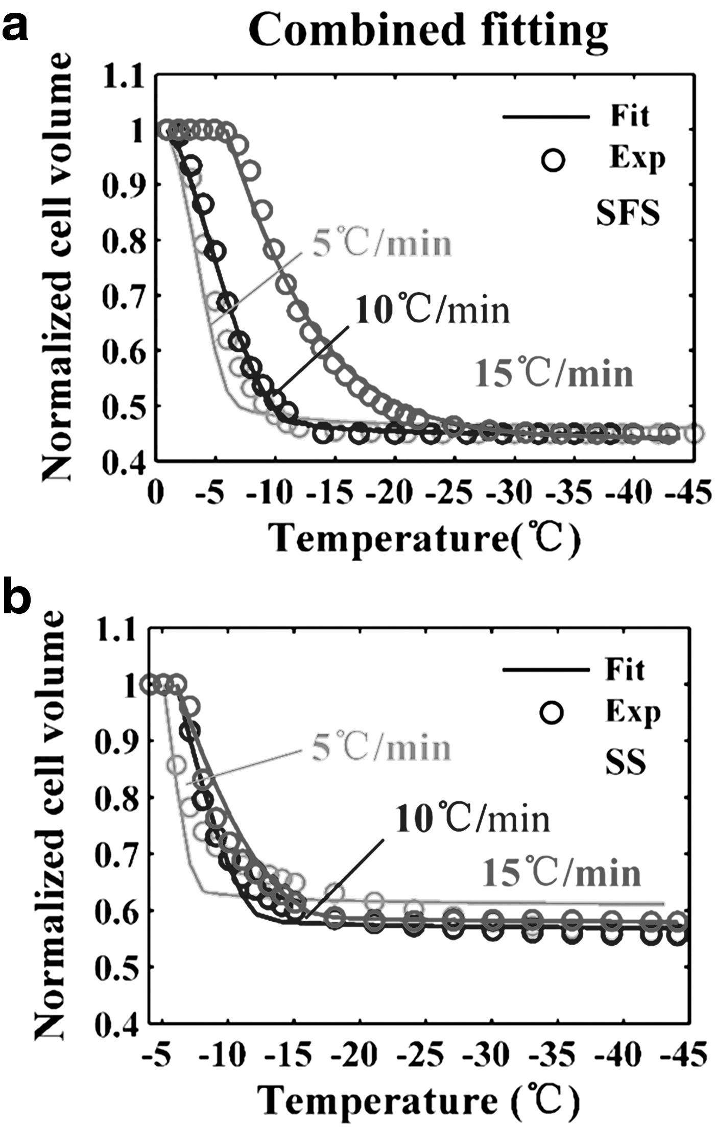
The cell heterogeneity and employment of different cooling rates might induce errors in measuring the hydraulic conductivity and activation energy of HeLa cells. To reduce the possible errors induced by the cell heterogeneity and eliminate the effect of different cooling rates on results, the cell volumes at different cooling rates were pooled together simultaneously to conduct a combined fitting.²⁴ The goodness of fit, R², for three cooling rates was maximized concurrently by the combined fitting. The combined fitting curves of the two methods are shown as solid lines in Figure 2a and b. The combined fit of the water transport model to cell volume data measured by the SFS method was obtained for hydraulic conductivity values of L_pg = 0.10 μm/(min·atm) and E_Lp = 22.9 kcal/mol with R² = 97, whereas the corresponding values by the SS method were L_pg = 0.10 μm/(min·atm) and E_Lp = 23.6 kcal/mol with R² = 92 (Table 2).

FIG. 2.

Volumetric response of HeLa cells obtained using the SFS cooling method (a) and the SS cooling method (b), respectively. The measured volumetric response is shown as circles, whereas the combined fitted dynamic response is shown as solid lines.

Theoretically predicted optimal cooling rates

The values of theoretically predicted optimal cooling rates calculated according to Equation (7) are listed in Table 2. The predicted optimal cooling rate for HeLa cells obtained according to the SFS method is 19.6°C/min, and that according to the SS method is 19.4°C/min.

Simulation of cell volume change at the predicted optimal cooling rate according to results obtained by the SFS and the SS cooling methods is shown in Figure 3A and B, respectively. The simulation was also applied to cooling rates of 1°C/min, 30°C/min, 60°C/min, and 100°C/min for comparison.

FIG. 3.

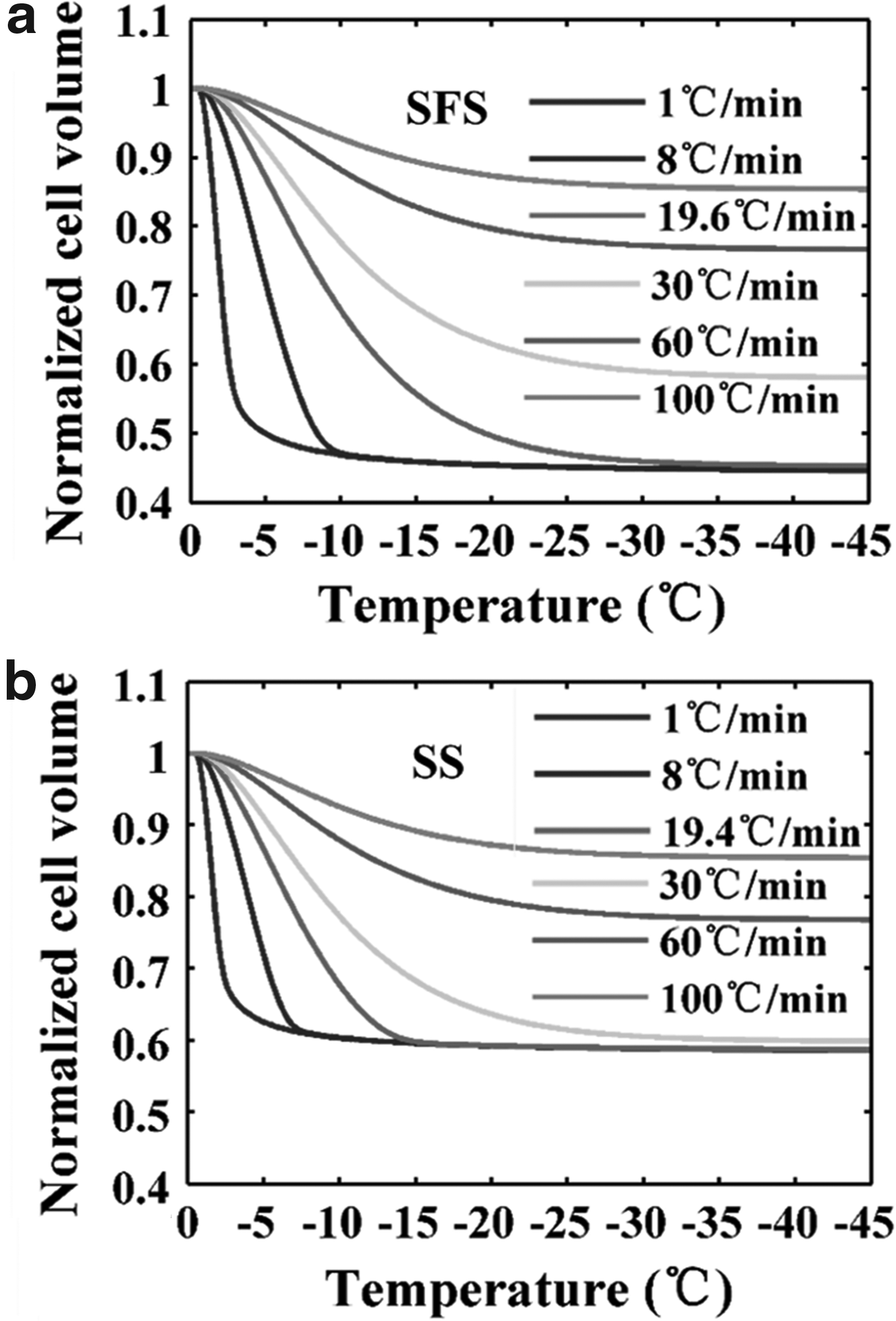
Predicted subzero transport of HeLa cells cooled at 1°C/min, 8°C/min, 30°C/min, 60°C/min, 100°C/min, and B_opt according to parameters obtained using the SFS cooling method (a) and the SS cooling method (b) by combined fitting, respectively.

Verification of simulation

To verify the results of simulation of cell volume change based on the parameters obtained by DSC data, a faster cooling rate (18°C/min) was used to compare the theoretically predicted and experimentally measured water transport behavior. This faster cooling rate is chosen as the fastest rate available considering the limitation in refrigeration capacity of refrigeration system of experimental apparatus (Supplementary Fig. S2). Since the results obtained by the SS method showed that the differences between different cooling rates were not significant, the SFS method was used in the verification experiment. As shown in Supplementary Figure S3, there is no change in gradient of heat flow curve during the initial cooling, which indicates no intracellular ice information. Figure 4 shows the water transport data and simulation using the combined fitting parameters (L_pg = 0.10 μm/(min·atm) and E_Lp = 22.9 kcal/mol) at a cooling rate of 18°C/min. It shows that the water transport behavior measured by the SFS method is in good agreement with the results of simulation.

FIG. 4.

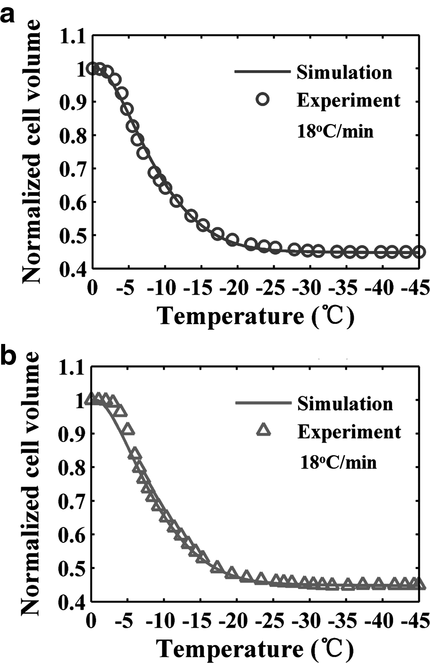
Volumetric response of HeLa cells cooled at 18°C/min. (a, b) Represent data obtained from sample 1 and sample 2, respectively. The model simulated response is shown as solid lines. Experimental data obtained from sample 1 and sample 2 are shown as circles and triangles, respectively.

Discussion

By comparison of the results measured by the SFS cooling protocol, there is a significant difference in the onset temperature and the range of volume change between 5°C/min and 15°C/min, 10°C/min and 15°C/min. It seems that HeLa cells underwent incomplete dehydration at 15°C/min. Unfortunately, we have no available means to verify the intracellular ice formation in cells cooled at 15°C/min. However, one can find that HeLa cells did not exhibit intracellular ice at the cooling rate of 15°C/min according to the study by Yi et al.²³ This is further supported by the observation that no secondary heat release was observed to indicate intracellular ice formation at 15°C/min. Therefore, it was supposed that HeLa cells underwent a great degree of dehydration at a cooling rate below 15°C/min, and this is in accord with the assumptions of the SFS cooling method.⁷ As shown in Figures 1a and 2a, there is a significant difference in the change of normalized cell volume at different cooling rates. This difference indicated the dependence of the water transport process on cooling rate and generally is in accord with the theory of cryobiology. Furthermore, the imitative effect of both individual fit and combined fit for the SFS method was better than that for the SS method. By comparison with the SFS cooling method, the cell volume shrinkage obtained from the SS cooling method was markedly different at each cooling rate. The onset temperature was lower, and the range of dynamic water transport was wider. In Figure 1b, the dynamic water transport mainly occurred in the range of −6°C to −20°C at a cooling rate of 10°C/min and 15°C/min; whereas at the cooling rate of 5°C/min, the dynamic process started at about −5°C and lasted until about −30°C. The temperature range of dynamic water transport at 5°C/min was significantly wider than that at 10°C/min and 15°C/min, and it did not conform to the laws of cell volume change at different cooling rates.

FIG. 5.

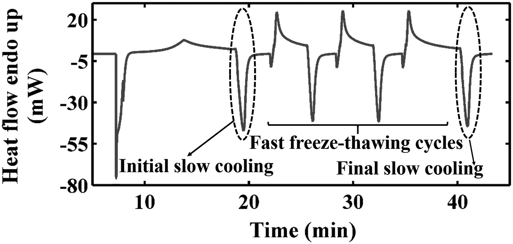
Experimental procedures of the SFS cooling method on DSC. DSC, differential scanning calorimetry.

From the results of individual fitting for the SS method shown in Figure 1b, there was no distinct difference in the change of normalized cell volume between 5°C/min, 10°C/min, and 15°C/min. However, as shown in Figure 2b, the results of combined fitting of the SS method indicated that the changes of normalized cell volume under different cooling rates are different from each other. This indicated the dependence of the water transport process on cooling rate. The imitative effect of the results obtained at 5°C/min was not as good as that at the other two cooling rates and the goodness of combined fit, and R², was only 92%. It was significantly lower than the goodness of combined fit of the SFS method, which was 97%. Nevertheless, the measurements were done at only one cooling rate in the previous study using the SS method.^16–19 Therefore, a comparison of the volumetric response of cells at different cooling rates was not possible.

FIG. 6.

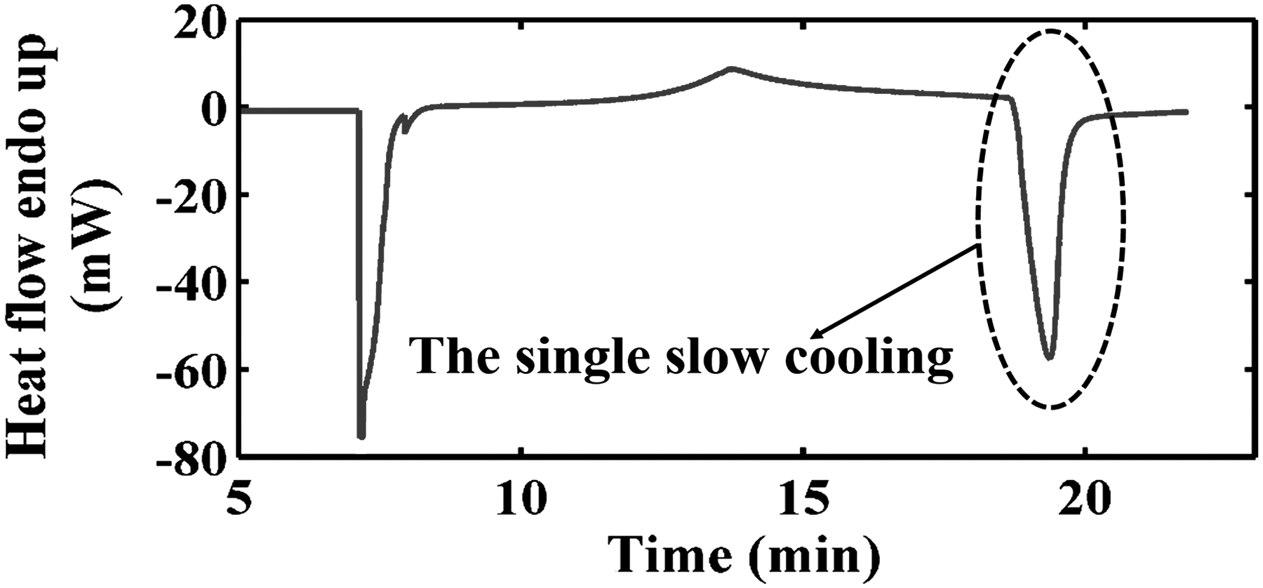
Experimental procedures of the SS cooling method on DSC.

FIG. 7.

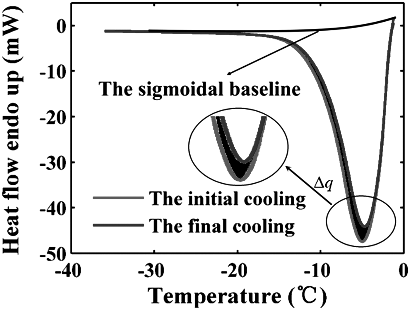
Comparison of heat flow obtained from the initial and the final cooling run (the representative data of 10°C/min).

Individual fitting results are shown in Table 2. Values of L_pg measured by two methods at each cooling rate were similar, whereas values of E_Lp measured by the SS method were about 30.1% more than values measured by the SFS method on average. However, the combined fitting results of L_pg and E_Lp from two methods were similar; therefore, the predicted optimal cooling rates were also very close. The reference values of L_pg ranged from 0.08 to 0.23 μm/(min·atm), whereas the values of E_Lp ranged from 10.9 to 37.4 kcal/mol.¹³ Therefore, our results obtained by the SFS and SS methods were comparable to previous studies and in a reasonable range (Table 2). What is more, Figure 4 shows that the experimental data should be basically in accord with the simulative data. It indicates that the model parameters can predict the water transport data effectively.

In addition, the inactive volume, V_b, obtained from the SFS and SS cooling methods by combined fitting is 0.44 and 0.58, respectively. These two values are comparable, and the variation might be due to limited sampling. However, there is a difference between the value of inactive cell volume and the published value of V_b = 0.38V_o by Yi and Zhao²³ and V_b = 0.38V_o by Morrill and Robbins.²⁵ These differences in inactive cell volumes might be caused by the different growth conditions employed for HeLa cells.

FIG. 8.

The linear functions of the partial heat release per unit mass of suspensions and cytocrits at different temperatures (the representative data of 10°C/min).

Factors accounting for the differences of results between two methods

Besides some disadvantages and limitations of the DSC technique concluded by Devireddy et al.,⁷ factors accounting for the differences between results measured by the SFS and SS cooling protocols can be classified by the following points:

(i) Sample non-homogeneity

In each DSC experiment, only a small droplet of cell suspension was used; hence, the concentration of Pseudomonas syringae may be different for each sample. This may cause differences in freezing points and heat release, so it is difficult to guarantee the exact consistency of samples.

(ii) The instability of purge gas flow

The purge gas flow in DSC was unstable. This may effect heat transfer between furnace and crucible and may cause a slight inaccuracy in heat flow.

(iii) Temperature gradient

The mass of each sample was controlled in the range of 5 to 10 mg. Any temperature gradient produced in a sample may cause deviation between indicated and actual sample temperature. The mass of the sample should be as small as possible to avoid excessive temperature gradient and improve experimental accuracy.

(iv) Constant cooling rate not guaranteed

The cooling attachment of DSC used in this study was the mechanical refrigeration type. Though the cooling rate of 15°C/min might exceed the maximum cooling capacity of the instrument, the analysis of temperature change curves of samples shows that the cooling rate was in close proximity of 15°C/min. However, it decreased when the sample experienced phase transformation from liquid to crystal, because the cooling attachment could not provide enough cold energy to compensate for the heat release of the sample due to phase change. However, the cooling rate was regarded as constant in data processing, which is not the case in practice. The deviation of the nominal and actual cooling rate during phase change may introduce an error to the results.

(v) Heat flow curve overlap

In the SFS cooling method, the heat flow measured in the initial cooling process should be less than that measured in the final cooling process, (q_initial < q_final). But in fact, these two heat flow curves overlap at the beginning of cooling. Therefore, the difference of heat flow between the initial and final process might be very small, even negative. The heat flow difference curves fluctuated at the initial stage of slow cooling. Only by smooth processing by thermal analysis software can the difference curves be integrated effectively. Studies on the human dermal fibroblasts using the SFS cooling protocol show that initial and final heat flow curves often overlapped.¹⁴ Furthermore, the integrated value of the total difference between the initial and final heat flow curves was too small to be significant (±5 J/g), as is the case for human erythrocytes and yeast cells.¹⁸ According to an analysis by Han et al.,¹⁸ what may cause an unsatisfactory result of this method is that the fast freeze-thawing cycle cannot ensure damaged cells, especially for some cell types where the membrane may reseal during thawing and cells with a cell wall to protect the membrane from intracellular ice formation. These findings indicate that the SFS cooling method has some inaccuracies and may not be applicable to every cell system.

Comparison of the SFS and the SS cooling method

Though the SS cooling protocol modified and simplified the temperature program of DSC experiments, this method needs samples with different cytocrits to obtain results. Thus, it complicates sample preparation and increases experimental time. However, the SFS cooling method has no requirement with regard to cytocrits. But samples with the same cytocrit were used in these studies. Since data processing can be done on results from a single sample, the experimental time of the SFS cooling method is relatively short, though the temperature program of each sample is somewhat cumbersome.

Conclusions

The values of the hydraulic conductivity and activation energy of HeLa cells were comparable. These two methods obtained the same hydraulic conductivity values and similar activation energy values according to combined fitting results. In the SFS method, each sample was cooled at a slow rate initially and then damaged by fast freeze-thawing cycles. Finally, the sample was cooled at the same slow cooling rate as initially. The differences between the two slow cooling rates were calculated to obtain the hydraulic conductivity and activation energy. An analysis can be conducted on a single sample. In the SS method, SS cooling was employed for each sample; however, samples with different cytocrits were required for analysis and more experimental time was required.

Footnotes

Acknowledgment

This work was partially supported by grants from NSFC (Nos. 20803016, 51476160, and 51528601). We thank Bo Jin for providing technical support.

Author Disclosure Statement

No conflicting financial interests exist.

References

Mazur

. Freezing of living cells: Mechanisms and implications. Am J Physiol, 1984; 247:C125–C142.

Gao

, Critser

J K

. Mechanisms of cryoinjury in living cells. ILAR J, 2000; 41:187–196.

Mazur

. Equilibrium, quasi-equilibrium, and nonequilibrium freezing of mammalian embryos. Cell Biophys, 1990; 17:53–92.

Mazur

. Cryobiology: The freezing of biological systems. Science, 1970; 168:939–949.

Shabana

, Mcgrath

. Cryomicroscope investigation and thermodynamic modeling of the freezing of unfertilized hamster ova. Cryobiology, 1988; 25:338–354.

Diller

. Quantitative low-temperature optical microscopy of biological-systems. J Microsc, 1982; 126:9–28.

Devireddy

, Raha

, Bischof

. Measurement of water transport during freezing in cell suspensions using a differential scanning calorimeter. Cryobiology, 1998; 36:124–155.

Devireddy

, Swanlund

, Roberts

. Bischof

J.C.

Subzero water permeability parameters of mouse spermatozoa in the presence of extracellular ice and cryoprotective agents. Biol Reprod, 1999; 61:764–775.

Devireddy

, Swanlund

, Roberts

, et al. The effect of extracellular ice and cryoprotective agents on the water permeability parameters of human sperm plasma membrane during freezing. Hum Reprod, 2000; 15:1125–1135.

10.

Devireddy

, Coad

, Bischof

. Microscopic and calorimetric assessment of freezing processes in uterine fibroid tumor tissue. Cryobiology, 2001; 42:225–243.

11.

Devireddy

, Swanlund

, Olin

, et al. Cryopreservation of equine sperm: Optimal cooling rates in the presence and absence of cryoprotective agents determined using differential scanning calorimetry. Biol Reproduct, 2001; 66:222–231.

12.

Thirumala

, Ferrer

, Al-Jarrah

, et al. Cryopreservation of canine spermatozoa: Theoretical prediction of optimal cooling rates in the presence and absence of cryoprotective agents. Cryobiology, 2003; 47:109–124.

13.

Alapati

, Goff

, Kubisch

, et al. Water transport in epididymal and ejaculated rhesus monkey (Macaca mulatta) sperm during freezing. Cryobiology, 2008; 57:182–185.

14.

Mori

, Choi

, Devireddy

, et al. Calorimetric measurement of water transport and intracellular ice formation during freezing in cell suspensions. Cryobiology, 2012; 65:242–255.

15.

Thirumala

, Forman

, Monroe

. Devireddy

. Freezing and post-thaw apoptotic behaviour of cells in the presence of palmitoyl nanogold particles. Nanotechnology, 2007; 18:195104.

16.

Luo

, Han

, He

, et al. A modified differential scanning calorimetry for determination of cell volumetric change during the freezing process. Cryoletters, 2002; 23:229–236.

17.

Armitage

. Effect of solute concentration on intracellular water volume and hydraulic conductivity of human-blood platelets. J Physiol, 1986; 374:375–385.

18.

Han

, Luo

, Cui

, et al. A modified differential scanning calorimetry method for determining water transport properties in biological cells during the freezing process. Cell Preserv Technol, 2007; 5:25–32.

19.

Zhao

, He

, Guo

. Comparison study of trapped water in human erythrocytes by EPC and DSC method and its application. Sci China Ser E, 2004:343–351.

20.

Mazur

. Kinetics of water loss from cells at subzero temperatures and likelihood of intracellular freezing. J Gen Physiol, 1963; 47:347–369.

21.

Levin

, Cravalho

, Huggins

. Membrane model describing effect of temperature on water conductivity at subzero temperatures. Cryobiology, 1976; 13:415–429.

22.

Thirumala

, Devireddy

. A simplified procedure to determine the optimal rate of freezing biological systems. J Biomech Eng, 2004; 127:295–300.

23.

, Zhao

. Effect of hydroxyapatite nanoparticles on biotransport phenomena in freezing HeLa cells. J Nanotechnol Eng Med, 2014; 5:040904-1-040904-7.

24.

Berrada

, Bischof

. Evaluation of freezing effects on human microvascular-endothelial cells (HMEC). Cryobiology, 2001; 22:353–366.

25.

Morrill

, Robbins

. Changes in intracellular cations during the cell cycle in HeLa cells. Physiol Chem Phys Med NMR, 1984; 16:209–219.

Supplementary Material

Please find the following supplemental material available below.

For Open Access articles published under a Creative Commons License, all supplemental material carries the same license as the article it is associated with.

For non-Open Access articles published, all supplemental material carries a non-exclusive license, and permission requests for re-use of supplemental material or any part of supplemental material shall be sent directly to the copyright owner as specified in the copyright notice associated with the article.

0.26 MB

0.07 MB

0.00 MB

0.06 MB