Measurement of Thermal Conductivities of Two Cryoprotective Agent Solutions for Vitreous Cryopreservation of Organs at the Temperature Range of 77 K–300 K Using a Thermal Sensor Made of Microscale Enamel Copper Wire

Abstract

Biobanking of organs by cryopreservation is an enabling technology for organ transplantation. Compared with the conventional slow freezing method, vitreous cryopreservation has been regarded to be a more promising approach for long-term storage of organs. The major challenges to vitrification are devitrification and recrystallization during the warming process, and high concentrations of cryoprotective agents (CPAs) induced metabolic and osmotic injuries. For a theoretical model based optimization of vitrification, thermal properties of CPA solutions are indispensable. In this study, the thermal conductivities of M22 and vitrification solution containing ethylene glycol and dimethyl sulfoxide (two commonly used vitrification solutions) were measured using a self-made microscaled hot probe with enameled copper wire at the temperature range of 77 K–300 K. The data obtained by this study will further enrich knowledge of the thermal properties for CPA solutions at low temperatures, as is of primary importance for optimization of vitrification.

Introduction

Cryopreservation is an important technique for preserving cells and organs by cooling to very low temperatures (typically −196°C using liquid nitrogen). Traditional techniques of cryopreservation are slow freezing and vitrification, and both are currently used in practical applications.¹ For the former, cells are usually cooled in the presence of cryoprotectant (concentration of 1–2 mol/L) at a slow cooling rate (typically less than 5°C·min⁻¹). The slow cooling rate allows the cells to dehydrate by maintaining equilibrium with the partially frozen extracellular space, as freezing can cause significant damage to cells.^2–4 For the latter, cells are pipetted into a medium that has very high concentrations of cryoprotective agents (CPAs) and finally reach the amorphous glass state without crystallization at the applied cooling rate. Therefore, samples can be cryopreserved without any detrimental intracellular ice formation.^5–8 When cells are exposed to high concentrations of CPAs, osmotic and toxic injuries of cells or organs can occur and reduce the viability of cell by destroying cell membranes and cell morphology.^9–12

Vitrification has been found to be a reliable and effective method for preservation of cells/tissues and organs.^6,13,14 The role of CPAs is to minimize or prevent cells or tissues from being damaged during exposure to low temperature. CPAs can be divided into two main groups based on their role in cryopreservation. The first one is penetrable CPAs, which can penetrate the cell membrane during vitrification or slow freezing, such as dimethyl sulfoxide (DMSO), glycerol, ethylene glycol (EG), and 1,2-propanediol. The other category is nonpenetrable CPAs, which cannot penetrate the cell membrane due to large molecular weight. Typically, nonpenetrable CPAs contain some large molecular weight polymers and sugars such as polyvinylpyrrolidone, polyethylene glycol, and sucrose.^15–18 Many investigations have been reported on usage of individual cryoprotectant agents in cell preservation, and the combination of two or more different CPAs can significantly reduce cell toxicity and osmotic stress.^7,14,19 For example, VS1,²⁰ VS4,²¹ VS55,^22–24 and M22²⁵ are combinations of various CPAs, which have notable protective effects on cells/tissues and organs during cryopreservation.

Many studies have been conducted on the measurement of thermal conductivity and thermal diffusivity using both transient heat wire^26–28 and hot probe methods.^29–32 It has been found that the use of the transient heat wire technique is more accurate, although it has some limitations in the measurement of liquids and powders, whereas the hot probe method is a significant improvement. The hot probe is made up of microsize metal copper wires with embedded ethoxyline and protected by a stainless steel tube of needles for inserting into soft samples. Ethoxyline is used to fill the space between the heater (copper wire) and the tube during fabrication and to improve the heat conduction inside the probe. The copper wire acts as an electric heater and thermistor/sensor simultaneously, which provides uniform heating inside the probe.

In this work, we established an accurate experimental-modeling approach to analyze the vitrification process along with the thermal properties of different vitrification solutions. The thermal conductivities of M22²⁵ and vitrification solution containing ethylene glycol and dimethyl sulfoxide (VSED)²¹ were measured using a self-made microscaled hot probe made of enameled copper wire at the temperature range of 77 K–300 K. The hot probe is calibrated with water and 29.9 wt% of CaCl₂ aqueous solution. These results enrich the thermal conductivity data over the temperature range of 77 K–300 K, which can be used in the future cryopreservation model.

Model Analysis

Theoretical model

The governing equation along with initial conditions of the model can be described as follows, to explain the thermal conductivity properly. The hot probe is inserted into the solution for measuring thermal conductivity as a constant heating substance with infinite length and has a radius of r₀ to conduct sporadically with infinite medium. \documentclass{aastex}\usepackage{amsbsy}\usepackage{amsfonts}\usepackage{amssymb}\usepackage{bm}\usepackage{mathrsfs}\usepackage{pifont}\usepackage{stmaryrd}\usepackage{textcomp}\usepackage{portland, xspace}\usepackage{amsmath, amsxtra}\pagestyle{empty}\DeclareMathSizes{10}{9}{7}{6}\begin{document} \begin{align*} \begin{cases} \begin{matrix} { \frac { \partial T } { \partial \tau } } = \frac { \alpha } { r } \frac { \partial } { { \partial r } } \left( { r { \frac { \partial T } { \partial r } } } \right) \ , \ ( \tau > 0 , { r_0 } < r < + \infty ) \hfill \\ { \rm { \pi } } r_0^2 { \rho _w } { c_w } { \frac { \partial { T_w } } { \partial \tau } } = q + 2 \pi \lambda { r_0 } { \frac { \partial T } { \partial r } } \vert { _ { r = r_0^ + } } \hfill \\ T = { T_0 } , ( r \to \infty , \tau \ge 0 ) \hfill \\ T = { T_0 } , ( r \ge 0 , \tau = 0 ) \hfill\end{matrix} \end{cases} \tag { 1 }\end{align*} \end{document}

where T(K) is the temperature; τ(s) is the heating time; q (W · s⁻¹) = I²R/L is the heating power per effective length of the probe; ρ(kg·m³) and c(J·[kg·K]⁻¹) are the density and thermal capacity of the material, respectively; α (m²·s⁻¹) and λ(W[m·K]⁻¹) are the thermal diffusivity and thermal conductivity of the measured samples, and the subscript w is expressed as the hot probe property.

After solving the model equation, we obtained the following result.³³ \documentclass{aastex}\usepackage{amsbsy}\usepackage{amsfonts}\usepackage{amssymb}\usepackage{bm}\usepackage{mathrsfs}\usepackage{pifont}\usepackage{stmaryrd}\usepackage{textcomp}\usepackage{portland, xspace}\usepackage{amsmath, amsxtra}\pagestyle{empty}\DeclareMathSizes{10}{9}{7}{6}\begin{document} \begin{align*} \theta \left( { \rm T } \right) = { \frac { 2q \omega } { { \pi ^3 } { \lambda _0 } } } \mathop \int \limits_0^ \infty { \frac { 1 - \exp \left( { - { \frac { \alpha t } { r_0^2 } } } \right) } { { u^3 } \Delta \left( { u , \omega } \right) } } du \tag { 2 } \end{align*} \end{document}

where \documentclass{aastex}\usepackage{amsbsy}\usepackage{amsfonts}\usepackage{amssymb}\usepackage{bm}\usepackage{mathrsfs}\usepackage{pifont}\usepackage{stmaryrd}\usepackage{textcomp}\usepackage{portland, xspace}\usepackage{amsmath, amsxtra}\pagestyle{empty}\DeclareMathSizes{10}{9}{7}{6}\begin{document} $\Delta u ( u , \omega ) = { \left[ {u{J_0} ( u ) - \omega {J_1} ( u ) } \right] ^2} + { \left[ {u{Y_0} ( u ) + \omega {Y_1} ( u ) } \right] ^2}$ \end{document} , J₀(u) and J₁(u) are the zero-order and first-order Bessel function of the initial kind or first kind, respectively; Y₀(u) and Y₁(u) are the zero-order and first-order Bessel function of the second kind, respectively; \documentclass{aastex}\usepackage{amsbsy}\usepackage{amsfonts}\usepackage{amssymb}\usepackage{bm}\usepackage{mathrsfs}\usepackage{pifont}\usepackage{stmaryrd}\usepackage{textcomp}\usepackage{portland, xspace}\usepackage{amsmath, amsxtra}\pagestyle{empty}\DeclareMathSizes{10}{9}{7}{6}\begin{document} $\omega = {2} \rho {\rm {c}} {/} ( \rho_{w} c_{w}) $ \end{document} is the heat capacity ratio; θ(T) = T − T₀ is the surface temperature rise of hot probe; and T₀ is the initial temperature.

If the model equation satisfied the condition which was \documentclass{aastex}\usepackage{amsbsy}\usepackage{amsfonts}\usepackage{amssymb}\usepackage{bm}\usepackage{mathrsfs}\usepackage{pifont}\usepackage{stmaryrd}\usepackage{textcomp}\usepackage{portland, xspace}\usepackage{amsmath, amsxtra}\pagestyle{empty}\DeclareMathSizes{10}{9}{7}{6}\begin{document} $ { \frac { r_0^2 } { 4 \alpha \tau } } < < 1$ \end{document} ³³ then we get the following simplified equation using series expansion and neglect high-order terms of the equation (2) for describing the thermal conductivity. \documentclass{aastex}\usepackage{amsbsy}\usepackage{amsfonts}\usepackage{amssymb}\usepackage{bm}\usepackage{mathrsfs}\usepackage{pifont}\usepackage{stmaryrd}\usepackage{textcomp}\usepackage{portland, xspace}\usepackage{amsmath, amsxtra}\pagestyle{empty}\DeclareMathSizes{10}{9}{7}{6}\begin{document} \begin{align*} {\rm {\lambda}} = {\frac {q} {4 \pi}} {\bigg {/}} {\frac {d \theta} {dlnt}} \tag {3} \end{align*} \end{document}

The dependence of the thermal resistance of copper material on temperature could be written as follows³²: \documentclass{aastex}\usepackage{amsbsy}\usepackage{amsfonts}\usepackage{amssymb}\usepackage{bm}\usepackage{mathrsfs}\usepackage{pifont}\usepackage{stmaryrd}\usepackage{textcomp}\usepackage{portland, xspace}\usepackage{amsmath, amsxtra}\pagestyle{empty}\DeclareMathSizes{10}{9}{7}{6}\begin{document} \begin{align*} {{ \rm{R}}_t} = {R_0} \left[ {1 + { \beta _0} \left( {T - {T_0}} \right) } \right] \; \tag{4} \end{align*} \end{document} \documentclass{aastex}\usepackage{amsbsy}\usepackage{amsfonts}\usepackage{amssymb}\usepackage{bm}\usepackage{mathrsfs}\usepackage{pifont}\usepackage{stmaryrd}\usepackage{textcomp}\usepackage{portland, xspace}\usepackage{amsmath, amsxtra}\pagestyle{empty}\DeclareMathSizes{10}{9}{7}{6}\begin{document} \begin{align*} \Delta { \rm{R}} = \left( {{ \beta _0}{R_0}} \right) \Delta T \tag{5} \end{align*} \end{document}

where R_t and R₀ represent the resistances corresponding to the temperatures T and T₀, respectively; β₀ is a coefficient at T₀; and the \documentclass{aastex}\usepackage{amsbsy}\usepackage{amsfonts}\usepackage{amssymb}\usepackage{bm}\usepackage{mathrsfs}\usepackage{pifont}\usepackage{stmaryrd}\usepackage{textcomp}\usepackage{portland, xspace}\usepackage{amsmath, amsxtra}\pagestyle{empty}\DeclareMathSizes{10}{9}{7}{6}\begin{document} ${ \beta _0}{R_0}$ \end{document} is a constant for a certain probe.

Using the equation (2) after combining the Ohm's law as R = U/I and equation (4), we obtained the final equation for thermal conductivity as follows: \documentclass{aastex}\usepackage{amsbsy}\usepackage{amsfonts}\usepackage{amssymb}\usepackage{bm}\usepackage{mathrsfs}\usepackage{pifont}\usepackage{stmaryrd}\usepackage{textcomp}\usepackage{portland, xspace}\usepackage{amsmath, amsxtra}\pagestyle{empty}\DeclareMathSizes{10}{9}{7}{6}\begin{document} \begin{align*} {\rm {\lambda}}_{t} ={\rm CI^{3} R_{t}} {\bigg {/}} {\frac {dU} {dlnt}} \tag {6} \end{align*} \end{document}

where C represents the hot probe constant and is defined as \documentclass{aastex}\usepackage{amsbsy}\usepackage{amsfonts}\usepackage{amssymb}\usepackage{bm}\usepackage{mathrsfs}\usepackage{pifont}\usepackage{stmaryrd}\usepackage{textcomp}\usepackage{portland, xspace}\usepackage{amsmath, amsxtra}\pagestyle{empty}\DeclareMathSizes{10}{9}{7}{6}\begin{document} $C = {{ \beta _0}{R_0}} \mathord { \vphantom {{{ \beta _0}{R_0}} {64 \pi L}}} {64 \pi L}$ \end{document} of which \documentclass{aastex}\usepackage{amsbsy}\usepackage{amsfonts}\usepackage{amssymb}\usepackage{bm}\usepackage{mathrsfs}\usepackage{pifont}\usepackage{stmaryrd}\usepackage{textcomp}\usepackage{portland, xspace}\usepackage{amsmath, amsxtra}\pagestyle{empty}\DeclareMathSizes{10}{9}{7}{6}\begin{document} ${ \beta _0}{R_0}$ \end{document} is constant and L is the effective length of the probe; \documentclass{aastex}\usepackage{amsbsy}\usepackage{amsfonts}\usepackage{amssymb}\usepackage{bm}\usepackage{mathrsfs}\usepackage{pifont}\usepackage{stmaryrd}\usepackage{textcomp}\usepackage{portland, xspace}\usepackage{amsmath, amsxtra}\pagestyle{empty}\DeclareMathSizes{10}{9}{7}{6}\begin{document} ${{ \rm{ \lambda }}_{ \rm{t}}}$ \end{document} is the thermal conductivity at the target temperature T.

Data analysis protocol

The experimental results have been used in two data analysis protocols, namely the least square method (LSM) and the Monte Carlo inversion method (MCIM)³⁴ based on the equations (6) and (3), respectively. The hot probe constant was calibrated with water and 29.9% of CaCl₂ aqueous solution. Subsequently, the thermal conductivity of samples has been measured in this study. Characteristic fitting curves of both methods are shown in Figure 1a and b, respectively. A linear region occurred in the U/V-ln (t) curve as shown in Figure 1a and we also obtained the slope of linear portion using the LSM.

FIG. 1.

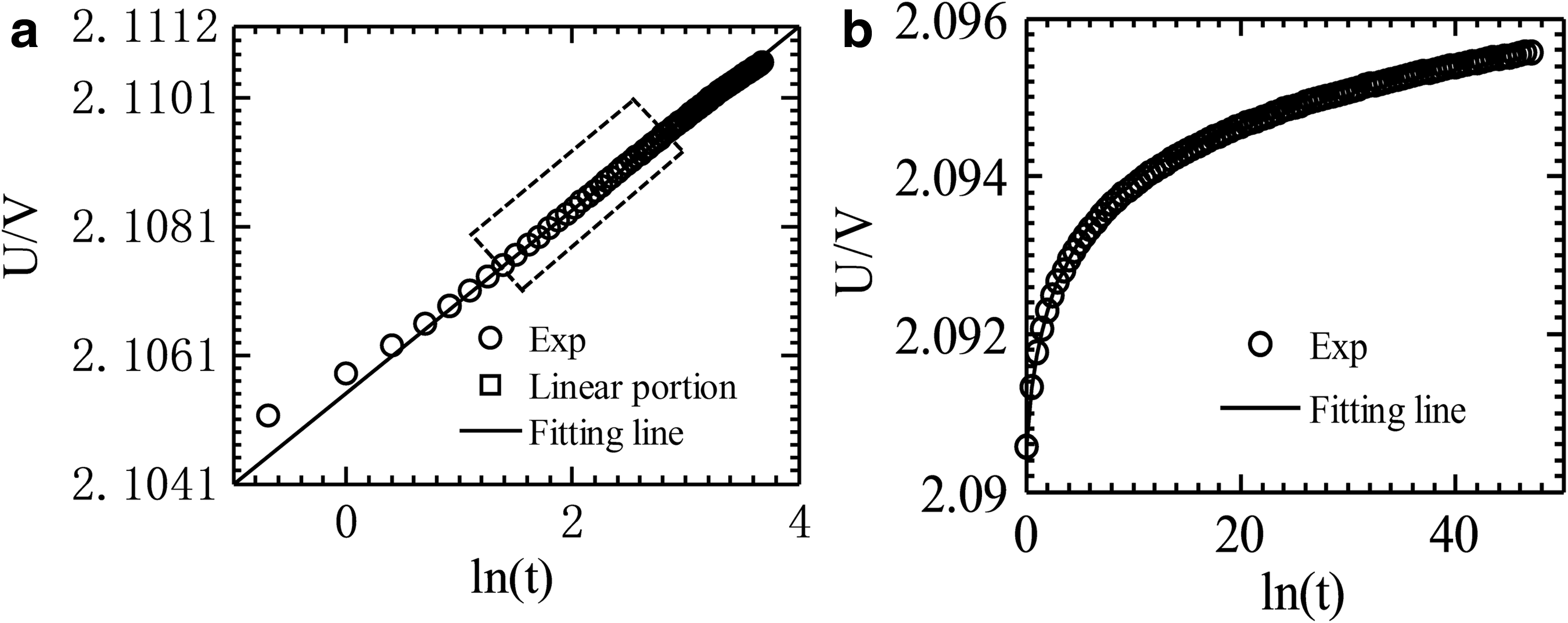
Characteristic fitting curve as (a) the LSM and (b) the MCIM. LSM, least square method; MCIM, Monte Carlo inversion method.

Consequently, the heat capacity and the effective length of the hot probe were calibrated with water and CaCl₂ aqueous solution. A series of stochastic “thermal conductivity λ” values are generated in a certain range using the computer, and the temperature rise curves are calculated by substituting them into the equation (3). Then the MCIM led to the comparison between the fitting curve and experimental curve as shown in Figure 1b. When the deviation between the simulated temperature rise curve and the experimental curve is the minimum, then the “thermal conductivity λ” value is what is needed. The procedure has been followed systematically until finding the concluding neighborhood with the MCIM, and we also repeated the techniques until acquiring the stable and precise response³⁴ in this scheme.

Experiments

The hot probe

The microscaled hot probe was made of enameled copper wires with embedded ethoxyline and protected by a stainless steel tube of needles for inserting into soft samples. The effective length of the stainless steel tube of needles was considered as 37 mm, and the needle's outer diameter and inner diameter were 0.82 and 0.51 mm, respectively. The diameter of enameled copper wire was 0.02 mm. The inner copper wire served as the electrical heater and temperature sensor simultaneously. There is almost 110 Ω resistance at room temperature for the enameled copper wire with 3 m in total length. We assumed that the surface temperature distribution of the probe is uniform because the thermal contact resistance in some places does not significantly affect the average temperature when using the copper wire as the temperature sensor in this study. The ethoxyline was used to fill the space of heater and outer tube layer during fabrication and enhanced the heat transfer inside the chamber of the probe as well.

Sample preparation

In this study, we focused our effort on two vitrification solutions, VSED and M22. All reagents were purchased from Sigma-Aldrich. VSED consisted of EG 1.61 mol/L and DMSO 1.28 mol/L, whereas M22 is a composite of DMSO 2.855 mol/L (22.3.5% w/v), formamide 2.855 mol/L (12.858% w/v), and EG 2.713 mol/L (15.83% w/v). The key components of these solutions have been prepared in our laboratory. It should be noted that the thermal conductivity of M22 and VSED cryoprotectants has not been reported successfully at low temperature.

Experimental system and measurement procedure

Figure 2 displays the schematic diagram of the experimental setup and the corresponding image to measure the thermal conductivity of solutions. Figure 2a shows data acquisition (Agilent 34970A), a SourceMeter (Keithley 2400), a low temperature bath (EYELA NCB-2400), a thermocouple (T type, copper–constantan), a vacuum flask immersed with ice water mixture, and a hot probe with a sample scaffolding. The stainless steel bucket cannot be reproduced in this figure due to its complex wiring structure.

FIG. 2.

Schematic diagram of (a) experimental composition and (b) photographic image.

In addition, the stainless steel bucket is wrapped with thermal insulation materials and contains the vitrification solution (M22 or VSED) during the experiment, while the container has been immersed in a circular barrel connecting with a low temperature bath (EYELA NCB-2400). The microscaled hot probe is also inserted into the sample solution to hold the solution at the targeted temperature in the circular barrel and low temperature bath. In addition, data acquisition (Agilent 34970A) was set to be an auto range of 6.5 digits that was used for the temperature monitor and the voltage scanning from a different acquiring channel. Once the sample reached a stable condition at the targeted temperature, the channel for the temperature monitor was turned off while collecting the voltage range result of the hot probe at the speed of 0.5 seconds per single point. The SourceMeter (Keithley 2400) supplied the appropriate current source to ensure the temperature of hot probe rise during test, which was about 0.4°C, that is, reduced the error as noted in the cited reference.³⁰ The vacuum flask ice water provided the cold junction reimbursement of thermocouple in this model.

Results and Discussions

Calibration and verification of hot probe constants

During the experiments, a water and CaCl₂ aqueous solution have been used to calibrate the hot probe constants, which are denoted as C and L_av. The thermophysical properties of pure water and CaCl₂ aqueous solution have been collected from the cited references.^35,36 It should be noted that C is determined by the properties of the probe, which can be obtained by calibrating the probe over the temperature range 253 K–300 K as quoted in reference.³² In addition, it is really difficult to measure the calibration constant throughout the temperature range (77 K–300 K) due to the incomplete data for the thermal conductivities of the reference samples. Therefore, we determined the calibration constants in the temperature range of 253 K–300 K in this study. Figure 3a and b depicts the calibration constant versus temperature using the LSM. It should be mentioned that all data points have been collected repeatedly up to five times in the same experimental conditions. It revealed that the mean value of C was about 0.726772, and the maximum deviation of C_av was below 2.5%, where C_av is the average of all samples.

FIG. 3.

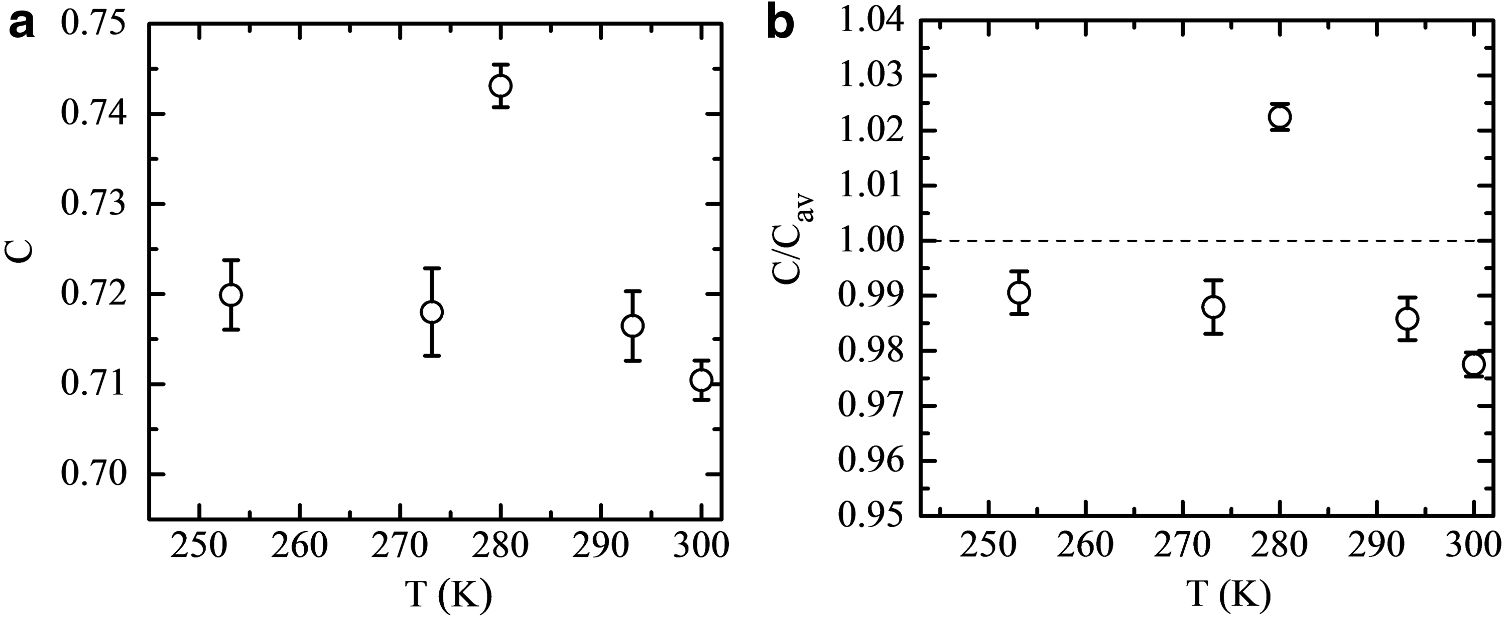
Calibration constant of the hot probe using LSM as (a) constant versus temperature profile and (b) C/C_av versus temperature profile.

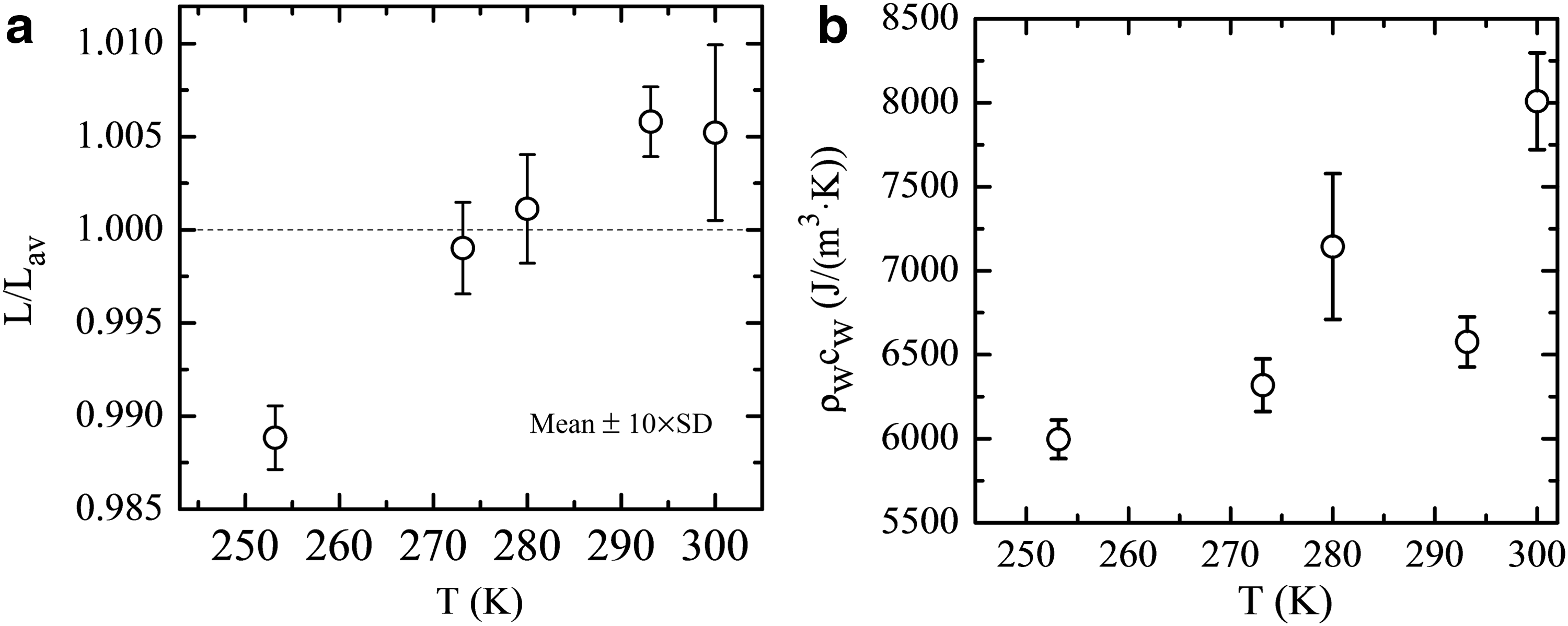
The calibration results versus temperature using the MCIM are illustrated in Figure 4. As shown in Figure 4a, the standard deviation of L_av was 1.116%, where L_av is the average value of the effective length of hot probe at the experimental temperature. The \documentclass{aastex}\usepackage{amsbsy}\usepackage{amsfonts}\usepackage{amssymb}\usepackage{bm}\usepackage{mathrsfs}\usepackage{pifont}\usepackage{stmaryrd}\usepackage{textcomp}\usepackage{portland, xspace}\usepackage{amsmath, amsxtra}\pagestyle{empty}\DeclareMathSizes{10}{9}{7}{6}\begin{document} ${ \rho _w}{c_w}$ \end{document} represented the heat capacity, which depends on temperature as shown in Figure 4b. It is notable that the calibration is necessary for all targeted temperatures, whereas the reference data were insufficient for certain temperatures in this work. As a result, there were some limitations for using the MCIM in this study.

FIG. 4.

Calibration of hot probe constant using MCIM as (a) L/L_av versus temperature profile and (b) ρ_wc_w versus temperature profile.

To verify the accuracy of the hot probe, we measured the thermal conductivity of DMSO aqueous solution (w = 0.5013) in this study. Table 1 presents the validation results for the sensor compared with the reference data as cited in reference.³⁷ It can be seen that the results of this work are in good agreement with those of the reference.

Table 1.

Verification Results of Hot Probe Using the Other Standard Solution Namely Dimethyl Sulfoxide Aqueous Solution (w = 0.5013) Comparing with the Reference Data

Temperature (K)	Reference value ³³	Experimental result	Deviation
280	0.319	0.3169999 ± 0.001738	−0.00627
290	0.324	0.330903 ± 0.002983	0.0213
300	0.33	0.340985 ± 0.000406	0.03329

Experiment results of M22 and VSED

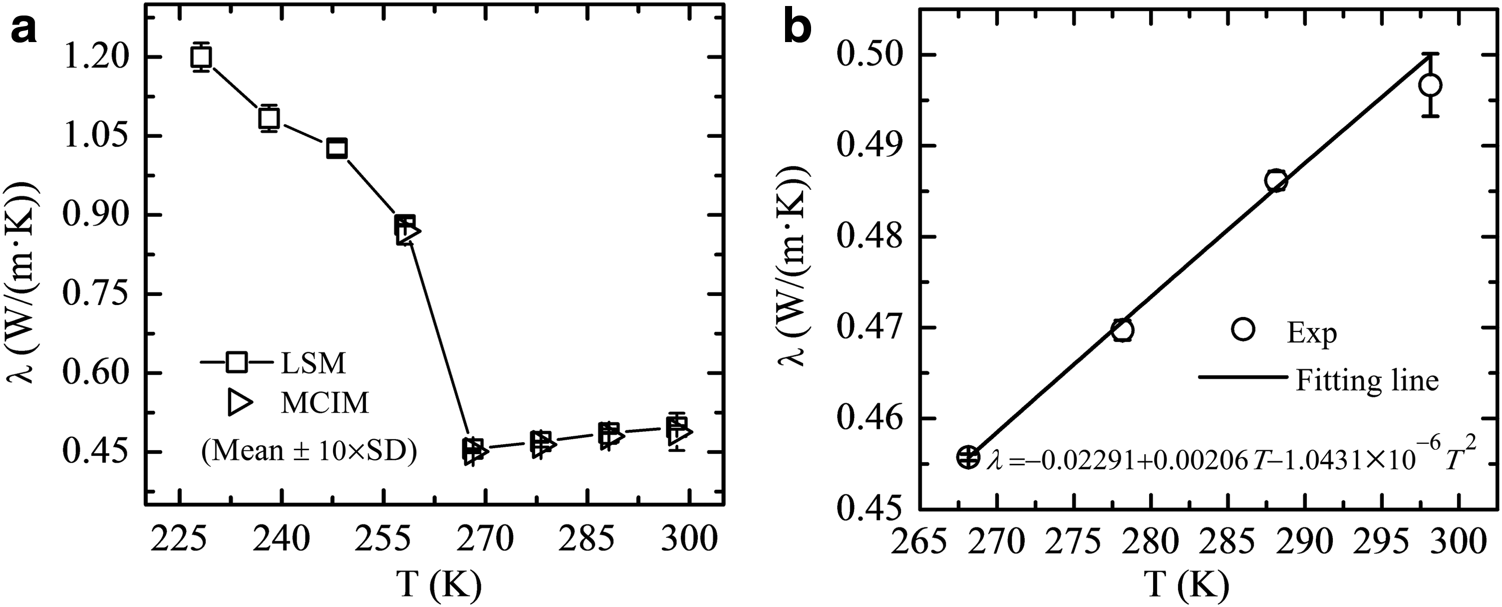
Figures 5 and 6 demonstrate the typical thermal conductivity profiles of M22 and VSED solutions, respectively. The results obtained for thermal conductivity of the two solutions (M22 and VSED) using the LSM and the MCIM are shown in Figures 5a and 6a, and the fitting curves are shown in Figures 5b and 6b using the LSM, while taking the data before phase transition, respectively.

FIG. 5.

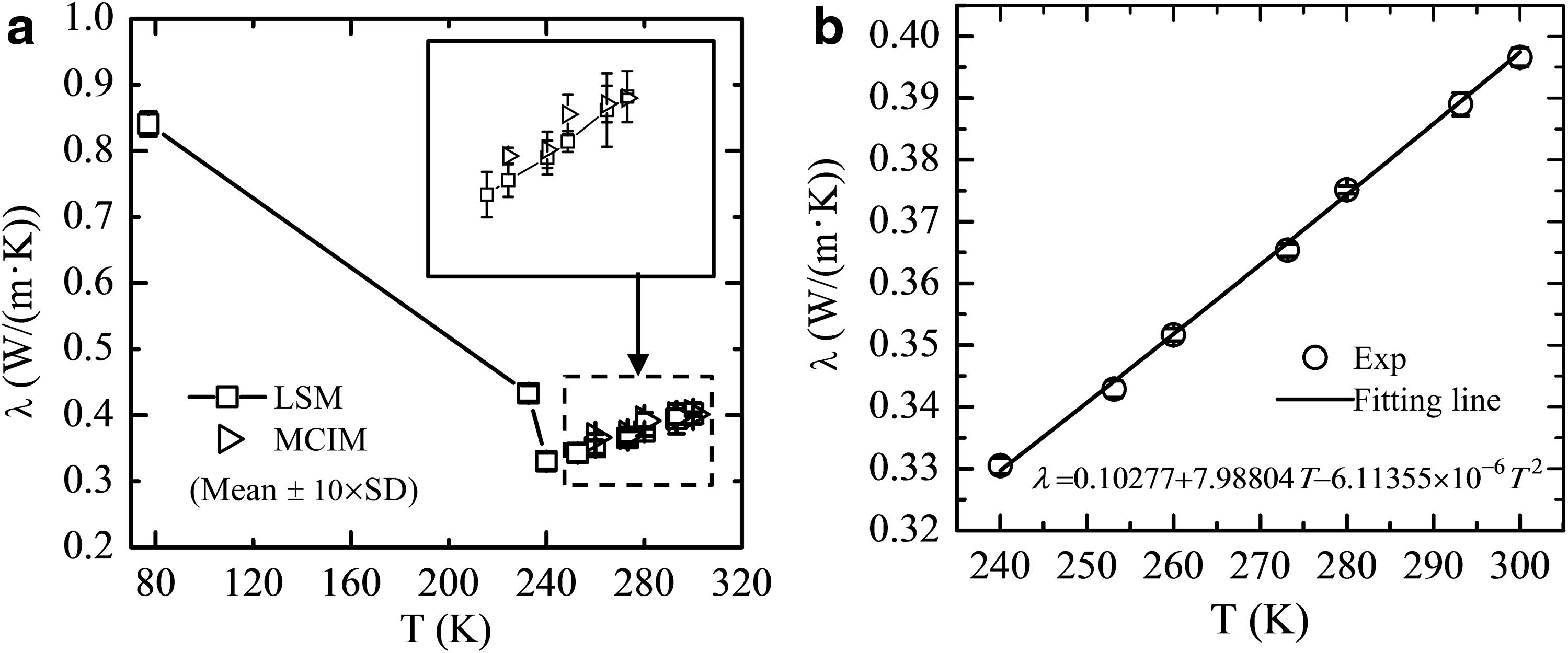
Typical thermal conductivity profiles of M22 solution. (a) The outcomes for both methods namely the LSM and the MCIM and (b) the fitting curve with LSM while taking the data before phase transition.

FIG. 6.

Typical thermal conductivity profiles of VSED solution. (a) The outcomes for both methods namely the LSM and the MCIM and (b) the fitting curve with LSM while taking the data before phase transition. VSED, vitrification solution containing ethylene glycol and dimethyl sulfoxide.

From the experimental results of the M22 and VSED solutions, we found that the phase transition temperatures of the two cryopreservation solutions are different, whereas the quadratic fitting results of thermal conductivity of the two solutions are similar before the phase transition temperature. The differences in thermal conductivity and phase transition temperature between the two cryopreservation solutions were attributed to their compositions being different.

It was found that there was an obvious difference between the MCIM and the LSM during the processing of data for obtaining thermal conductivities. The MCIM is more accurate than the LSM in some cases, although there exist some limitations of MCIM in determining the calibration constants over the entire temperature range. The LSM is more effective for the measurement of the thermal conductivities for the solids in a wide temperature range, while for liquids only the datasets excluding the effect of the convection (caused by temperature rise) can be used.

Conclusions

In this work, the thermal conductivities of M22 and VSED solutions over the wide temperature range of 77 K–300 K were determined using a self-made microscaled hot probe. Due to the fact that these parameters are not well known for the low temperatures involved in vitreous cryopreservation, while they are indispensable for a theoretical model based optimization of the vitrification processes, this study provides an invaluable addition to the published data.

Footnotes

Acknowledgment

This work was partially supported by the National Natural Science Foundation of China (Nos. 51276179, 51476160, and 51528601).

Author Disclosure Statement

No conflicting financial interests exist.

References

Asghar

, et al. Preserving human cells for regenerative, reproductive, and transfusion medicine. Biotechnol J, 2014; 9:895–903.

Huang

, et al. Alginate hydrogel microencapsulation inhibits devitrification and enables large-volume low-CPA cell vitrification. Adv Funct Mater, 2015; 25:6939–6850.

Mazur

. Kinetics of water loss from cells at subzero temperatures and likelihood of intracellular freezing. J Gen Physiol, 1963; 47:347–369.

Mazur

. Freezing of living cells—mechanisms and implications. Am J Physiol, 1984; 247:C125–C142.

Kasai

. Cryopreservation of mammalian embryos. Mol Biotechnol, 1997; 7:173–179.

Liu

, Phy

, Yeomans

. Theoretic considerations regarding slow cooling and vitrification during cryopreservation. Theriogenology, 2012; 78:1641–1652.

Davidson

, et al. Toxicity minimized cryoprotectant addition and removal procedures for adherent endothelial cells. PLoS One, 2015; 10:e0142828.

Fahy

, MacFarlane

, Angell

, Meryman

. Vitrification as an approach to cryopreservation. Cryobiology, 1984; 21:407–426.

Lucena

, Bernal

, Lucena

, Rojas

, Moran

, Lucena

. Successful ongoing pregnancies after vitrification of oocytes. Fertil Steril, 2006; 85:108–111.

10.

Leibo

, Pool

. The principal variables of cryopreservation: Solutions, temperatures, and rate changes. Fertil Steril, 2011; 96:269–276.

11.

Desrosiers

, Légaré

, Leclerc

, Sullivan

. Membranous and structural damage that occur during cryopreservation of human sperm may be time-related events. Fertil Steril, 2006; 85:1744–1752.

12.

Chen

, Yang

. Slow freezing or vitrification of oocytes: Their effects on survival and meiotic spindles, and the time schedule for clinical practice. Taiwan J Obstet Gynecol, 2009; 48:15.

13.

Fahy

, et al. Vitrification as an approach to cryopreservation. Cryobiology, 1984; 21:407–426.

14.

Jacobsen

, Pegg

. Cryopreservation of organs: A review. Cryobiology, 1984; 21:377–384.

15.

Meryman

. Cryopreservation of living cells: Principles and practice. Transfusion, 2007; 47:935–945.

16.

Hubel

. Parameters of cell freezing: Implications for the cryopreservation of stem cells. Transfus Med Rev, 1997; 11:224.

17.

Karlsson

JOM

, Toner

. Cryopreservation. In Lanza

, Vacanti

(eds). Principles of Tissue Engineering. San Diego, Academic Press. 2000; 2:293–307.

18.

Pegg

. Principles of cryopreservation. In: Day

, Stacey

(eds). Cryopreservation and Freeze-Drying Protocols. Totowa, NJ: Humana Press. 2007; 368:39–57.

19.

Almansoori

, et al. Cryoprotective agent toxicity interactions in human articular chondrocytes. Cryobiology, 2012; 64:185–191.

20.

Rall

, Fahy

. Ice-free cryopreservation of mouse embryos at −196 degrees C by vitrification. Nature, 1985; 313:573–575.

21.

Guan

, Gong

. Recent advances in cryopreservation of cells and tissues by vitrification. Int J of Biomed Eng, 2004; 27:252–256.

22.

Song

, et al. Vitreous cryopreservation maintains the function of vascular grafts. Nat Biotechnol, 2000; 18:296.

23.

Rich

, Armitage

. The potential of an equimolar combination of propane-1,2-diol and glycerol as a vitrification solution for corneas. Cryobiology, 1991; 28:314–326.

24.

Baicu

, et al. Cryopreservation of carotid artery segments via vitrification subject to marginal thermal conditions: Correlation of freezing visualization with functional recovery. Cryobiology, 2008; 57:1–8.

25.

Fahy

, et al. Cryopreservation of organs by vitrification: Perspectives and recent advances. Cryobiology, 2004; 48:157.

26.

Nagasaka

, Nagashima

. Absolute measurement of the thermal conductivity of electrically conducting liquids by the transient hot-wire method. J Phys E Sci Instrum, 1981; 14:1435.

27.

Ramires

MLV

, et al. Reference data for the thermal conductivity of saturated liquid toluene over a wide range of temperatures. J Phys Chem Ref Data, 2000; 29:133–139.

28.

Nagasaka

, Nagashima

. Simultaneous measurement of the thermal conductivity and the thermal diffusivity of liquids by the transient hot-wire method. Rev Sci Instrum, 1981; 52:229–232.

29.

Liang

, et al. A convenient method of measuring the thermal conductivity of biological tissue. Phys Med Biol, 1991; 36:1599.

30.

Cheng

, Jiang

, Liang

. A tiny heat probe for measuring the thermal conductivities of non-rigid materials. Meas Sci Technol, 1994; 5:1339.

31.

Xie

, Cheng

. A fine needle probe for determining the thermal conductivity of penetrable materials. Meas Sci Technol, 2001; 12:58.

32.

Zhang

, Zhao

, Ye

, et al. An improved hot probe technique for measurement of thermal conductivity of liquids. Mea Sci Technol, 2005; 16:1430–1435.

33.

Carslaw

, Jaeger

. Conduction of heat in solids, second edition. J Eng Mater Technol Trans ASME. 1986; 108:378.

34.

Cheng

, Zhang

, Zhao

. A new method of thermal probe for thermal conductivities measurement based on Monte Carlo inversion. J Univ Sci Technol China, 2008; 38:414–418.

35.

Ramires

MLV

, et al. Standard reference data for the thermal conductivity of water. J Phys Chem Ref Data, 1995; 24:1377–1381.

36.

Zhang

. Study on a tiny probe for determining thermal conductivity of biomaterials in low temperature. Yi Qi Yi Biao Xue Bao/Chin J Sci Instrum, 2004; 25:53–56.

37.

Zhou

, et al. Thermal conductivity of DMSO + C2H5OH, DMSO + H2O, and DMSO + C2H5OH + H2O mixtures at T = (278.15 to 338.15) K. J Chem Eng Data, 2013; 58:663–670.