Enhancing Breast Cancer Detection: A Machine Learning Approach Using Multielectrode Bioimpedance

Abstract

Background:

Early detection of cancerous tumors is a critical factor in improving treatment outcomes. To address this need, this study explores a simple, effective, and cost-efficient method for early cancer detection by measuring the bioimpedance of living tissues. Bioimpedance-based methods hold significant promise for the early detection of cancerous tumors.

Materials and Methods:

The study begins by simulating the impedance behavior of the human breast under two conditions: healthy and containing cancerous tumors. The Cole–Cole model is used to simulate the dielectric properties of both breast and tumor tissues using finite element modeling. In the measurement phase, eight electrodes are evenly distributed around the breast model to ensure comprehensive data collection. Subsequently, a dataset is prepared encompassing three breast sizes (60, 70, and 80 mm) in both the healthy and tumor-afflicted states, with tumor sizes of 5, 8, and 10 mm radius. This dataset is utilized to develop machine learning models, including support vector machines (SVM), convolutional neural networks (CNN), and random forest (RF), for breast cancer detection.

Results:

The results of this study demonstrate the practicality of integrating machine learning techniques with multielectrode bioimpedance measurements to achieve precise and automated breast cancer detection. Notably, the RF model outperformed both SVM and CNN in terms of cancer detection accuracy.

Conclusions:

This study underscores the potential of bioimpedance-based methods, coupled with machine learning algorithms, for early cancer detection. The findings suggest that RF models hold promise for accurate and automated breast cancer detection, offering a valuable tool for improving patient outcomes.

Introduction

Cancer is one of the leading causes of death globally. Worldwide, an estimated 19.3 million new cancer cases (18.1 million excluding nonmelanoma skin cancer) and almost 10.0 million cancer deaths (9.9 million excluding nonmelanoma skin cancer) occurred in 2020. Female breast cancer has surpassed lung cancer as the most commonly diagnosed cancer, with an estimated 2.3 million new cases (11.7%), followed by lung (11.4%), colorectal (10.0%), prostate (7.3%), and stomach (5.6%) cancers.¹

Early detection plays a pivotal role in managing breast cancer. Early detection involves identifying breast cancer before symptoms appear, and it encompasses methods such as breast self-exams, clinical breast exams, and mammograms. Studies, including one by Allemani et al.,² have highlighted a strong correlation between early detection and higher survival rates. For instance, localized breast cancer cases exhibit a five-year relative survival rate of 92%, underscoring the importance of detecting the disease at an early stage.

Detecting breast cancer early empowers healthcare providers to consider less aggressive treatment options. Patients may benefit from treatments such as lumpectomy (partial removal of breast tissue) instead of mastectomy (complete breast removal) or hormone therapy instead of chemotherapy. Cold et al.’s³ research discusses the potential for less extensive surgeries and milder treatment regimens when breast cancer is diagnosed early. Early detection allows for the preservation of breast tissue, which can lead to improved cosmetic outcomes and a better quality of life for survivors. Research by Waljee et al.⁴ emphasizes the significance of considering patients’ quality of life in breast cancer diagnosis and treatment decisions.

Late-stage breast cancer carries a substantial economic burden because of higher treatment costs and reduced productivity. Early detection can significantly reduce this economic impact. In Yabroff et al.,⁵ a study provides valuable insights into the economic consequences of late-stage breast cancer diagnosis, highlighting the potential for significant economic benefits associated with early detection.

Enhancing the early detection of breast cancer is pivotal in elevating survival rates, traditionally relying on mammography as the primary screening method. Mammography is a specialized radiographical method used to examine breast tissue, utilizing a dedicated X-ray apparatus tailored exclusively for breast imaging purposes. Its primary application lies in the screening, detection, and diagnosis of breast cancer. In the course of a mammogram, the breast is gently pressed between two plates to achieve uniform tissue thickness, facilitating the acquisition of precise X-ray images capable of identifying anomalies like tumors.⁶

Nevertheless, mammography grapples with substantial drawbacks, encompassing reduced sensitivity in dense breast tissue, elevated rates of false positives, and radiation exposure concerns. In recent times, significant strides have been made in the realm of breast cancer detection methods with the specific goal of mitigating these limitations.⁷

Breast magnetic resonance imaging (MRI) uses radiofrequency pulses to stimulate hydrogen nuclei contained within water molecules in the body. These stimulated nuclei emit signals, which are captured by a receiver coil positioned around the breast. Subsequently, a computer processes these signals to produce cross-sectional images of the breast. Typically, an intravenous injection of a contrast agent, such as gadolinium, is administered to heighten the signal distinctions between normal and abnormal tissues.⁸ Breast MRI is more sensitive than mammography, especially in dense breast tissue, but lower specificity leads to more false positives and higher costs.⁹

During ultrasound screening, a portable transducer is applied to the breast, systematically moved to capture images from various angles. The transducer emits sound waves that interact with breast tissue and are then captured by the same instrument. These reflected waves are transformed into electrical signals, which a computer interprets to produce detailed breast tissue images.¹⁰ Ultrasound screening markedly augmented the detection of cancers among high-risk women; however, it also yielded a substantial number of false-positive results.¹¹

Molecular breast imaging (MBI) capitalizes on the higher metabolic activity of breast cancer cells compared with normal tissue. It does so by using 99m Tc-sestamibi, a radiotracer that is absorbed by the mitochondria inside cells. Subsequently, gamma rays emitted by the radiotracer are captured by a gamma camera system, generating visual representations of the breast tissue.¹² MBI shows promise as a supplementary screening technology for women with dense breasts, yet it is worth noting that MBI involves a higher radiation dose compared with mammography and exhibits lower specificity.¹³

Bioimpedance for cancer detection

Bioimpedance, also known as bioelectrical impedance, characterizes the electrical properties of biological tissues, specifically their ability to impede the flow of electric current. It is a measure of how biological tissues resist the passage of electrical signals and can be quantified by analyzing the response to an electrical excitation, typically by calculating the ratio of voltage to current.¹⁴

Biological tissues consist of living cells organized in a three-dimensional structure. The cellular membrane takes on a bilayer lipid structure, rendering it highly capacitive. These membranes also contain channels that selectively permit the passage of molecules. Simultaneously, the intracellular and extracellular media in living cells contain numerous ions, which confer conductive properties to these tissues. Consequently, the impedance of biological tissues encompasses both capacitance and resistance. Variations in bioimpedance depend on several factors, including tissue composition, anatomical characteristics, and the frequency of the applied electrical signal (excitation).^15,16

In the context of measuring the impedance of living tissues, two prominent methods are used: the two-electrode and four-electrode methods. The former utilizes two electrodes for both current injection and voltage measurement, whereas the latter involves two pairs of electrodes, with one pair for current injection and the other for voltage measurement. Impedance is calculated by dividing the voltage by the current.

Studies have shown that alterations in the electrical properties of biological tissues, such as changes in conductivity and permittivity, lead to shifts in tissue impedance. These changes can result from variations in tissue composition, health status, or the frequency of electrical excitation. Researchers have harnessed these properties in various applications.¹⁷

In the case of tongue cancer, studies conducted at discrete frequencies, such as 20 and 50 kHz, have uncovered discernible disparities in impedance between patients afflicted by tongue cancer and their healthy counterparts, shedding light on the diagnostic potential of bioimpedance in this context.¹⁸

Similarly, when addressing liver cancer detection, impedance measurements within the frequency range of 10–200 kHz have emerged as a powerful diagnostic tool. These measurements have revealed notable differences in phase between healthy liver tissues and cancerous tumors, offering promising prospects for early diagnosis and intervention.¹⁹

Turning our attention to skin cancer, bioimpedance spectroscopy has emerged as a valuable asset in the clinical setting. This technology aids healthcare practitioners in conducting examinations and identifying potential cases of non-melanoma skin cancer, contributing to early intervention and improved patient outcomes.²⁰ Moreover, several research endeavors have explored the synergy between bioimpedance spectroscopy and advanced classification algorithms. This collaboration has demonstrated a remarkable ability to discriminate between malignant and benign skin lesions, further enhancing the diagnostic potential of bioimpedance in skin cancer assessment.^21,22

One pivotal criterion for distinguishing skin cancer from benign growths involves the relationship between lesion impedance and reference skin impedance. Multifrequency bioimpedance measurements have played a pivotal role in this regard, offering promising results in the detection of skin cancer and its differentiation from other benign conditions.²³

The advantages of using bioimpedance spectroscopy in skin cancer detection are multifaceted. It exhibits high sensitivity, aids in informed decisions regarding biopsy excisions, possesses the capability to detect both melanoma and non-melanoma skin cancer, and facilitates the longitudinal monitoring of melanocytic lesions. This ongoing monitoring, made possible through bioimpedance, has significant implications for the early detection of melanoma, potentially leading to more successful treatment outcomes.²⁴

In the context of breast cancer detection, bioimpedance has demonstrated its diagnostic potential across a spectrum of frequencies, providing insights into impedance differences between benign and cancerous breast tissues. Notably, within the frequency range of 100 Hz–2 MHz, distinct impedance behaviors have been observed, with a notable differentiation occurring at 200 kHz.²⁵ In addition, a novel approach involves comparing impedance values between the right and left breasts at a low frequency of 1 kHz, enabling the identification of malignant tumors. Significant impedance disparities in this comparison signal the necessity for further medical evaluation, highlighting the sensitivity of bioimpedance in breast cancer diagnosis.²⁶ Moreover, bioimpedance measurements offer the ability to differentiate between breast cancer and benign tumors through the computation of indicators related to the Cole–Cole parameters, offering a comprehensive assessment tool for clinicians in distinguishing between these conditions.²⁷ A significant stride in the application of bioimpedance in breast cancer care lies in its role in identifying lymphedema, a condition often associated with breast cancer patients. In a comprehensive analysis encompassing 14 distinct research investigations, bioimpedance spectroscopy was harnessed to detect lymphedema in its early stages, well before clinical symptoms became apparent. The results were compelling, demonstrating exceptional sensitivity and specificity in identifying lymphedema.²⁸ The potential of bioimpedance spectroscopy extends beyond diagnosis. It offers the early identification of lymphedema, enabling prompt intervention to halt its progression. Moreover, it proves beneficial in monitoring the responsiveness to lymphedema treatments and evaluating the effectiveness of diverse therapeutic approaches. However, it is essential to acknowledge the challenges associated with bioimpedance spectroscopy, including the need for standardized protocols, calibration, and stringent quality control measures. Variables such as temperature, hydration levels, and electrode placement can impact measurement accuracy and should be carefully considered in its application.²⁹

Materials and Methods

In this section, we will explore an elucidation of the dielectric properties of biological tissues. Furthermore, a detailed exploration of mathematical models, including the Cole−Cole and Debye models, will be presented. In addition, the section will showcase the benefits of various machine learning algorithms by highlighting promising results achieved in this domain.

Dielectric properties of biological tissues

The dielectric properties of living tissues are affected by the composition of these tissues which is affected by the health of the tissues. On the other hand, these properties are also affected by the frequency of electrical excitation applied to the living tissues.³⁰ Owing to the important applications, especially in the field of medicine, many studies have focused on measuring and modeling the behavior of electrical properties of different types of biological tissues in different frequency ranges.

Determination of the electrical properties of different breast tissue samples, which includes three classes: healthy, malignant, and benign tissues in the range from 1 to 20 GHz, where it was clear that there is a difference between the values of electrical properties of healthy tissues and cancerous tissues.³¹

The estimation of dielectric properties of healthy and malignant human skin was the purpose of many studies, in the frequency range from 20 to 100 GHz,³² in the frequency range from 1 to 100 MHz³³ where it was found that different layers of human skin showed different values of dielectric properties.

The characterization of human and porcine liver tissue in vivo and ex vivo in three states: healthy, malignant, and cirrhotic over a wide frequency range of 0.5–20 GHz, it was found a significant difference between the ex vivo dielectric properties of healthy and malignant tissues, as well as a difference in the electrical properties of healthy tissues between ex vivo and in vivo at certain frequencies.³⁴

Through a study that included 20 types of tissues, the values of dielectric properties of these tissues were determined in a wide frequency range extending from 10 Hz to 20 GHz, where the effect of frequency on these dielectric properties is cleared.³⁵

Dielectric properties of biological tissues are shown to be affected by frequency through three levels of dispersion: α, β, and γ as shown in Figure 1. The α−dispersion occurs at low frequencies and is mainly affected by the ionic atmosphere surrounding the cells (low frequencies, i.e., 10 Hz–10 kHz), the β−dispersion describes structure relaxation (10 kHz–10 MHz), and the γ−dispersion is known as the relaxation of water molecules (at high frequencies [0.1100 GHz]).^36–38

FIG. 1.

Dispersion regions, idealized.³⁸

Mathematical models of dielectric properties of biological tissues

The possibility of simulating the interaction between biological tissues and electromagnetic fields represents a starting point for many applications, especially in the medical field. Hence, the presence of models that characterize the dielectric properties of biological tissues is essential. The Debye model is giving complex relative permittivity in term of frequency and a set of parameters:^39–42 $ϵ^{*} (ω) = ϵ' (ω) - j ϵ ″ (ω)$ (1) $ϵ^{*} (w) = ϵ_{\infty} + \sum_{n = 1}^{n = N} \frac{Δ ϵ_{n}}{1 + j ω τ_{n}} - j \frac{σ_{s}}{ω ϵ_{0}}$ (2) $ϵ (ω) = ϵ' (ω)$ (3) $σ (ω) = ω ϵ_{0} ϵ ″ (ω)$ (4) where $ω$ is the angular frequency, $ϵ'$ is the frequency-dependent dielectric constant, $ϵ ″$ is the frequency-dependent dielectric loss, $ϵ_{\infty}$ is the permittivity at infinite frequency, N is the number of poles, $σ_{s}$ is the static conductivity, $ϵ_{0}$ is the free space permittivity, $Δ ϵ_{n}$ is the magnitude of the dispersion, and $τ_{n}$ is the relaxation time constant.

For second-order Debye model: $ϵ^{*} (ω) = ϵ_{\infty} + \frac{Δ ϵ_{1}}{1 + j ω τ_{1}} + \frac{Δ ϵ_{2}}{1 + j ω τ_{2}} - j \frac{σ_{s}}{ω ϵ_{0}}$ (5) $Δ ϵ_{1} = ϵ_{s} - ϵ_{2}$ (6) $Δ ϵ_{2} = ϵ_{2} - ϵ_{\infty}$ (7) where $ϵ_{s}$ and $ϵ_{\infty}$ are the low- and high-frequency constraints of the dielectric constant, respectively, and $ϵ_{2}$ is the intermediate dielectric constant for the description of the transitional state between the two relaxation processes the double Debye model has been used to describe the dielectric properties of living tissues as the skin.⁴³ A single relaxation Debye model was used within finite difference time-domain (FDTD) in order to simulate the dielectric properties of healthy and malignant skin tissues in a range from 20 to 100 GHz, where it was found that there is agreement between the obtained results and the existing experimental data.³² A double Debye model of healthy skin and basal cell carcinoma was presented in,⁴⁴ where it was confirmed the striking potential of using the parameters of double Debye model to detect skin tumor.

A single Debye dispersion model was used with magnetic resonance images (MRIs) to develop a realistic numerical model of the breast,^45–47 the same technique was used to estimate the spatially averaged dielectric properties of breast tissue.⁴⁸ Parameters for one pole and two poles Debye model for healthy and malignant breast tissues was presented in the range from 0.5 to 20 GHz.⁴⁰ The frequency dependence of the breast tissue relative permittivity and the conductivity were modeled using a single pole Debye model for microwave imaging via space-time early breast cancer detection technique.⁴⁹

By deriving fourth-order Debye model for each tissue of the head in the range from 0.1 to 3 GHz, a three-dimensional FDTD model of the head was formed that can be used to study the effect of the electromagnetic field on the head.⁵⁰

Using the same approach as Debye model, the Cole–Cole model (first presented by Cole and Cole⁵¹) describes the dispersion and absorption of a large number of liquids and dielectrics in a wide frequency range The Cole–Cole expression. Each dispersion region may become broader by various contributions because of the complexity of biological material’s structure and composition; this is why it was added a distribution parameter α with a value between 0 and 1 that describes the dispersion’s broadening. The general equation of Cole–Cole model is given in (8). $ϵ^{*} (ω) = ϵ_{\infty} + \sum_{n = 1}^{n = N} \frac{Δ ϵ_{n}}{1 + {(j ω τ_{n})}^{(1 - α_{n})}} - j \frac{σ_{s}}{ω ϵ_{0}}$ (8)

The Cole–Cole model’s order used to predict a material’s dielectric properties is defined by the considered dispersion regions.⁵²

For frequencies above a few hundred megahertz, the complex permittivity can be represented using one single pole,⁵³ as dipolar relaxation of water is the main relaxation mechanism. Then, the Cole–Cole equation can be written as: $ϵ^{*} (ω) = ϵ_{\infty} + \frac{Δ ϵ}{1 + {(j ω τ)}^{(1 - α)}} - j \frac{σ_{s}}{ω ϵ_{0}}$ (9)

The real and imaginary parts of a single dispersion Cole–Cole model are given by the equations:⁵⁴ $ϵ' = ϵ_{\infty} + \frac{(ϵ_{s} - ϵ_{\infty}) (1 + {(ω τ)}^{1 - α} Sin α \frac{π}{2})}{1 + 2 {(ω τ)}^{1 - α} Sin α \frac{π}{2} + {(ω τ)}^{2 (1 - α)}}$ (10) $ϵ ″ = \frac{((ϵ_{s} - ϵ_{\infty}) {(ω τ)}^{1 - α} C o s α \frac{π}{2})}{1 + 2 {(ω τ)}^{1 - α} S i n α \frac{π}{2} + {(ω τ)}^{2 (1 - α)}}$ (11)

The work made by Gabriel et al.⁵² for establishing a four-terms Cole–Cole model for 17 different tissue types in the frequency range from 10 Hz to 100 GHz is one of the most well-known works in this area. Another work presented by Sasaki et al.⁵⁵ has determined, through an identification algorithm, the parameters for a double Cole–Cole model of 43 types of tissues and organs in the frequency range from 1 MHz to 20 GHz.

As the Cole–Cole model allows us to overcome the complexities of experimental measurements, it was used in many studies to model the propagation of electromagnetic waves in biological tissues.^53,56 For medical applications, this model was derived for healthy and malignant breast tissue within a frequency range from 0.5 to 50 GHz, where there was a difference between the model parameters for healthy and malignant tissues.⁵⁷ In the same way, a one-pole model of normal, malignant, and benign breast tissue was derived within the frequency range from 0.5 to 20 GHz.³¹ In addition, the Cole–Cole model was used to find a relationship between changes in dielectric properties and glucose concentration in blood plasma, through which blood glucose concentration can be monitored.⁵⁸ In many other studies, this model was used to simulate near-realistic models of some human organs.^59–61

Advantages of machine learning in detecting breast cancer

Breast cancer detection has witnessed significant advancements through machine learning techniques. In a recent study, a hybrid convolutional neural network (CNN)–support vector machine (SVM) model was introduced for the automated detection of breast tumors in ultrasound images. The model exhibited impressive performance metrics, including an accuracy of 97.5%, a sensitivity of 96.0%, and a specificity of 98.3%, as demonstrated on a dataset comprising 200 ultrasound images of breast tumors. Notably, this hybrid model surpassed the individual CNN and SVM models, showcasing superior accuracy, sensitivity, and specificity in the context of breast tumor detection.⁶²

A review encompassing diverse deep learning techniques for breast cancer detection across multiple modalities, encompassing mammography, ultrasound, thermography, and MRI, was conducted. It was concluded that the CNN classifier is deemed suitable for early breast cancer detection, attaining a notable 99% accuracy when compared with alternative classifiers. Furthermore, the complexities and forthcoming directions within the field of deep learning for breast cancer detection were discussed.⁶³

An optimized SVM-based model was introduced for breast cancer prediction using the Bayesian search method to identify the optimal hyperparameters of the SVM classifier. Evaluation was conducted on two datasets, namely the Wisconsin Breast Cancer Dataset (WBCD) and Breast Cancer Coimbra Dataset (BCCD). The results indicated that an accuracy of 97.14% was attained on WBCD, while 83.33% accuracy was achieved on BCCD. These accuracies surpassed those of the SVM classifier with default hyperparameters.⁶⁴

A breast cancer contour detection model was introduced, designed for application in conventional ultrasound, elasticity, and Doppler images. The segmentation of contours was carried out using region-based level sets, followed by classification using SVM to discern between breast cancer contours and false contours. Features were extracted from level sets and through the FM method, which combines information from ultrasound, elasticity, and Doppler images. The model achieved an impressive accuracy rate of 98.5% when tested on a dataset containing 40 breast tumor images.⁶⁵

CNN method is proposed to improve breast cancer identification in whole-slide images. Using various CNN architectures and a large dataset of 275,000 50 × 50-pixel RGB image patches, the system achieves an 87% accuracy rate. This approach has the potential to reduce diagnostic errors.⁶⁶

The CNN algorithm, utilizing the Wisconsin breast cancer dataset, demonstrates impressive performance in binary classification (benign vs. malignant). The novel CNN model achieves a remarkable validation accuracy of 97.85%, outperforming both the standard CNN and LSTM models, which achieve accuracies of 94.12% and 93.50%, respectively, with different optimizers. Meanwhile, the multilayer perceptron attains an accuracy of 92.44% using the Adam optimizer.⁶⁷

An automated model for cancer detection and classification from microscopic biopsy images utilizing biologically interpretable features was proposed. The approach used the Socially Spider Optimization encryption method in conjunction with a neural network for categorizing cancerous biopsy images. The framework’s performance was assessed using accuracy, sensitivity, specificity, and Matthews Correlation Coefficient evaluations, resulting in respective values of 95.91%, 94.25%, 97.12%, and 97.68%.⁶⁸

A cost-sensitive learning approach for breast cancer classification using the random forest (RF) algorithm was proposed. The model was evaluated on the Wisconsin breast cancer dataset and achieved an accuracy of 97.51%.⁶⁹

A machine learning approach for breast cancer prediction utilized the WBCD and two classifiers, RF and Gaussian Naïve Bayes. To address the dataset imbalance, the Borderline Synthetic Minority Oversampling Technique (BSM) was applied. Results show that the combination of BSM with the RF algorithm achieved the highest recall score, ∼99.80%, whereas BSM with the Gaussian Naïve Bayes classifier resulted in the lowest recall score, at 78.20%.⁷⁰

Simulations

The impedance values for tissues with tumors exhibit a consistent pattern of being lower than those for healthy tissue, indicating that the presence of a tumor significantly influences the electrical properties of the tissue. Furthermore, as the tumor size increases, the impedance values decrease more substantially, underscoring the greater impact of larger tumors on tissue impedance.

In the case of human breast tissue, as depicted in Figure 2, a similar trend is observed. With increasing frequency, the difference in impedance between healthy breast tissue and breast tissue with tumors diminishes. For instance, at 20 kHz, the impedance difference between healthy breast tissue and breast tissue with a 20 mm tumor is 294.6 Ω, whereas at 100 MHz, the difference reduces to 82.15 Ω. Similarly, at 20 kHz, the impedance difference between healthy breast tissue and breast tissue with a 10 mm tumor is 41.5 Ω, whereas for breast tissue with a 20 mm tumor, the difference significantly increases to 294.6 Ω. This observation highlights that larger tumors result in more pronounced differences in impedance compared with smaller tumors.

FIG. 2.

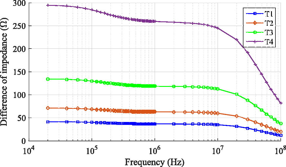
Difference of impedance between normal human breast and human breast containing a tumor in the frequency range from 20 kHz to 100 MHz, with tumor radius: T1 = 10 mm, T2 = 12 mm, T3 = 15 mm, and T4 = 20 mm.

In our study, we leverage this characteristic to effectively distinguish between healthy breast tissue and breast tissue containing tumors. Based on these findings, we have chosen a minimum frequency of 20 kHz for bioimpedance measurements.

In the initial step of our simulation, we developed a breast model representing it as a half-sphere as shown in Figure 3. To accurately capture the dielectric properties of breast tissue, we incorporated the Cole–Cole model. Similarly, within this breast model, we represented the tumor as a sphere, and its dielectric properties were also characterized using the Cole–Cole model. The dielectric properties of the tissues are modeled using Cole–Cole parameters as shown in Table 1 for human breast. For the purpose of electrical impedance measurements, we positioned a set of eight negative electrodes evenly distributed around the base of the breast model. In addition, a positive electrode was placed on the top of the breast model.

FIG. 3.

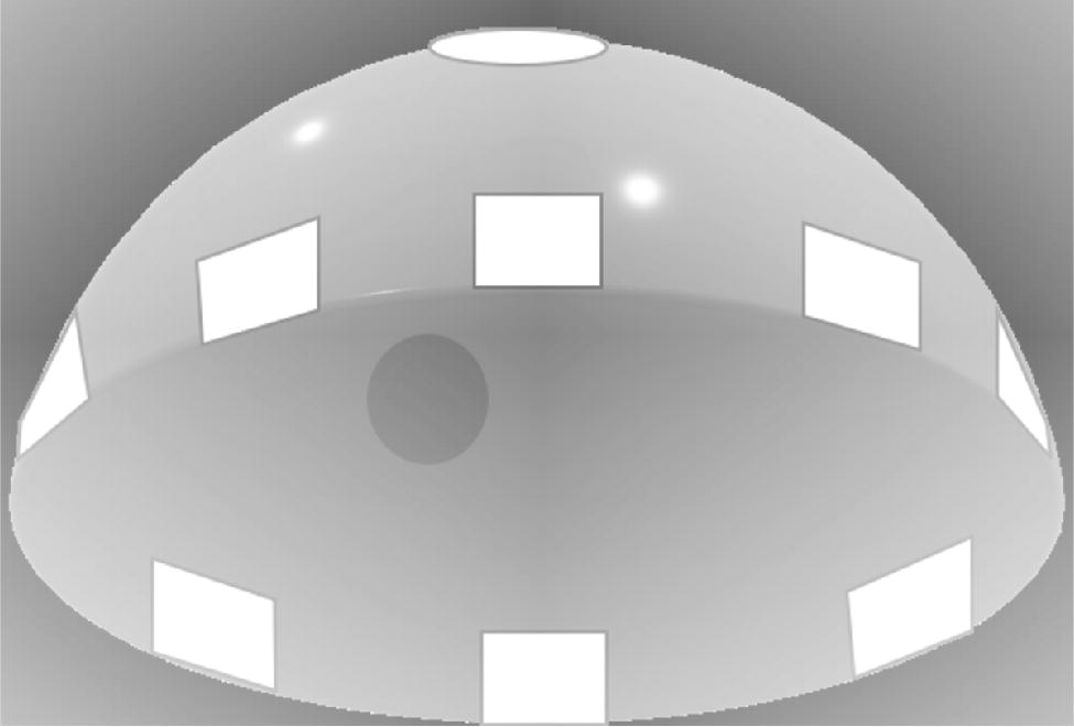
3D breast model containing a tumor and surrounded by 8 negative electrodes, with the positive electrode positioned on top.

Table 1.

Cole–Cole Parameters for Normal Breast Tissue and Tumor in the Frequency Range from 20 kHz to 100 MHz⁷¹

	ϵ_∞	ϵ _s	α	τ	σ _s
Normal	10	288	0.1	9.83E-07	0.0161
Tumor	50	6090	0.326	6.33E-07	0.22

In this simulation, we incorporated three distinct breast sizes, each characterized by a radius of 60, 70, and 80 mm, respectively. Within each of these breast sizes, tumors of varying sizes, with radius of 5, 8, and 10 mm, were introduced.

To comprehensively assess the impact of these parameters, we conducted 200 bioimpedance measurements for each combination of breast size and tumor size. During each measurement, we used the Latin hypercube sampling (LHS) algorithm to calculate the coordinates for the tumor’s position within the breast model. This allowed us to capture the dynamic impedance behavior associated with different tumor positions.

In addition to the tumor-focused measurements, we performed 100 bioimpedance measurements for healthy breasts without tumors in each breast size category. For each measurement, we utilized the LHS algorithm to determine the coordinates for slight perturbations in the position of the positive electrode. In total, for each breast size, we conducted 4,800 measurements with tumors, considering 200 tumor positions, 3 tumor sizes, and 8 electrodes. In addition, we performed 800 measurements without tumors, accounting for 100 different positions of the positive electrode and 8 electrodes in total. By adopting this comprehensive approach, we were able to thoroughly explore the bioimpedance characteristics of breasts containing tumors of varying sizes and positions, while also establishing a baseline for healthy breast tissue impedance.

Following the preparation of the dataset, we proceeded with the classification process, using three distinct machine learning methods: SVM, RF, and CNN. The classification process is divided into two distinct parts. In the first part, individual classifications are performed for each breast size, considering all tumor sizes within each category. Subsequently, in the second part, a global classification is conducted, encompassing all breast sizes and tumor sizes, as illustrated in the following algorithm steps:

Initialization

Initialize arrays, variables, and data structures.

Create arrays for storing evaluation metrics.

Data Preparation

Define breast size categories.

For each breast size category:

Augment the healthy data to match the tumor data.

Combine the data and create corresponding labels.

Normalize the impedance values using z-score normalization.

Individual Machine Learning Models

For each breast size category:

Perform 5-fold cross-validation.

Train a machine learning model.

Evaluate the model’s performance.

Save the trained model for the current breast size.

Global Machine Learning Model (a)

Initialize arrays for storing metrics of the global model.

(b)

Perform 5-fold cross-validation for the combined dataset.

(c)

Train a global machine learning model.

(d)

Evaluate the global model’s performance.

Next, the results of our classification experiments using various machine learning techniques will be discussed.

Results

In this section, we will present the outcomes obtained from using various machine learning algorithms for breast cancer detection.

SVM model performance

The outcomes obtained from using SVM algorithm for breast cancer detection include the following:

Breast Size 60 mm: The SVM model for breast tissue samples of 60 mm achieves an average accuracy of 84.00% with a relatively low standard deviation of 2.36%. This indicates reasonable performance in classifying breast tissue samples of this size. Sensitivity is high at 95.17% with a low standard deviation of 2.25%, suggesting the model’s effectiveness in detecting tumors. However, specificity is relatively low at 50.50% with a higher standard deviation of 7.79%, indicating some challenges in correctly classifying healthy tissue samples. The F1 score is 0.66 with a small standard deviation of 0.07, indicating a balanced performance between precision and recall.

Breast Size 70 mm: For breast tissue samples of 70 mm, the SVM model achieves a high accuracy of 97.50% with a low standard deviation of 0.99%, demonstrating excellent overall performance. Sensitivity is also high at 98.50% with a low standard deviation of 1.60%, indicating effective tumor detection. Specificity is 94.50% with a standard deviation of 4.11%, suggesting good performance in correctly classifying healthy tissue samples. The F1 score is 0.96 with a small standard deviation of 0.02, signifying a very balanced performance between precision and recall.

Breast Size 80 mm: The SVM model for breast tissue samples of 80 mm achieves an extremely high accuracy of 99.25% with a very low standard deviation of 0.68%, indicating nearly perfect performance. Sensitivity is also extremely high at 99.67% with a low standard deviation of 0.46%, effectively identifying tumors. Specificity is 98.00% with a standard deviation of 2.09%, suggesting excellent performance in correctly classifying healthy tissue samples. The F1 score is 0.99 with a small standard deviation of 0.01, demonstrating an outstanding balance between precision and recall.

Global SVM Model: The global SVM model achieves an accuracy of 90.50% with a moderate standard deviation of 1.07%, indicating good overall performance across different breast sizes. Sensitivity is 93.72% with a standard deviation of 1.40%, effectively identifying tumors globally. Specificity is 80.83% with a standard deviation of 4.56%, indicating moderate performance in correctly classifying healthy tissue samples. The F1 score is 0.87 with a small standard deviation of 0.02, signifying a reasonably balanced performance between precision and recall on the global dataset. These results are summarized in Table 2.

Table 2.

Performance Metrics for Breast Size SVM Models and Global SVM Model

Performance metric	Mean	Standard deviation
Breast size: 60 mm
Accuracy	84.00%	±2.36%
Sensitivity	95.17%	±2.25%
Specificity	50.50%	±7.79%
F1 score	0.66	±0.07
Breast size: 70 mm
Accuracy	97.50%	±0.99%
Sensitivity	98.50%	±1.60%
Specificity	94.50%	±4.11%
F1 score	0.96	±0.02
Breast size: 80 mm
Accuracy	99.25%	±0.68%
Sensitivity	99.67%	±0.46%
Specificity	98.00%	±2.09%
F1 score	0.99	±0.01
Global SVM model
Accuracy	90.50%	±1.07%
Sensitivity	93.72%	±1.40%
Specificity	80.83%	±4.56%
F1 score	0.87	±0.02

SVM, support vector machine.

CNN model performance

The outcomes obtained from using CNN algorithm for breast cancer detection:

Breast Size 60 mm (CNN): The CNN model for breast tissue samples of 60 mm achieves an average accuracy of 95.75% with a standard deviation of 8.81%. This suggests that the CNN model performs well in classifying breast tissue samples of this size. Sensitivity is 94.50% with a higher standard deviation of 12.30%, indicating effective tumor detection. Specificity is 97.00% with a standard deviation of 5.36%, demonstrating good performance in correctly classifying healthy tissue samples. The F1 score is 0.96 with a standard deviation of 0.09, indicating a balanced performance between precision and recall.

Breast Size 70 mm (CNN): For breast tissue samples of 70 mm, the CNN model achieves a very high accuracy of 99.75% with a low standard deviation of 0.37%, indicating excellent overall performance. Sensitivity is extremely high at 99.83% with a small standard deviation of 0.37%, effectively identifying tumors. Specificity is 99.67% with a slightly higher standard deviation of 0.75%, suggesting strong performance in correctly classifying healthy tissue samples. The F1 score is a perfect 1.00 with a standard deviation of 0.00, signifying an outstanding balance between precision and recall.

Breast Size 80 mm (CNN): The CNN model for breast tissue samples of 80 mm achieves an exceptional accuracy of 100.00% with no standard deviation, indicating perfect performance. Sensitivity is also perfect at 100.00% with no standard deviation, effectively identifying tumors. Specificity is also perfect at 100.00% with no standard deviation, demonstrating flawless performance in correctly classifying healthy tissue samples. The F1 score is 1.00 with no standard deviation, showcasing a perfect balance between precision and recall.

Global Neural Network (CNN): The global CNN model achieves an accuracy of 89.53% with a moderate standard deviation of 3.46%, indicating good overall performance across different breast sizes. Sensitivity is 91.50% with a standard deviation of 3.55%, effectively identifying tumors globally. Specificity is 87.56% with a standard deviation of 3.80%, indicating moderate performance in correctly classifying healthy tissue samples. The F1 score is 0.89 with a standard deviation of 0.03, signifying a reasonably balanced performance between precision and recall on the global dataset. A summary of the results can be found in Table 3.

Table 3.

Performance Metrics for Breast Size CNN Models and Global CNN Model

Performance metric	Mean	Standard deviation
Breast size: 60 mm
Accuracy	95.75%	±8.81%
Sensitivity	94.50%	±12.30%
Specificity	97.00%	±5.36%
F1 score	0.96	±0.09
Breast size: 70 mm
Accuracy	99.75%	±0.37%
Sensitivity	99.83%	±0.37%
Specificity	99.67%	±0.75%
F1 score	1.00	±0.00
Breast size: 80 mm
Accuracy	100.00%	±0.00%
Sensitivity	100.00%	±0.00%
Specificity	100.00%	±0.00%
F1 score	1.00	±0.00
Global Neural Network
Accuracy	89.53%	±3.46%
Sensitivity	91.50%	±3.55%
Specificity	87.56%	±3.80%
F1 score	0.89	±0.03

CNN, convolutional neural network.

RF model performance

For the RF technique, in contrast to the other two models used in this study, we adopted a unique approach that involved varying the number of electrodes from 2 to 8. This approach allowed us to assess the influence of the number of electrodes on the performance of the RF model. The findings are presented in Table 4.

Table 4.

Performance Metrics for Different Measurements and Breast Sizes for Random Forest Model

Number ofelectrodes	Breast size	Average accuracy	Average sensitivity	Average specificity	Average F1 score
2	60 mm	96.25% ± 1.17%	96.67% ± 1.32%	95.00% ± 3.54%	0.96 ± 0.02
2	70 mm	95.38% ± 2.05%	97.33% ± 2.31%	89.50% ± 5.70%	0.93 ± 0.03
2	80 mm	97.25% ± 0.84%	97.33% ± 1.49%	97.00% ± 2.74%	0.97 ± 0.01
3	60 mm	96.75% ± 1.73%	97.67% ± 1.81%	94.00% ± 4.18%	0.96 ± 0.02
3	70 mm	97.75% ± 1.14%	98.33% ± 1.95%	96.00% ± 2.24%	0.97 ± 0.01
3	80 mm	98.25% ± 0.52%	98.33% ± 0.59%	98.00% ± 2.74%	0.98 ± 0.01
4	60 mm	98.87% ± 1.20%	99.50% ± 0.46%	97.00% ± 4.47%	0.98 ± 0.02
4	70 mm	99.00% ± 1.37%	99.33% ± 0.91%	98.00% ± 2.74%	0.99 ± 0.02
4	80 mm	99.38% ± 0.62%	99.17% ± 0.83%	100.00% ± 0.00%	1.00 ± 0.00
5	60 mm	99.38% ± 1.08%	99.83% ± 0.37%	98.00% ± 4.47%	0.99 ± 0.02
5	70 mm	99.25% ± 0.81%	99.83% ± 0.37%	97.50% ± 3.54%	0.99 ± 0.02
5	80 mm	98.63% ± 0.81%	98.83% ± 0.95%	98.00% ± 2.74%	0.98 ± 0.01
6	60 mm	99.75% ± 0.56%	99.67% ± 0.75%	100.00% ± 0.00%	1.00 ± 0.00
6	70 mm	100.00% ± 0.00%	100.00% ± 0.00%	100.00% ± 0.00%	1.00 ± 0.00
6	80 mm	100.00% ± 0.00%	100.00% ± 0.00%	100.00% ± 0.00%	1.00 ± 0.00
7	60 mm	99.75% ± 0.34%	99.67% ± 0.46%	100.00% ± 0.00%	1.00 ± 0.00
7	70 mm	100.00% ± 0.00%	100.00% ± 0.00%	100.00% ± 0.00%	1.00 ± 0.00
7	80 mm	100.00% ± 0.00%	100.00% ± 0.00%	100.00% ± 0.00%	1.00 ± 0.00
8	60 mm	100.00% ± 0.00%	100.00% ± 0.00%	100.00% ± 0.00%	1.00 ± 0.00
8	70 mm	100.00% ± 0.00%	100.00% ± 0.00%	100.00% ± 0.00%	1.00 ± 0.00
8	80 mm	100.00% ± 0.00%	100.00% ± 0.00%	100.00% ± 0.00%	1.00 ± 0.00
2	Global RF Model	94.17% ± 1.18%	94.72% ± 1.52%	92.50% ± 4.17%	0.94 ± 0.02
3	Global RF Model	96.33% ± 1.04%	97.33% ± 1.33%	93.33% ± 1.67%	0.95 ± 0.01
4	Global RF Model	97.42% ± 0.64%	98.22% ± 0.42%	95.00% ± 3.12%	0.97 ± 0.02
5	Global RF Model	98.08% ± 0.65%	99.00% ± 0.32%	95.33% ± 2.74%	0.97 ± 0.01
6	Global RF Model	99.29% ± 0.79%	99.28% ± 0.70%	99.33% ± 1.49%	0.99 ± 0.01
7	Global RF Model	99.75% ± 0.27%	99.78% ± 0.23%	99.67% ± 0.75%	1.00 ± 0.00
8	Global RF Model	99.67% ± 0.43%	99.78% ± 0.23%	99.33% ± 1.49%	1.00 ± 0.00

RF, random forest.

Breast Size 60 mm (RF): As the number of measurements increases from 2 to 8 for each tumor position, there is a consistent improvement in the performance of the RF model for breast tissue samples of 60 mm. The average accuracy increases from 96.25% to 100.00%, indicating that the RF model becomes more accurate in classifying breast tissue samples of this size. Sensitivity, which measures the model’s ability to correctly identify tumors, also increases from 96.67% to 100.00%, indicating that the RF model becomes more effective in detecting tumors as the number of measurements increases. Specificity, which measures the model’s ability to correctly classify healthy tissue samples, also improves from 95.00% to 100.00%, indicating better performance in identifying healthy tissue. The F1 score, which balances precision and recall, consistently improves from 0.96 to 1.00, indicating a more balanced and effective classification.

Breast Size 70 mm (RF): Similar to the 60 mm breast size, as the number of measurements increases, the RF model’s performance consistently improves for breast tissue samples of 70 mm. Accuracy increases from 95.38% to 100.00%. Sensitivity increases from 97.33% to 100.00%, indicating improved tumor detection. Specificity improves from 89.50% to 100.00%, showing better identification of healthy tissue samples. The F1 score increases from 0.93 to a perfect 1.00, demonstrating a balanced performance.

Breast Size 80 mm (RF): For breast tissue samples of 80 mm, the RF model already starts with high performance and maintains it as the number of measurements increases. Accuracy remains consistently high at 97.25% to 100.00%. Sensitivity remains high at 97.33% to 100.00%, indicating strong tumor detection. Specificity remains consistently excellent at 97.00% to 100.00%, indicating accurate identification of healthy tissue. The F1 score remains high at 0.97 to 1.00, demonstrating a balanced performance.

Global RF Model (RF): In the global RF model, there is a similar trend of performance improvement with an increasing number of measurements. Accuracy increases from 94.17% to 99.75%, indicating better overall performance as more measurements are considered. Sensitivity increases from 94.72% to 99.78%, showing improved tumor detection globally. Specificity improves from 92.50% to 99.67%, indicating better identification of healthy tissue samples. The F1 score increases from 0.94 to 1.00, demonstrating a balanced and effective classification.

In summary, increasing the number of measurements (electrodes) generally leads to improved performance for both specific breast sizes and the global RF model. This improvement is observed in terms of accuracy, sensitivity, specificity, and the F1 score, indicating that more measurements provide better information for classifying breast tissue samples and detecting tumors.

Interestingly, our findings suggest the existence of a saturation point where increasing the number of measurements leads to only marginal improvements in performance. Specifically, the shift from 6 to 8 measurements for each tumor position, especially in the case of larger breast sizes, resulted in relatively minor performance gains.

This observation implies the presence of an optimal balance between the quantity of measurements and computational resources. Beyond a certain threshold, accumulating more measurements may not necessarily lead to significant enhancements in model performance. This underscores the importance of exercising prudence in weighing the efforts of data acquisition against the associated costs and computational complexities.

In the comparative analysis of the global classification models, the RF model emerges as the top performer. RF achieved an exceptional accuracy of 99.67%, the highest sensitivity of 99.78%, and specificity of 99.33%, resulting in a perfect F1 score of 1.00. In contrast, the SVM model exhibited lower accuracy (90.50%) and sensitivity (93.72%) with moderate specificity (80.83%) and an F1 score of 0.87. The CNN model also showed competitive performance with an accuracy of 89.53%, sensitivity of 91.50%, specificity of 87.56%, and an F1 score of 0.89. Thus, the RF model demonstrates superior classification capabilities, making it the preferred choice for this task.

Discussion

In this study, we investigated the performance of various machine learning models for breast cancer detection, including SVM, CNN, and RF models. The results obtained from these models demonstrate promising accuracy and sensitivity in classifying breast tissue samples of different sizes, highlighting their effectiveness in tumor detection.

The SVM model exhibited reasonable performance for breast tissue samples of 60 mm, achieving an average accuracy of 84.00% and high sensitivity (95.17%). However, specificity was relatively low at 50.50%, indicating challenges in correctly classifying healthy tissue samples. As breast tissue size increased to 70 and 80 mm, the SVM model’s accuracy improved, reaching 97.50% and 99.25%, respectively. Sensitivity increased, while specificity remained relatively stable.

The CNN model demonstrated competitive performance, with an accuracy of 89.53% and an F1 score of 0.89 for the global dataset. High sensitivity and strong specificity indicated effective tumor detection and good performance in identifying healthy tissue samples. As the breast tissue size increased, the CNN model’s accuracy improved, reaching 99.75% for both 70 mm and 80 mm sizes, with sustained high sensitivity and improved specificity.

The RF model exhibited excellent performance across different breast sizes, achieving high accuracy, sensitivity, and specificity. With an increase in the number of measurements, the RF model’s performance consistently improved, reaching perfect accuracy, sensitivity, and specificity for breast tissue samples of 60, 70, and 80 mm. This suggests that the RF model becomes more accurate and effective as more measurements are considered.

In comparing the global classification models, the RF model emerged as the top performer, achieving an exceptional accuracy of 99.67%, the highest sensitivity of 99.78%, and the highest specificity of 99.33%, resulting in a perfect F1 score of 1.00. In contrast, the SVM model exhibited lower accuracy (90.50%) and sensitivity (93.72%) with moderate specificity (80.83%) and an F1 score of 0.87. The Convolutional Neural Network model also showed competitive performance with an accuracy of 89.53%, sensitivity of 91.50%, specificity of 87.56%, and an F1 score of 0.89.

These results underscore the potential of machine learning models in breast cancer detection and emphasize the importance of selecting an appropriate model based on specific task requirements. The RF model demonstrated superior classification capabilities, making it the preferred choice for this task. However, further research is needed to investigate the impact of different model parameters, feature selection techniques, and data preprocessing methods on model performance.

Conclusion

This study has showcased the utility of bioimpedance as a powerful tool for the early detection of breast cancer. It underscores the importance of using multielectrode configurations for bioimpedance measurements, which significantly contribute to the accuracy and reliability of breast cancer detection. Moreover, this research highlights the pivotal role of machine learning techniques in enhancing the detection capabilities of breast cancer, particularly in automated and precise classification tasks.

Through a comprehensive comparison of results, it is evident that the RF machine learning model outperforms SVM and CNN in the context of breast cancer detection. RF exhibited exceptional accuracy, sensitivity, specificity, and achieved a perfect F1 score, making it the preferred choice for this vital medical application.

As a future direction, this study could be further improved by extending the analysis to include smaller tumor sizes and a more extensive dataset obtained from experimental measurements. This expansion could provide even greater insights into the effectiveness of bioimpedance-based breast cancer detection and contribute to the ongoing efforts to improve early diagnosis and treatment outcomes in breast cancer patients.

Footnotes

Acknowledgment

The authors acknowledge Ecole Militaire Polytechnique for providing the necessary resources and facilities for this research.

Authors’ Contributions

O.B.: Conceptualization, investigation, visualization, writing—original draft, and writing—reviewing and editing. Y.A.: Investigation, writing—original draft, and writing—reviewing and editing. A.Z.: Supervision, investigation, and writing—reviewing and editing.

Author Disclosure Statement

No competing financial interests exist.

Funding Information

No funding was received for this article.

References

Sung

, Ferlay

, Siegel

, et al. Global cancer statistics 2020: GLOBOCAN estimates of incidence and mortality worldwide for 36 cancers in 185 countries. CA Cancer J Clin, 2021; 71(3):209–249.

Allemani

, Matsuda

, Di Carlo

, et al. Global surveillance of trends in cancer survival 2000–14 (CONCORD-3): Analysis of individual records for 37 513 025 patients diagnosed with one of 18 cancers from 322 population-based registries in 71 countries. Lancet, 2018; 391(10125):1023–1075.

Cold

, Düring

, Ewertz

, et al. Does timing of adjuvant chemotherapy influence the prognosis after early breast cancer? Results of the Danish Breast Cancer Cooperative Group (DBCG). Br J Cancer, 2005; 93(6):627–632.

Waljee

, Rogers

, Alderman

. Decision aids and breast cancer: Do they influence choice for surgery and knowledge of treatment options? J Clin Oncol, 2007; 25(9):1067–1073.

Yabroff

, Bradley

, Mariotto

, et al. Estimates and projections of value of life lost from cancer deaths in the United States. J Natl Cancer Inst, 2008; 100(24):1755–1762.

Sardanelli

, Aase

, Álvarez

, et al. Position paper on screening for breast cancer by the European Society of Breast Imaging (EUSOBI) and 30 national breast radiology bodies from Austria, Belgium, Bosnia and Herzegovina, Bulgaria, Croatia, Czech Republic, Denmark, Estonia, Finland, France, Germany, Greece, Hungary, Iceland, Ireland, Italy, Israel, Lithuania, Moldova, The Netherlands, Norway, Poland, Portugal, Romania, Serbia, Slovakia, Spain, Sweden, Switzerland and Turkey. Eur Radiol, 2017; 27(7):2737–2743.

Jaglan

, Dass

, Duhan

. Breast cancer detection techniques: Issues and challenges. J Inst Eng India Ser B, 2019; 100(4):379–386.

Lee

, Dershaw

, Kopans

, et al. Breast cancer screening with imaging: Recommendations from the Society of Breast Imaging and the ACR on the Use of Mammography, Breast MRI, Breast Ultrasound, and Other Technologies for the Detection of Clinically Occult Breast Cancer. J Am Coll Radiol, 2010; 7(1):18–27.

Hunt

. Molecular breast imaging: A scientific review. J Breast Imaging, 2021; 3(4):416–426.

10.

Berg

, Blume

, Cormack

, et al. Combined screening with ultrasound and mammography vs mammography alone in women at elevated risk of breast cancer. JAMA, 2008; 299(18):2151–2163.

11.

Liu

, Zhan

, Sun

, et al. Comparison of BSGI, MRI, mammography, and ultrasound for the diagnosis of breast lesions and their correlations with specific molecular subtypes in Chinese women. BMC Med Imaging, 2020; 20(1):98.

12.

Rhodes

, Hruska

, Conners

, et al. Journal club: Molecular breast imaging at reduced radiation dose for supplemental screening in mammographically dense breasts. AJR Am J Roentgenol, 2015; 204(2):241–251.

13.

Iranmakani

, Mortezazadeh

, Sajadian

, et al. A review of various modalities in breast imaging: Technical aspects and clinical outcomes. Egypt J Radiol Nucl Med, 2020; 51(1):1–22.

14.

Amini

, Hisdal

, Kalvøy

. Applications of bioimpedance measurement techniques in tissue engineering. J Electr Bioimpedance, 2018; 9(1):142–158; doi: 10.2478/joeb-2018-0019

15.

Bera

. Bioelectrical impedance and the frequency dependent current conduction through biological tissues: A short review. IOP Conf Ser: Mater Sci Eng, 2018; 331:012005; doi: 10.1088/1757-899X/331/1/012005

16.

Bera

. Bioelectrical impedance methods for noninvasive health monitoring: A review. J Med Eng, 2014; 2014:381251; doi: 10.1155/2014/381251

17.

Stupin

, Kuzina

, Abelit

, et al. Bio-Impedance Spectroscopy: Basics and Applications. arXiv:200503275 [physics]; 2020.

18.

Sun

, Ching

CTS

, Cheng

, et al. The use of bioimpedance in the detection/screening of tongue cancer. Cancer Epidemiol, 2010; 34(2):207–211; doi: 10.1016/j.canep.2009.12.017

19.

Salazar-Anguiano

, Elías

, Zúñiga-García

, et al. Liver cancer analysis using bioimpedance. In: VI Latin American Congress on Biomedical Engineering CLAIB 2014, Paraná, Argentina 29, 30 & 31 October 2014. Springer; 2015. p. 17–19.

20.

Liebich

, Bruehl

, Schubert

, et al. Retrospective evaluation of the performance of the electrical impedance spectroscopy system nevisense in detecting keratinocyte cancers. Skin Research and Technology, 2021; 27(5):723–729; doi: 10.1111/srt.13007

21.

Aberg

, Geladi

, Nicander

, et al. Non-invasive and microinvasive electrical impedance spectra of skin cancer—A comparison between two techniques. Skin Res Technol, 2005; 11(4):281–286; doi: 10.1111/j.0909-725X.2005.00125.x

22.

Mohr

, Birgersson

, Berking

, et al. Electrical impedance spectroscopy as a potential adjunct diagnostic tool for cutaneous melanoma. Skin Res Technol, 2013 May;19(2):75–83; doi: 10.1111/srt.12008

23.

Aberg

, Nicander

, Hansson

, et al. Skin cancer identification using multifrequency electrical impedance—A potential screening tool. IEEE Trans Biomed Eng, 2004; 51(12):2097–2102; doi: 10.1109/TBME.2004.836523

24.

Heibel

, Hooey

, Cockerell

. A review of noninvasive techniques for skin cancer detection in dermatology. Am J Clin Dermatol, 2020; 21(4):513–524; doi: 10.1007/s40257-020-00517-z

25.

Pandya

, Kim

, Roy

, et al. Towards an automated MEMSbased characterization of benign and cancerous breast tissue using bioimpedance measurements. Sens Actuators B Chem, 2014; 199:259–268; doi: 10.1016/j.snb.2014.03.065

26.

Mansouri

, Alhadidi

, Azouz

. Breast cancer detection using low-frequency bioimpedance device. Breast Cancer: Targets Therapy, 2020; 12:109.

27.

, Wan

, Chen

, et al. Bioimpedance spectroscopy can precisely discriminate human breast carcinoma from benign tumors. Medicine, 2017; 96(4):e5970; doi: 10.1097/MD.0000000000005970

28.

Shah

, Vicini

, Arthur

. Bioimpedance spectroscopy for breast cancer related lymphedema assessment: Clinical practice guidelines. Breast J, 2016; 22(6):645–650.

29.

Forte

, Huayllani

, Boczar

, et al. Bioimpedance spectroscopy for assessment of breast cancer-related lymphedema: A systematic review. Plast Surg Nurs, 2020; 40(2):86–90.

30.

Wang

. Microwave sensors for breast cancer detection. Sensors, 2018; 18(2):655; doi: 10.3390/s18020655

31.

Lazebnik

, Popovic

, McCartney

, et al. A large-scale study of the ultrawideband microwave dielectric properties of normal, benign and malignant breast tissues obtained from cancer surgeries. Phys Med Biol, 2007; 52(20):6093–6115; doi: 10.1088/0031-9155/52/20/002

32.

Aminzadeh

, Saviz

, Shishegar

. Dielectric properties estimation of normal and malignant skin tissues at millimeter-wave frequencies using effective medium theory. In: 2014 22nd Iranian Conference on Electrical Engineering (ICEE). Tehran, Iran: IEEE; 2014. p. 1657–1661. Available from: http://ieeexplore.ieee.org/document/6999804/

33.

Huclova

, Erni

, Fröhlich

. Modelling and validation of dielectric properties of human skin in the MHz region focusing on skin layer morphology and material composition. J Phys D: Appl Phys, 2012; 45(2):025301; doi: 10.1088/0022-3727/45/2/025301

34.

O’Rourke

, Lazebnik

, Bertram

, et al. Dielectric properties of human normal, malignant and cirrhotic liver tissue: In vivo and ex vivo measurements from 0.5 to 20 GHz using a precision open-ended coaxial probe. Phys Med Biol, 2007; 52(15):4707–4719; doi: 10.1088/0031-9155/52/15/022

35.

Gabriel

. Compilation of the dielectric properties of body tissues at RF and microwave frequencies. Defense Technical Information Center: Fort Belvoir, VA; 1996. Available from: http://www.dtic.mil/docs/citations/ADA303903

36.

Blad

, Baldetorp

. Impedance spectra of tumour tissue in comparison with normal tissue; A possible clinical application for electrical impedance tomography. Physiol Meas, 1996; 17(4A):A105–A115; doi: 10.1088/0967-3334/17/4A/015

37.

Sarode

, Sarode

, Panta

. Bioimpedance in oral cancer. In: Oral Cancer Detection ( Panta

. eds.) Springer International Publishing: Cham; 2019. p. 239–254. Available from: https://link-springer-com.web.bisu.edu.cn/10.1007/978-3-319-61255-3_12

38.

Grimnes

. Bioimpedance and bioelectricity basics. Elsevier: Boston, MA; 2014.

39.

Gandhi

, Gao

, Chen

. A frequency-dependent finite-difference time-domain formulation for general dispersive media. IEEE Trans Microwave Theory Techn, 1993; 41(4):658–665.

40.

Lazebnik

, Okoniewski

, Booske

, et al. Highly accurate Debye models for normal and malignant breast tissue dielectric properties at microwave frequencies. IEEE Microw Wireless Compon Lett, 2007; 17(12):822–824; doi: 10.1109/LMWC.2007.910465

41.

Clegg

, Robinson

. A genetic algorithm for optimizing multipole Debye models of tissue dielectric properties. Phys Med Biol, 2012; 57(19):6227–6243; doi: 10.1088/0031-9155/57/19/6227

42.

Salahuddin

, Porter

, Krewer

, et al. Optimised analytical models of the dielectric properties of biological tissue. Med Eng Phys, 2017; 43:103–111; doi: 10.1016/j.medengphy.2017.01.017

43.

Pickwell

, Fitzgerald

, Cole

, et al. Simulating the response of terahertz radiation to basal cell carcinoma using ex vivo spectroscopy measurements. J Biomed Opt, 2005; 10(6):064021.

44.

Truong

, Tuan

, Fitzgerald

, et al. High correlation of double Debye model parameters in skin cancer detection. In: 2014 36th Annual International Conference of the IEEE Engineering in Medicine and Biology Society, EMBC 2014; 2014.

45.

Zastrow

, Davis

, Lazebnik

, et al. Development of anatomically realistic numerical breast phantoms with accurate dielectric properties for modeling microwave interactions with the human breast. IEEE Trans Biomed Eng, 2008; 55(12):2792–2800; doi: 10.1109/TBME.2008.2002130

46.

Winters

, Shea

, Kosmas

, et al. Three-dimensional microwave breast imaging: Dispersive dielectric properties estimation using patient-specific basis functions. IEEE Trans Med Imaging, 2009; 28(7):969–981; doi: 10.1109/TMI.2008.2008959

47.

Shea

, Kosmas

, Hagness

, et al. Three-dimensional microwave imaging of realistic numerical breast phantoms via a multiple-frequency inverse scattering technique: Microwave imaging of realistic numerical breast phantoms. Med Phys, 2010; 37(8):4210–4226; doi: 10.1118/1.3443569

48.

Winters

, Bond

, Van Veen

, et al. Estimation of the frequency-dependent average dielectric properties of breast tissue using a time-domain inverse scattering technique. IEEE Trans Antennas Propagat, 2006; 54(11):3517–3528; doi: 10.1109/TAP.2006.884296

49.

Bond

, Xu

, Hagness

, et al. Microwave imaging via space-time beamforming for early detection of breast cancer. IEEE Trans Antennas Propagat, 2003; 51(8):1690–1705; doi: 10.1109/TAP.2003.815446

50.

Mustafa

, Abbosh

, Nguyen

. Modeling human head tissues using fourth-order Debye model in convolution-based three-dimensional finite-difference time-domain. IEEE Trans Antennas Propagat, 2014; 62(3):1354–1361; doi: 10.1109/TAP.2013.2296323

51.

Cole

, Cole

. Dispersion and absorption in dielectrics I. Alternating current characteristics. The Journal of Chemical Physics, 1941; 9(4):341–351; doi: 10.1063/1.1750906

52.

Gabriel

, Lau

, Gabriel

. The dielectric properties of biological tissues: III. Parametric models for the dielectric spectrum of tissues. Phys Med Biol, 1996; 41(11):2271–2293; doi: 10.1088/0031-9155/41/11/003

53.

Tofighi

. FDTD Modeling of biological tissues Cole–Cole dispersion for 0.5–30 GHz using relaxation time distribution samples—Novel and improved implementations. IEEE Trans Microwave Theory Techn, 2009; 57(10):2588–2596; doi: 10.1109/TMTT.2009.2029767

54.

Musa

, Onimisi

, Ikyumbur

. Frequency and temperature dependence of ethanol using the Cole–Cole relaxation model. Am J Condens Matter Phys, 2020; 10(2):44–49.

55.

Sasaki

, Wake

, Watanabe

. Development of best fit Cole–Cole parameters for measurement data from biological tissues and organs between 1 MHz and 20 GHz. Radio Sci, 2014; 49(7):459–472.

56.

Guo

, Li

, Zmuda

. A New FDTD formulation for wave propagation in biological media with Cole–Cole model. IEEE Microw Wireless Compon Lett, 2006; 16(12):633–635; doi: 10.1109/LMWC.2006.885583

57.

Martellosio

, Bellomi

, Pasian

, et al. Dielectric properties characterization from 0.5 to 50 GHz of breast cancer tissues. IEEE Trans Microwave Theory Techn, 2017; 65(3):998–1011; doi: 10.1109/TMTT.2016.2631162

58.

Karacolak

, Moreland

, Topsakal

. Cole–Cole model for glucose-dependent dielectric properties of blood plasma for continuous glucose monitoring. Micro Optical Tech Letters, 2013; 55(5):1160–1164; doi: 10.1002/mop.27515

59.

De Geeter

, Crevecoeur

, Dupré

, et al. A DTI-based model for TMS using the independent impedance method with frequency-dependent tissue parameters. Phys Med Biol, 2012; 57(8):2169–2188; doi: 10.1088/0031-9155/57/8/2169

60.

Nadeem

, Thorlin

, Gandhi

, et al. Computation of electric and magnetic stimulation in human head using the 3-D impedance method. IEEE Trans Biomed Eng, 2003; 50(7):900–907; doi: 10.1109/TBME.2003.813548

61.

Tuncay

, Akduman

. Realistic microwave breast models through T1-weighted 3-D MRI data. IEEE Trans Biomed Eng, 2015; 62(2):688–698; doi: 10.1109/TBME.2014.2364015

62.

Guizani

, Guizani

, Gharsallaoui

. A hybrid CNN-SVM prediction approach for breast cancer ultrasound imaging. In: 2023 International Wireless Communications and Mobile Computing (IWCMC). IEEE; 2023. p. 1574–1578.

63.

Nath

, Jayapraba

, Kalaivani

, et al. A review-breast cancer detection using deep learning methods. In: 2022 6th International Conference on Electronics, Communication and Aerospace Technology. IEEE; 2022. pp. 569–574.

64.

Ghose

, Uddin

, Islam

, et al. A breast cancer detection model using a tuned SVM classifier. In: 2022 25th International Conference on Computer and Information Technology (ICCIT). IEEE; 2022. pp. 102–107.

65.

Keatmanee

, Thongvigitmanee

, Chaumrattanakul

, et al. A breast cancer contour detection with level sets and SVM model. Int J Knowledge Syst Sci, 2022; 13(1):1–14.

66.

Alanazi

, Kamruzzaman

, Islam Sarker

, et al. Boosting breast cancer detection using convolutional neural network. J Healthc Eng, 2021; 2021:5528622.

67.

Rashid

MHO

, Shahriyar

, Shamrat

FJM

, et al. A convolutional neural network based classification approach for breast cancer detection. In: 2023 7th International Conference on Trends in Electronics and Informatics (ICOEI). IEEE; 2023. pp. 761–768.

68.

Vanitha

, Jayamani

, Sasirekha

, et al. Detection and classification of breast cancer from microscopic biopsy images using modified neural network. In: 2022 International Conference on Automation, Computing and Renewable Systems (ICACRS). IEEE; 2022. pp. 1259–1265.

69.

Mathew

. An improvised random forest model for breast cancer classification. NQ, 2022; 20(5):713–722.

70.

Sulistiani

, Wulandari

, Astuti

, et al. Breast cancer prediction using random forest and Gaussian naïve Bayes algorithms. In: 2022 1st International Conference on Information System & Information Technology (ICISIT). IEEE; 2022. pp. 170–175.

71.

Surowiec

, Stuchly

, Barr

, et al. Dielectric properties of breast carcinoma and the surrounding tissues. IEEE Trans Biomed Eng, 1988; 35(4):257–263.