
Abstract
Over the past 20 years, neuroimaging has become a predominant technique in systems neuroscience. One might envisage that over the next 20 years the neuroimaging of distributed processing and connectivity will play a major role in disclosing the brain's functional architecture and operational principles. The inception of this journal has been foreshadowed by an ever-increasing number of publications on functional connectivity, causal modeling, connectomics, and multivariate analyses of distributed patterns of brain responses. I accepted the invitation to write this review with great pleasure and hope to celebrate and critique the achievements to date, while addressing the challenges ahead.
Introduction
T
This review comprises three sections. The first represents a brief history of functional integration in the brain, with a special focus on the distinction between functional and effective connectivity. The second section addresses more pragmatic issues. It pursues the difference between functional and effective connectivity, and tries to clarify the relationships among various analytic approaches in light of their characterization. In the third section, we look at recent advances in the modeling of both experimental and endogenous network activity. To illustrate the power of these approaches thematically, this section focuses on processing hierarchies and the necessary distinction between forward and backward connections. This section concludes by considering recent advances in network discovery and the application of these advances in the setting of hierarchical brain architectures.
The Fundaments of Connectivity
Here, we will establish the key dichotomies, or axes, that frame the analysis of brain connectivity in both a practical and a conceptual sense. The first distinction we consider is between functional segregation and integration. This distinction has a deep history, which has guided much of brain mapping over the past two decades. A great deal of brain mapping is concerned with functional segregation and the localization of function. However, last year the annual increase in publications on connectivity surpassed the yearly increase in publications on activations per se (see Fig. 1). This may reflect a shift in emphasis from functional segregation to integration: the analysis of distributed and connected processing appeals to the notion of functional integration among segregated brain areas and rests on the key distinction between functional and effective connectivity. We will see that this distinction not only has procedural and statistical implications for data analysis but also is partly responsible for a segregation of the imaging neuroscience community interested in these issues. The material in this section borrows from its original formulation in Friston et al. (1993) and an early synthesis in Friston (1995).
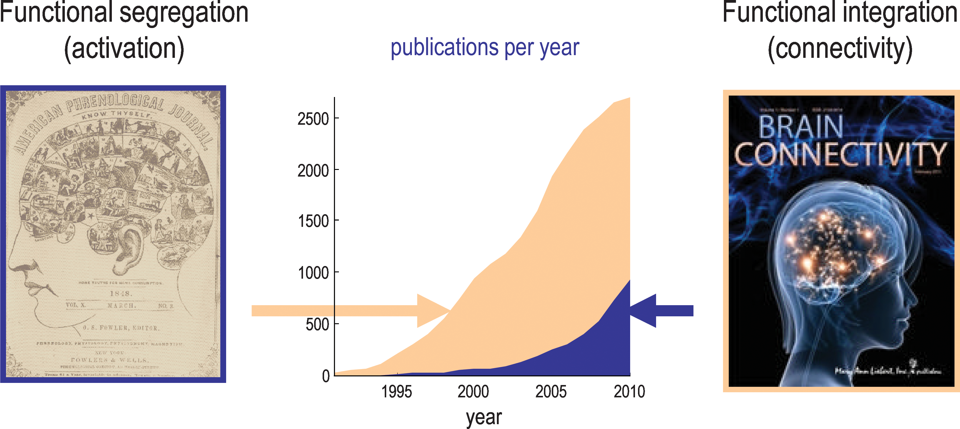
Publication rates pertaining to functional segregation and integration. Publications per year searching for “Activation” or “Connectivity” and functional imaging. This reflects the proportion of studies looking at functional segregation (activation) and those looking at integration (connectivity). Source: PubMed.gov. U.S. National Library of Medicine. The image on the left is from the front cover of The American Phrenological Journal: Vol. 10, No. 3 (March) 1846.
Functional segregation and integration
From a historical perspective, the distinction between functional segregation and functional integration relates to the dialectic between localizationism and connectionism that dominated ideas about brain function in the 19th century. Since the formulation of phrenology by Gall, the identification of a particular brain region with a specific function has become a central theme in neuroscience. Somewhat ironically, the notion that distinct brain functions could be localized was strengthened by early attempts to refute phrenology. In 1808, a scientific committee of the Athénée at Paris, chaired by Cuvier, declared that phrenology was unscientific and invalid (Staum, 1995). This conclusion may have been influenced by Napoleon Bonaparte (after an unflattering examination of his skull by Gall). During the following decades, lesion and electrical stimulation paradigms were developed to test whether functions could indeed be localized in animals. The initial findings of experiments by Flourens on pigeons were incompatible with phrenologist predictions, but later experiments, including stimulation experiments in dogs and monkeys by Fritsch, Hitzig, and Ferrier, supported the idea that there was a relation between distinct brain regions and specific functions. Further, clinicians like Broca and Wernicke showed that patients with focal brain lesions showed specific impairments. However, it was realized early on that it was difficult to attribute a specific function to a cortical area, given the dependence of cerebral activity on the anatomical connections between distant brain regions. For example, a meeting that took place on August 4, 1881, addressed the difficulties of attributing function to a cortical area given the dependence of cerebral activity on underlying connections (Phillips et al., 1984). This meeting was entitled Localization of Function in the Cortex Cerebri. Goltz (1881), although accepting the results of electrical stimulation in dog and monkey cortex, considered the excitation method inconclusive, in that the movements elicited might have originated in related pathways or current could have spread to distant centers. In short, the excitation method could not be used to infer functional localization because localizationism discounted interactions or functional integration among different brain areas. It was proposed that lesion studies could supplement excitation experiments. Ironically, it was observations on patients with brain lesions several years later (see Absher and Benson, 1993) that led to the concept of disconnection syndromes and the refutation of localizationism as a complete or sufficient account of cortical organization. Functional localization implies that a function can be localized in a cortical area, whereas segregation suggests that a cortical area is specialized for some aspects of perceptual or motor processing, and that this specialization is anatomically segregated within the cortex. The cortical infrastructure supporting a single function may then involve many specialized areas whose union is mediated by the functional integration among them. In this view, functional segregation is only meaningful in the context of functional integration and vice versa.
Functional and effective connectivity
Imaging neuroscience has firmly established functional segregation as a principle of brain organization in humans. The integration of segregated areas has proven more difficult to assess. One approach to characterize integration is in terms of functional connectivity, which is usually inferred on the basis of correlations among measurements of neuronal activity. Functional connectivity is defined as statistical dependencies among remote neurophysiological events. However, correlations can arise in a variety of ways. For example, in multiunit electrode recordings, correlations can result from stimulus-locked transients evoked by a common input or reflect stimulus-induced oscillations mediated by synaptic connections (Gerstein and Perkel, 1969). Integration within a distributed system is usually better understood in terms of effective connectivity: effective connectivity refers explicitly to the influence that one neural system exerts over another, either at a synaptic or population level. Aertsen and Preißl (1991) proposed that “effective connectivity should be understood as the experiment and time-dependent, simplest possible circuit diagram that would replicate the observed timing relationships between the recorded neurons.” This speaks to two important points: effective connectivity is dynamic (activity-dependent), and depends on a model of interactions or coupling.
The operational distinction between functional and effective connectivity is important because it determines the nature of the inferences made about functional integration and the sorts of questions that can be addressed. Although this distinction has played an important role in imaging neuroscience, its origins lie in single-unit electrophysiology (Gerstein and Perkel, 1969). It emerged as an attempt to disambiguate the effects of a (shared) stimulus-evoked response from those induced by neuronal connections between two units. In neuroimaging, the confounding effects of stimulus-evoked responses are replaced by the more general problem of common inputs from other brain areas that are manifest as functional connectivity. In contrast, effective connectivity mediates the influence that one neuronal system exerts on another and, therefore, discounts other influences. We will return to this below.
Coupling and connectivity
Put succinctly, functional connectivity is an observable phenomenon that can be quantified with measures of statistical dependencies, such as correlations, coherence, or transfer entropy. Conversely, effective connectivity corresponds to the parameter of a model that tries to explain observed dependencies (functional connectivity). In this sense, effective connectivity corresponds to the intuitive notion of coupling or directed causal influence. It rests explicitly on a model of that influence. This is crucial because it means that the analysis of effective connectivity can be reduced to model comparison—for example, the comparison of a model with and without a particular connection to infer its presence. In this sense, the analysis of effective connectivity recapitulates the scientific process because each model corresponds to an alternative hypothesis about how observed data were caused. In our context, these hypotheses pertain to causal models of distributed brain responses. We will see below that the role of model comparison becomes central when considering different modeling strategies. The philosophy of causal modeling and effective connectivity should be contrasted with the procedures used to characterize functional connectivity. By definition, functional connectivity does not rest on any model of statistical dependencies among observed responses. This is because functional connectivity is essentially an information theoretic measure that is a function of, and only of, probability distributions over observed multivariate responses. This means that there is no inference about the coupling between two brain regions in functional connectivity analyses: the only model comparison is between statistical dependency and the null model (hypothesis) of no dependency. This is usually assessed with correlation coefficients (or coherence in the frequency domain). This may sound odd to those who have been looking for differences in functional connectivity between different experimental conditions or cohorts. However, as we will see later, this may not be the best way of looking for differences in coupling.
Generative or predictive modeling?
It is worth noting that functional and effective connectivity can be used in very different ways: Effective connectivity is generally used to test hypotheses concerning coupling architectures that have been probed experimentally. Different models of effective connectivity are compared in terms of their (statistical) evidence, given empirical data. This is just evidence-based scientific hypothesis testing. We will see later that this does not necessarily imply a purely hypothesis-led approach to effective connectivity; network discovery can be cast in terms of searches over large model spaces to find a model or network (graph) that has the greatest evidence. Because model evidence is a function of both the model and data, analysis of effective connectivity is both model (hypothesis) and data led. The key aspect of effective connectivity analysis is that it ultimately rests on model comparison or optimization. This contrasts with analysis of functional connectivity, which is essentially descriptive in nature. Functional connectivity analyses usually entail finding the predominant pattern of correlations (e.g., with principal or independent component analysis [ICA]) or establishing that a particular correlation between two areas is significant. This is usually where such analyses end. However, there is an important application of functional connectivity that is becoming increasingly evident in the literature. This is the use of functional connectivity as an endophenotype to predict or classify the group from which a particular subject was sampled (e.g., Craddock et al., 2009).
Indeed, when talking to people about their enthusiasm for resting-state (design-free) analyses of functional connectivity, this predictive application is one that excites them. The appeal of resting-state paradigms is obvious in this context: there are no performance confounds when studying patients who may have functional deficits. In this sense, functional connectivity has a distinct role from effective connectivity. Functional connectivity is being used as a (second-order) data feature to classify subjects or predict some experimental factor. It is important to realize, however, that the resulting classification does not test any hypothesis about differences in brain coupling. The reason for this is subtle but simple: in classification problems, one is trying to establish a mapping from imaging data (physiological consequences) to a diagnostic class (categorical cause). This means that the model comparison pertains to a mapping from consequences to causes and not a generative model mapping from causes to consequences (through hidden neurophysiological states). Only analyses of effective connectivity compare (generative) models of coupling among hidden brain states.
In short, one can associate the generative models of effective connectivity with hypotheses about how the brain works, while analyses of functional connectivity address the more pragmatic issue of how to classify or distinguish subjects given some measurement of distributed brain activity. In the latter setting, functional connectivity simply serves as a useful summary of distributed activity, usually reduced to covariances or correlations among different brain regions. In a later section, we will return to this issue and consider how differences in functional connectivity can arise and how they relate to differences in effective connectivity.
It is interesting to reflect on the possibility that these two distinct agendas (generative modeling and classification) are manifest in the connectivity community. Those people interested in functional brain architectures and effective connectivity have been meeting at the Brain Connectivity Workshop series every year (
Connectivity and the connectome
In the many reviews and summaries of the definitions used in brain connectivity research (e.g., Guye et al., 2008; Sporns, 2007), researchers have often supplemented functional and effective connectivity with structural connectivity. In recent years, the fundamental importance of large-scale anatomical infrastructures that support effective connections for coupling has reemerged in the context of the connectome and attendant graph theoretical treatments (Bassett and Bullmore, 2009; Bullmore and Sporns, 2009; Sporns et al., 2005). This may, in part, reflect the availability of probabilistic tractography measures of extrinsic (between area) connections from diffusion tensor imaging (Behrens and Johansen-Berg, 2005). The status of structural connectivity and its relationship to functional effective connectivity is interesting. I see structural connectivity as furnishing constraints or prior beliefs about effective connectivity. In other words, effective connectivity depends on structural connectivity, but structural connectivity per se is neither a sufficient nor a complete description of connectivity.
I have heard it said that if we had complete access to the connectome, we would understand how the brain works. I suspect that most people would not concur with this; it presupposes that brain connectivity possesses some invariant property that can be captured anatomically. However, this is not the case. Synaptic connections in the brain are in a state of constant flux showing exquisite context-sensitivity and time- or activity-dependent effects (e.g., Saneyoshi et al., 2010). These are manifest over a vast range of timescales, from synaptic depression over a few milliseconds (Abbott et al., 1997) to the maintenance of long-term potentiation over weeks. In particular, there are many biophysical mechanisms that underlie fast, nonlinear “gating” of synaptic inputs, such as voltage-dependent ion channels and phosphorylation of glutamatergic receptors by dopamine (Wolf et al., 2003). Even structural connectivity changes over time, at microscopic (e.g., the cycling of postsynaptic receptors between the cytosol and postsynaptic membrane) and macroscopic (e.g., neurodevelopmental) scales. Indeed, most analyses of effective connectivity focus specifically on context- or condition-specific changes in connectivity that are mediated by changes in cognitive set or unfold over time due to synaptic plasticity. These sorts of effects have motivated the development of nonlinear models of effective connectivity that consider explicitly interactions among synaptic inputs (e.g., Friston et al., 1995; Stephan et al., 2008). In short, connectivity is as transient, adaptive, and context-sensitive as brain activity per se. Therefore, it is unlikely that characterizations of connectivity that ignore this will furnish deep insights into distributed processing. So what is the role of structural connectivity?
Structural constraints on the generative models used for effective connectivity analysis are paramount when specifying plausible models. Further (in principle) they enable more precise parameter estimates and more efficient model comparison. Having said this, there is remarkably little evidence that quantitative structural information about connections helps with inferences about effective connectivity. There may be several reasons for this. First, effective connectivity does not have to be mediated by monosynaptic connections. Second, quantitative information about structural connections may not predict their efficacy. For example, the influence or effective connectivity of the (sparse and slender) ascending neuromodulatory projections from areas like the ventral tegmental area may far exceed the influence predicted by their anatomical prevalence. The only formal work so far that demonstrates the utility of tractography estimates is reported in Stephan et al. (2009). This work compared dynamic causal models of effective connectivity (in a visual interhemispheric integration task) that were and were not informed by structural priors based on tractography. The authors found that models with tractography priors had more evidence than those without them (see Fig. 2 for details). This provides definitive evidence that structural constraints on effective connectivity furnish better models. Crucially, the tractography priors were not on the strength of the connections, but on the precision or uncertainty about their strength. In other words, structural connectivity was shown to play a permissive role as a prior belief about effective connectivity. This is important because it means that the existence of a structural connection means (operationally) that the underlying coupling may or may not be expressed.

Structural constraints on functional connections. This schematic illustrates the procedure reported in Stephan et al. (2009), providing evidence that anatomical tractography measures provide informative constraints on models and effective connectivity. Consider the problem of estimating the effective connectivity among some regions, given quantitative (if probabilistic) estimates of their anatomical connection strengths (demoted by φij ). This is illustrated in the lower left panel using bilateral areas in the lingual and fusiform gyri. The first step would be to specify some mapping between the anatomical information and prior beliefs about the effective connections. This mapping is illustrated in the upper left panel, by expressing the prior variance on effective connectivity (model parameters θ) as a sigmoid function of anatomical connectivity, with unknown hyperparameters α β ⊂ m, where m denotes a model. We can now optimize the model in terms of its hyperparameters and select the model with the highest evidence p(y|m), as illustrated by model scoring on the upper right. When this was done using empirical data, tractography priors were found to have a sensible and quantitatively important role. The inset on the lower right shows the optimum relationship between tractography estimates and prior variance constraints on effective connectivity. The four asterisks correspond to the four tractography measures shown on the lower left [see Stephan et al. (2009) for further detail].
A potentially exciting development in diffusion tensor imaging is the ability to invert generative models of axonal structure to recover much more detailed information about the nature of the underlying connections (Alexander, 2008). A nice example here is that if we were able to estimate the diameter of extrinsic axonal connections between two areas (Zhang and Alexander, 2010), this might provide useful priors on their conduction velocity (or delays). Conduction delays are a free parameter of generative models for electrophysiological responses (see below). This raises the possibility of establishing structure–function relationships in connectivity research, at the microscopic level, using noninvasive techniques. This is an exciting prospect that several of my colleagues are currently pursuing.
Summary
This section has introduced the distinction between functional segregation and integration in the brain and how the differences between functional and effective connectivity shape the way we characterize connections and the sorts of questions that are addressed. We have touched upon the role of structural connectivity in providing constraints on the expression of effective connectivity or coupling among neuronal systems. In the next section, we look at the relationship between functional and effective connectivity and how the former depends upon the latter.
Analyzing Connectivity
This section looks more formally at functional and effective connectivity, starting with a generic (state-space) model of the neuronal systems that we are trying to characterize. This necessarily entails a generative model and, implicitly, frames the problem in terms of effective connectivity. We will look at ways of identifying the parameters of these models and comparing different models statistically. In particular, we will consider successive approximations that lead to simpler models and procedures commonly employed to analyze connectivity. In doing this, we will hopefully see the relationships among the different analyses and the assumptions on which they rest. To make this section as clear as possible, it will use a toy example to quantify the implications of various assumptions. This example uses a plausible connectivity architecture and shows how changes in coupling, under different experimental conditions or cohorts, would be manifest as changes in effective or functional connectivity. This section concludes with a heuristic discussion of how to compare connectivity between conditions or groups. The material here is a bit technical but uses a tutorial style that tries to suppress unnecessary mathematical details (with a slight loss of rigor and generality).
A generative model of coupled neuronal systems
We start with a generic description of distributed neuronal and other physiological dynamics, in terms of differential equations. These equations describe the motion or flow, f(x, u, θ), of hidden neuronal and physiological states, x(t), such as synaptic activity and blood volume. These states are hidden because they are not observed directly. This means we also have to specify mapping, g(x, u, θ), from hidden states to observed responses, y(t):
Here, u(t) corresponds to exogenous inputs that might encode changes in experimental conditions or the context under which the responses were observed. Random fluctuations ω(t) and v(t) on the motion of hidden states and observations render Equation (1) a random or stochastic differential equation. One might wonder why we need both exogenous (deterministic) and endogenous (random) inputs; whereas the exogenous inputs are generally known and under experimental control, endogenous inputs represent unknown influences (e.g., from areas not in the model or spontaneous fluctuations). These can only be modeled probabilistically (usually under Gaussian, and possibly Markovian, assumptions).
Clearly, the equations of motion (first equality) and observer function (second equality) are, in reality, immensely complicated equations of very large numbers of hidden states. In practice, there are various theorems such as the center manifold theorem* and slaving principle, which means one can reduce the effective number of hidden states substantially but still retain the underlying dynamical structure of the system (Ginzburg and Landau, 1950; Carr, 1981; Haken, 1983; Kopell and Ermentrout, 1986). The parameters of these equations, θ, include effective connectivity and control how hidden states in one part of the brain affect the motion of hidden states elsewhere. Equation (1) can be regarded as a generative model of observed data that is specified completely, given assumptions about the random fluctuations and prior beliefs about the states and parameters. Inverting or fitting this generative model corresponds to estimating its unknown states and parameters (effective connectivity), given some observed data. This is called dynamic causal modeling (DCM) and usually employs Bayesian techniques.
However, the real power of DCM lies in the ability to compare different models of the same data. This comparison rests on the model evidence, which is simply the probability of the observed data, under the model in question (and known exogenous inputs). The evidence is also called the marginal likelihood because one marginalizes or removes dependencies on the unknown quantities (states and parameters).
Model comparison rests on the relative evidence for one model compared to another [see Penny et al. (2004) for a discussion in the context of functional magnetic resonance imaging (fMRI). Likelihood-ratio tests of this sort are commonplace. Indeed, one can cast the t-statistic as a likelihood ratio. Model comparison based on the likelihood of different models will be a central theme in this review and provides the quantitative basis for all evidence-based hypothesis testing. In this section, we will see that all analyses of effective connectivity can be reduced to model comparison. This means the crucial differences among these analyses rest with the models on which they are based.
Clearly, to search over all possible models (to find the one with the most evidence) is generally impossible. One, therefore, appeals to simplified but plausible models. To illustrate this simplification and to create an illustrative toy example, we will use a local (bilinear) approximation to Equation (1) of the sort used in DCM of fMRI time series (Friston et al., 2003) and with a single exogenous input,
Here, superscripts indicate whether the parameters refer to the strength of connections, θx
, their context-dependent (bilinear) modulation, θxu
, or the effects of perturbations or exogenous inputs, θu
. To keep things very simple, we will further pretend that we have direct access to hidden neuronal states and that they are measured directly (as in invasive electrophysiology). This means we can ignore hemodynamics and the observer function (for now). Equation (3) parameterizes connectivity in terms of partial derivatives of the state-equation. For example, the network in Figure 3 can be described with the following effective connectivity parameters:

Toy connectivity architecture. This schematic shows the connections among three brain areas or nodes that will be used to demonstrate the relationship between effective connectivity and functional connectivity in the main text. To highlight the role of changes in connectivity, the right graph shows the connection that changes (over experimental condition or diagnostic cohort) as the thick black line. This is an example of a directed cyclic graph. It is cyclic by virtue of the reciprocal connections between A1 and A2.
Here, the input
Dynamic causal modeling
As noted above, DCM would first select the best model using Bayesian model comparison. Usually, different models are specified in terms of priors on the coupling parameters. These are used to switch off parameters by assuming a priori that they are zero (to create a new model). For example, if we wanted to test for the presence of a backward connection from the second to the first area,
These Gaussian (shrinkage) priors force the effective connectivity to be zero under the null model m
0 and allow it to take large values under m
1. Given sufficient data, the Bayesian model comparison would confirm that the evidence for the alternative model was greater than the null model, using the logarithm of the evidence ratio:
Notice that we have expressed the logarithm of the marginal likelihood ratio as a difference in log-evidences. This is a preferred form because model comparison is not limited to two models, but can cover a large number of models whose quality can be usefully quantified in terms of their log-evidences. (We will see an example of this in the last section.) A relative log-evidence of three corresponds to a marginal likelihood ratio (Bayes factor) of about 20 to 1, which is usually considered strong evidence in favor of one model over another (Kass and Raftery, 1995). An important aspect of model evidence is that it includes a complexity cost (which is not only sensitive to the number of parameters but also to their interdependence). This means that a model with redundant parameters would have less evidence, even though it provided a better fit to the data (see Penny et al., 2004).
In most current implementations of DCM, the log-evidence is approximated with a (variational) free-energy bound that (by construction) is always less than the log-evidence. This bound is a function of the data and (under Gaussian assumptions about the posterior density) some proposed values for the states and parameters. When the free-energy is maximized (using gradient ascent) with respect to the proposed values, they become the maximum posterior or conditional estimates, μ, and the free-energy,
Vector autoregression models and Granger causality
One can convert any dynamic causal model into a linear state-space or vector autoregression model (Goebel et al., 2003; Harrison et al., 2003; see Rogers et al., 2010 for review) by solving (integrating) the Taylor approximation to Equation (3) over the intervals between data samples, Δ, using the matrix exponential. For a single experimental context (the first input level, u=0), this gives:
The second equality expresses this vector autoregression model as a simple general linear model with explanatory variables,
We now have a new model whose parameters are autoregression coefficients that can be tested using classical likelihood ratio tests. In other words, we can compare the likelihood of models with and without a particular regression coefficient, Aij
, using classical model comparison based on the extra sum of squares principle (e.g., the F-statistic). For n states and ɛ∼N (0, σ
2 I), these tests are based on the sum of squares and products of the residuals, Ri
: i=0,1, under the maximum likelihood solutions of the alternative and null models, respectively:
This is Granger causality (Granger, 1969) and has been used in the context of autoregressive models of fMRI data (Roebroeck et al., 2005, 2009). Note that Equation (8) uses likelihoods as opposed to marginal likelihoods to approximate the evidence. This (ubiquitous) form of model comparison assumes that the posterior density over unknown quantities can be approximated by a point mass over the conditional mean. In the absence of priors, this is their maximum likelihood value. In other words, we ignore uncertainty about the parameters when estimating the evidence for different models. This is a reasonable heuristic but fails to account for differences in model complexity (which means the approximation in Equation (8) is never less than zero).
The likelihood model used in tests of Granger causality assumes that the random terms in the vector autoregression model are (serially) independent. This is slightly problematic given that these terms acquire temporal correlations when converting the continuous time formulation into the discrete time formulation [see Equation (7)]. The independence (Markovian) assumption means that the network has forgotten past fluctuations by the time it is next sampled (i.e., it is not sampled very quickly). However, there is a more fundamental problem with Granger causality that rests on the fact that the autoregression parameters of Equation (7) are not the coupling parameters of Equation (3). In our toy example, with a repetition time of Δ=2.4 seconds, the true autoregression coefficients are
This means, with sufficient data, area
There are many other interesting debates about the use of Granger causality in fMRI time series analysis [see Valdés-Sosa et al. (2011) for a full discussion of these issues]. Many relate to the effects of hemodynamic convolution, which is ignored in most applications of Granger causality (see Chang et al., 2008; David et al., 2008). A list of the assumptions entailed by the use of a linear autoregression model for fMRI includes • The hemodynamic response function is identical in all regions studied. • The hemodynamic response is measured with no noise. • Neuronal dynamics are linear with no changes in coupling. • Neuronal innovations (fluctuations) are stationary. • Neuronal innovations (fluctuations) are Markovian. • The sampling interval (TR) is smaller than the time constants of neuronal dynamics. • The sampling interval (TR) is greater than the time constants of the innovations.
It is clear that these assumptions are violated in fMRI and that Granger causality calls for some scrutiny. Indeed, a recent study (Smith et al., 2010) used simulated fMRI time series to compare Granger causality against a series of procedures based on functional connectivity (partial correlations, mutual information, coherence, generalized synchrony, and Bayesian networks; e.g., Baccalá and Sameshima, 2001; Marrelec et al., 2006; Patel et al., 2006). They found that Granger causality (and its frequency domain variants, such as directed partial coherence and directed transfer functions; e.g., Geweke, 1984) performed poorly and noted that The spurious causality estimation that is still seen in the absence of hemodynamic response function variability most likely relates to the various problems described in the Granger literature (Nalatore et al., 2007; Nolte et al., 2008; Tiao and Wei, 1976; Wei, 1978; Weiss, 1984); it is known that measurement noise can reverse the estimation of causality direction, and the temporal smoothing means that correlated time series are estimated to [Granger] “cause” each other.
It should be noted that the deeper mathematical theory of Granger causality (due to Wiener, Akaike, Granger, and Schweder) transcends its application to a particular model (e.g., the linear autoregression model above). Having said this, each clever refinement and generalization of Granger causality (e.g., Deshpande et al., 2010; Havlicek et al., 2010; Marinazzo et al., 2010) brings it one step closer to DCM (at least from my point of view). As noted above, autoregression models assume the innovations are temporally uncorrelated. In other words, random fluctuations are fast, in relation to neuronal dynamics. We will now make the opposite assumption, which leads to the models that underlie structural equation modeling.
Structural equation modeling
If we now use an adiabatic approximation† and assume that neuronal dynamics are very fast in relation to random fluctuations, we can simplify the model above by removing the dynamics. In other words, we can assume that neuronal activity has reached steady-state by the time we observe it. The key advantage of this is that we can reduce the generative model so that it predicts, not the time series, but the observed covariances among regional responses over time, Σy .
For simplicity, we will assume that g(x, y, θ)=x and u=0. If the rate of change of hidden states is zero, Eqs. (1) and (3) mean that
Expressing the covariances in terms of the coupling parameters enables one to compare structural equation models using likelihoods based on the observed sample covariances.
The requisite maximum likelihood estimates of the coupling and covariance parameters, μ, can now be estimated in a relatively straightforward manner, using standard covariance component estimation techniques. Note that we do not have to estimate hidden states because the generative model explains observed covariances in terms of random fluctuations and unknown coupling parameters [see Equation (10)]. The form of Equation (10) has been derived from the generic generative model. In this form, it can be regarded as a Gaussian process model, where the coupling parameters become, effectively, parameters of the covariance among observed signals due to hidden states. Although we have derived this model from differential equations, structural equation modeling is usually described as a regression analysis. We can recover the implicit regression model in Equation (10) by separating the intrinsic or self-connections (which we will assume to be modeled by the identity matrix) and the off-diagonal terms. This gives an instantaneous regression model, θx =θ − I ⇒ x=θx + ω, whose maximum likelihood parameters can be estimated in the usual way (under appropriate constraints).
So, is this a useful way to characterize effective connectivity in an imaging time series? The answer to this question depends on the adiabatic assumption that converts the dynamic model into a static model. Effectively, one assumes that random fluctuations change very slowly in relation to underlying physiology, such that it has time to reach steady state. Clearly, this is not appropriate for electrophysiological and fMRI time series, where the characteristic time constants of neuronal dynamics (tens of milliseconds) and hemodynamics (seconds) are generally much larger than the fluctuating or exogenous inputs that drive them. This is especially true when eliciting neuronal responses using event-related designs. Having said this, structural equation modeling may have a useful role in characterizing nontime-series data, such as the gray matter segments analyzed in voxel-based morphometry or images of cerebral metabolism acquired with positron emission tomography. Indeed, it was in this setting that structural equation modeling was introduced to neuroimaging: The first application of structural equation modeling used 2-deoxyglucose images of the rat auditory system (McIntosh and Gonzalez-Lima, 1991), followed by a series of applications to positron emission tomography data (McIntosh et al., 1994; see also Protzner and McIntosh, 2006).
There is a further problem with using structural equation modeling in the analysis of effective connectivity: it is difficult to estimate reciprocal and cyclic connections efficiently. Intuitively, this is because fitting the sample covariance means that we have thrown away a lot of information in the original time series. Heuristically, the ensuing loss of degrees of freedom means that conditional dependencies among the estimates of effective connectivity are less easy to resolve. This means that, typically, one restricts analyse to simple networks that are nearly acyclic (or, in the special case of path analysis, fully acyclic), with a limited number of loops that can be identified with a high degree of statistical precision. In machine learning, structural equation modeling can be regarded as a generalization of inference on linear Gaussian Bayesian networks that relaxes the acyclic constraint. As such, it is a generalization of structural causal modeling, which deals with directed acyclic graphics. This generalization is important in the neurosciences because of the ubiquitous reciprocal connections in the brain that render its connectivity cyclic or recursive. We will return to this point when we consider structural causal modeling in the next section.
Functional connectivity and correlations
So far, we have considered procedures for identifying effective connectivity. So, what is the relationship between functional connectivity and effective connectivity? Almost universally in fMRI, functional connectivity is assessed with the correlation coefficient. These correlations are related mathematically to effective connectivity in the following way (for simplicity, we will again assume that g(x, y, θ)=x and u=0):
These equations show that correlation is based on the covariances over regions, where these covariances are induced by observation noise and random fluctuations. Crucially, because the system has memory, we have to consider the history of the fluctuations causing observed correlations. The effect of past fluctuations is mediated by the kernels, exp(τθx
), in Equation (12). The Fourier transforms of these kernels (transfer functions) can be used to compute the coherence among regions at any particular frequency. In our toy example, the functional connections for the two experimental contexts are (for equal covariance among random fluctuations and observation noise, Σω
=Σv
=1):
There are two key observations here. First, although there is no coupling between the second and third area, they show a profound functional connectivity as evidenced by the correlations between them in both contexts (0.41 and 0.769, respectively). This is an important point that illustrates the problem of common input (from the first area) that the original distinction between functional and effective connectivity tried to address (Gerstein and Perkel, 1969). Second, despite the fact that the only difference between the two networks lies in one (backward) connection (from the second to the first area), this single change has produced large and distributed changes in functional connectivity throughout the network. We will return to this issue below when commenting on the comparison of connection strengths. First, we consider briefly the different ways in which distributed correlations can be characterized.
Correlations, components, and modes
From the perspective of generative modeling, correlations are data features that summarize statistical dependencies among brain regions. As such, one would not consider model comparison because the correlations are attributes of the data, not the model. In this sense, functional connectivity can be regarded as descriptive. In general, the simplest way to summarize a pattern of correlations is to report their eigenvectors or principal components. Indeed, this is how voxel-wise functional connectivity was introduced (Friston et al., 1993). Eigenvectors correspond to spatial patterns or modes that capture, in a step down fashion, the largest amount of observed covariance. Principal component analysis is also known as the Karhunen-Loève transform, proper orthogonal decomposition, or the Hotelling transform. The principal components of our simple example (for the first context) are the following columns:
When applying the same analysis to resting-state correlations, these columns would correspond to the weights that define intrinsic brain networks (Van Dijk et al., 2010). In general, the weights of a mode can be positive and negative, indicating those regions that go up and down together over time. In Karhunen-Loève transforms of electrophysiological time series, this presents no problem because positive and negative changes in voltage are treated on an equal footing. However, in fMRI research, there appears to have emerged a rather quirky separation of the positive and negative parts of a spatial mode (e.g., Fox et al., 2009) that are anticorrelated (i.e., have a negative correlation). This may reflect the fact that the physiological interpretation of activation and deactivation is not completely symmetrical in fMRI. Another explanation may be related to the fact that spatial modes are often identified using spatial independent component analysis (ICA).
Independent component analysis
ICA has very similar objectives to principal component analysis (PCA), but assumes the modes are driven by non-Gaussian random fluctuations (Calhoun and Adali, 2006; Kiviniemi et al., 2003; McKeown et al., 1998). If we reprieve the assumptions of structural equation modeling [Equation (10)], we can regard principal component analysis as based up the following generative model:
By simply replacing Gaussian assumptions about random fluctuations with non-Gaussian (supra-Gaussian) assumptions, we can obtain the generative model on which ICA is based. The aim of ICA is to identify the maximum likelihood estimates of the mixing matrix, W=(θx )−1, given observed covariances. These correspond to the modes above. However, when performing ICA over voxels in fMRI, there is one final twist. For computational reasons, it is easier to analyze sample correlations over voxels than to analyze the enormous (voxel×voxel) matrix of correlations over time. Analyzing the smaller (time×time) matrix is known as spatial ICA (McKeown et al., 1998). [See Friston (1998) for an early discussion of the relative merits of spatial and temporal ICA.] In the present context, this means that the modes are independent (and orthogonal) over space and that the temporal expression of these independent components may be correlated. Put plainly, this means that independent components obtained by spatial ICA may or may not be functionally connected in time. I make this point because those from outside the fMRI community may be confused by the assertion that two spatial modes (intrinsic brain networks) are anticorrelated. This is because they might assume temporal ICA (or PCA) was used to identify the modes, which are (by definition) uncorrelated.
Changes in connectivity
So far, we have focused on comparing different models or network architectures that best explain observed data. We now look more closely at inferring quantitative changes in coupling due to experimental manipulations. As noted above, there is a profound difference between comparing effective connection strengths and functional connectivity. In effective connectivity modeling, one usually makes inferences about coupling changes by comparing models with and without an effect of experimental context or cohort. These effects correspond to the bilinear parameters θxu in Equation (3). If model comparison supported the evidence for the model with a context or cohort effect, one would then conclude the associated connection (or connections) had changed. However, when comparing functional connectivity, one cannot make any comment about changes in coupling. Basically, showing that there is a difference in the correlation between two areas does not mean that the coupling between these areas has changed; it only means that there has been some change in the distributed activity observed in one context and another and that this change is manifest in the correlation [see Equation (13)]. Clearly, this is not a problem if one is only interested in using correlations to predict the cohort or condition from which data were sampled. However, it is important not to interpret a difference in correlation as a change in coupling. The correlation coefficient reports the evidence for a statistical dependency between two areas, but changes in this dependency can arise without changes in coupling. This is particularly important for Granger causality, where it might be tempting to compare Granger causality, either between two experimental situations or between directed connections between two nodes. In short, a difference in evidence (correlation, coherence, or Granger causality) should not be taken as evidence for a difference in coupling. One can illustrate this important point with three examples of how a change in correlation could be observed in the absence of a change in effective connectivity.
Changes in another connection
Because functional connectivity can be expressed at a distance from changes in effective connectivity, any observed change in the correlation between two areas can be easily caused by a coupling change elsewhere. Using our example above, we can see immediately that the correlation between
This is perfectly sensible and reflects the fact that statistical dependencies among the nodes of a network are exquisitely sensitive to changes in coupling anywhere. So, does this mean a change in a correlation can be used to infer a change in coupling somewhere in the system? No, because the correlation can change without any change in coupling.
Changes in the level of observation noise
An important fallacy of comparing correlation coefficients rests on the fact that correlations depend on the level of observation noise. This means that one can see a change in correlation by simply changing the signal-to-noise ratio of the data. This can be particularly important when comparing correlations between different groups of subjects. For example, obsessive compulsive patients may have a heart rate variability that differs from normal subjects. This may change the noise in observed hemodynamic responses, even in the absence of neuronal differences or changes in effective connectivity. We can simulate this effect, using Equation (12) above, where, using noise levels of Σv
=1 and Σv
=1.252, we obtain the following difference in correlations:
These changes are just due to increasing the standard deviation of observation noise by 25%. This reduces the correlation because it changes with the noise level [see Equation (12)]. The ensuing difficulties associated with comparing correlations are well known in statistics and are related to the problem of dilution or attenuation in regression problems (e.g., Spearman, 1904). If we ensured that the observation noise was the same over different levels of an experimental factor, could we then infer some change in the underlying connectivity? Again, the answer is no because the correlation also depends on the variance of hidden neuronal states, Σω , that can only be estimated under a generative model.
Changes in neuronal fluctuations
One can produce the same sort of difference in correlations by changing the amplitude of neuronal fluctuations (designed or endogenous) without changing the coupling. As a quantitative example, from Equation (12) we obtain the following difference in correlations when changing Σω
=1 to Σω
=1.252:
The possible explanations for differences in neuronal activity between different cohorts of subjects, or indeed different conditions, are obviously innumerable. Yet, any of these differences can produce a change in functional connectivity.
These examples highlight the difficulties of interpreting differences in functional connectivity in relation to changes in the underlying coupling. Importantly, these arguments pertain to any measures reporting the evidence for statistical dependencies, including coherence, mutual information, transfer entropy, and Granger causality. The fallacy of comparing statistics in this way can be seen intuitively in terms of model comparison. Usually, one compares the evidence for different models of the same data. When testing for a change in coupling, this entails comparing models that do and do not include a change in connectivity. This is not the same as comparing the evidence for the same model of different data. A change in evidence here simply means the data have changed. In short, a change in model evidence is not evidence for model of change.
As noted above, these interpretational issues may not be relevant when simply trying to establish group differences or classify subjects. However, if one wants to make some specific and mechanistic inference about the impact of an experimental manipulation on the coupling between particular brain regions, he or she has to use effective connectivity. Happily, there is a relatively straightforward way of doing this for fMRI that is less complicated than comparing correlations.
Psychophysiological interactions
Assume that we wanted to test the hypothesis that fronto-temporal coupling differed significantly between two groups of subjects. Given the above arguments, we would compare models of effective connectivity that did and did not allow for a change. One of the most basic model comparisons that can be implemented using standard linear convolution models for fMRI is the test for a psychophysiological interaction. In this comparison, one tests for interactions between a physiological variable and a psychological variable or experimental factor. This interaction is generally interpreted in terms of an experimentally mediated change in (linear) effective connectivity between the area expressing a significant interaction and the seed or reference region from which the physiological variable was harvested. At the between-subject or group level, this reduces to a group difference between the regression coefficient that is obtained from regressing the activity at any point in the brain on the activity of the seed region [see Kasahara et al. (2010) for a nice application]. It is this regression coefficient that can be associated with effective connectivity (i.e., change in activity per unit change in the seed region). To test the null hypothesis that there is no group difference in coupling, one simply performs a two sample t-test on the regression coefficients. The results of this whole-brain analysis can be treated in the usual way to identify those regions whose effective connectivity with the reference region differs significantly.
Note that this is very similar to a comparison of correlations with a seed region. The crucial difference is that the summary statistic (summarizing the connectivity) reports effective connectivity, not functional connectivity. This means that it is not confounded by differences in signal or noise, and (under the simple assumptions of a psychophysiological interaction model) can be interpreted as a change in coupling. It should be said that there are many qualifications to the use of these simple linear models of effective connectivity (because they belong to the class of structural equation or regression models; Friston et al., 1997). However, psychophysiologic interactions are simple, intuitive, and (mildly) principled. Further, because the fluctuations in the physiological measure are typically slow in resting-state studies, the usual caveats of hemodynamic convolution can be ignored.
Summary
This section has tried to place different analyses of connectivity in relation to each other. The most prevalent approaches to effective connectivity analysis are DCM, structural equation modeling, and Granger causality. All have enjoyed a rapid uptake over the past decade (see Fig. 4). This didactic (and polemic) treatment has highlighted some of the implicit and implausible assumptions made when applying structural equation modeling and Granger causality to fMRI time series. I personally find the recent upsurge of Granger causality in fMRI worrisome, and it is difficult to know what to do when asked to review these articles. In practice, I generally just ask authors to qualify their conclusions by listing the assumptions that underlie their analysis. On the one hand, it is important that people are not discouraged from advancing and applying classical time series analyses to fMRI. On the other hand, the persistent use of models and procedures that are not fit for purpose may confound scientific progress in the long term. Perhaps, having written this, people will exclude me from reviewing their articles on Granger causality and I will no longer have to worry about these things. On a more constructive note, casting Granger causality as a time-finessed measure of functional connectivity may highlight its potentially useful role in identifying distributed networks for subsequent analyses of effective connectivity.
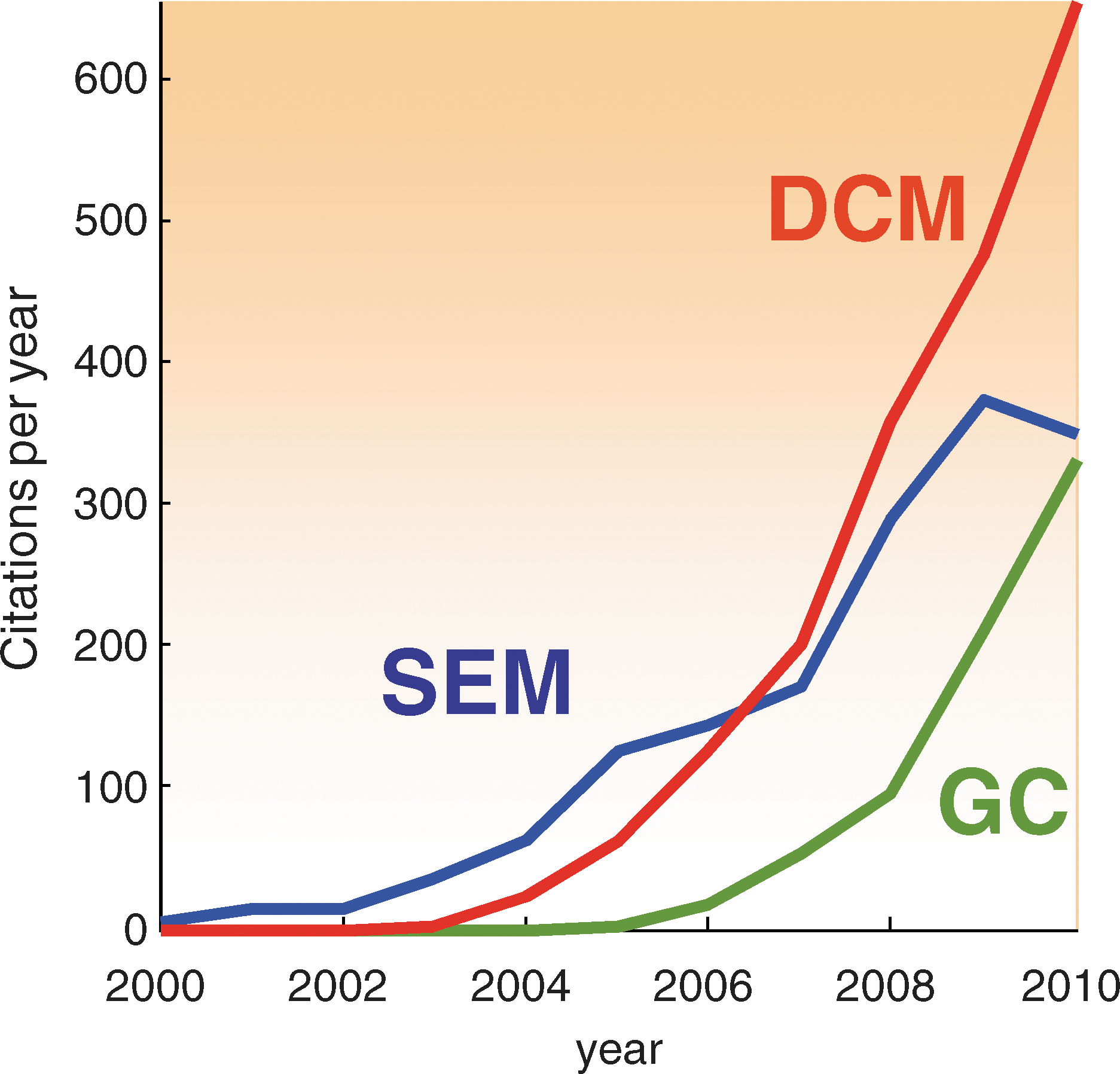
Citation rates pertaining to effective connectivity analyses. Citations per year searching for Dynamic causal mode[l]ling and fMRI, structural equation mode[l]ling and fMRI and Granger causality and fMRI (under Topic=Neurosciences). These profiles reflect the accelerating use of modern time-series analyses to characterize effective connectivity. DCM, dynamic causal modeling; SEM, structural equation modeling; GC, Granger causality; fMRI, functional magnetic resonance imaging. Source: ISI Web of Knowledge.
In summary, we have considered some of the practical issues that attend the analysis of functional and effective connectivity and have exposed the assumptions on which different approaches are based. We have seen that there is a complicated relationship between functional connectivity and the underlying effective connectivity. We have touched on the difficulties of interpreting differences in correlations and have described one simple solution. In the remainder of this review, we will focus on generative models of distributed brain responses and consider some of the exciting developments in this field.
Modeling Distributed Neuronal Systems
This section considers the modeling of distributed dynamics in more general terms. Biophysical models of neuronal dynamics are usually used for one of two things: either to understand the emergent properties of neuronal systems or as observation models for measured neuronal responses. We discuss examples of both. In terms of emergent behaviors, we will consider dynamics on structure (Bressler and Tognoli, 2006; Buice and Cowan, 2009; Coombes and Doole, 1996; Freeman, 1994, 2005; Kriener et al., 2008; Robinson et al., 1997; Rubinov et al., 2009; Tsuda, 2001) and how this behavior has been applied to characterizing autonomous or endogenous fluctuations in fMRI (e.g., Deco et al., 2009, 2011; Ghosh et al., 2008; Honey et al., 2007, 2009). We will then consider causal models that are used to explain empirical observations. This section concludes with recent advances in DCM of directed neuronal interactions that support endogenous fluctuations. The first half of this section is based on Friston and Dolan (2010), to which readers are referred for more detail.
Modeling autonomous dynamics
There has been a recent upsurge in studies of fMRI signal correlations observed while the brain is at rest (Biswal et al., 1995). These patterns reflect anatomical connectivity (Greicius et al., 2009; Pawela et al., 2008) and can be characterized in terms of remarkably reproducible spatial modes (resting-state or intrinsic networks). One of these modes recapitulates the pattern of deactivations observed across a range of activation studies (the default mode; Raichle et al., 2001). These studies show that even at rest endogenous brain activity is self-organizing and highly structured. There are many questions about the genesis of autonomous dynamics and the structures that support them. Some of the more interesting come from computational anatomy and neuroscience. The emerging picture is that endogenous fluctuations are a consequence of dynamics on anatomical connectivity structures with particular scale-invariant and small-world characteristics (Achard et al., 2006; Bassett et al., 2006; Deco et al., 2009; Honey et al., 2007). These are well-studied and universal characteristics of complex systems and suggest that we may be able to understand the brain in terms of universal phenomena (Sporns, 2010). For example, Buice and Cowan (2009) model neocortical dynamics using field-theoretic methods (from nonequilibrium statistical processes) to describe both neural fluctuations and responses to stimuli. In their models, the density and extent of lateral cortical interactions induce a region of state space, in which the effects of fluctuations are negligible. However, as the generation and decay of neuronal activity comes into balance, there is a transition into a regime of critical fluctuations. These models suggest that the scaling laws found in many measurements of neocortical activity are consistent with the existence of phase-transitions at a critical point. They also speak to larger questions about how the brain maintains itself near phase-transitions (i.e., self-organized criticality and gain control; Abbott et al., 1997; Kitzbichler et al., 2009). This is an important issue because systems near phase-transitions show universal phenomena (Jirsa et al., 1994; Jirsa and Haken, 1996; Jirsa and Kelso, 2000; Tognoli and Kelso, 2009; Tschacher and Haken, 2007). Although many people argue for criticality and power law effects in large-scale cortical activity (e.g., Freyer et al., 2009; Kitzbichler et al., 2009; Linkenkaer-Hansen et al., 2001; Stam and de Bruin, 2004), other people do not (Bedard et al., 2006; Miller et al., 2007; Touboul and Destexhe, 2009). It may be that slow (electrophysiological) frequencies contain critical oscillations, whereas high-frequency coherent oscillations may reflect other dynamical processes. In summary, endogenous fluctuations may be one way in which anatomy is expressed through dynamics. They also pose interesting questions about how fluctuations shape evoked responses (e.g., Hesselmann et al., 2008) and vice versa (e.g., Bianciardi et al., 2009).
Dynamical approaches to understanding phenomena in neuroimaging data focus on emergent behaviors and the constraints under which brain-like behaviors manifest (e.g., Breakspear and Stam, 2005; Alstott et al., 2009). In the remainder of this section, we turn to models that try to explain observed neuronal activity directly. This rests on model fitting or inversion. Model inversion is important. To date, most efforts in computational neuroscience have focused on generative models of neuronal dynamics (which define a mapping from causes to neuronal dynamics). The inversion of these models (the mapping from neuronal dynamics to their causes) now allows one to test different models against empirical data. This is best exemplified by model selection as discussed in the previous section. In what follows, we will consider two key classes of probabilistic generative models—namely, structural and dynamic causal models.
Structural causal modeling
As noted by Valdés-Sosa et al. (2011), “despite philosophical disagreements about the study of causality, there seems to be a consensus that causal modeling is a legitimate statistical enterprise.” One can differentiate two streams of statistical causal modeling: one based on Bayesian dependency graphs or graphical models called structural causal modeling (White and Lu, 2010), and the other based on causal influences over time, which we will consider under DCM (see Fig. 5).
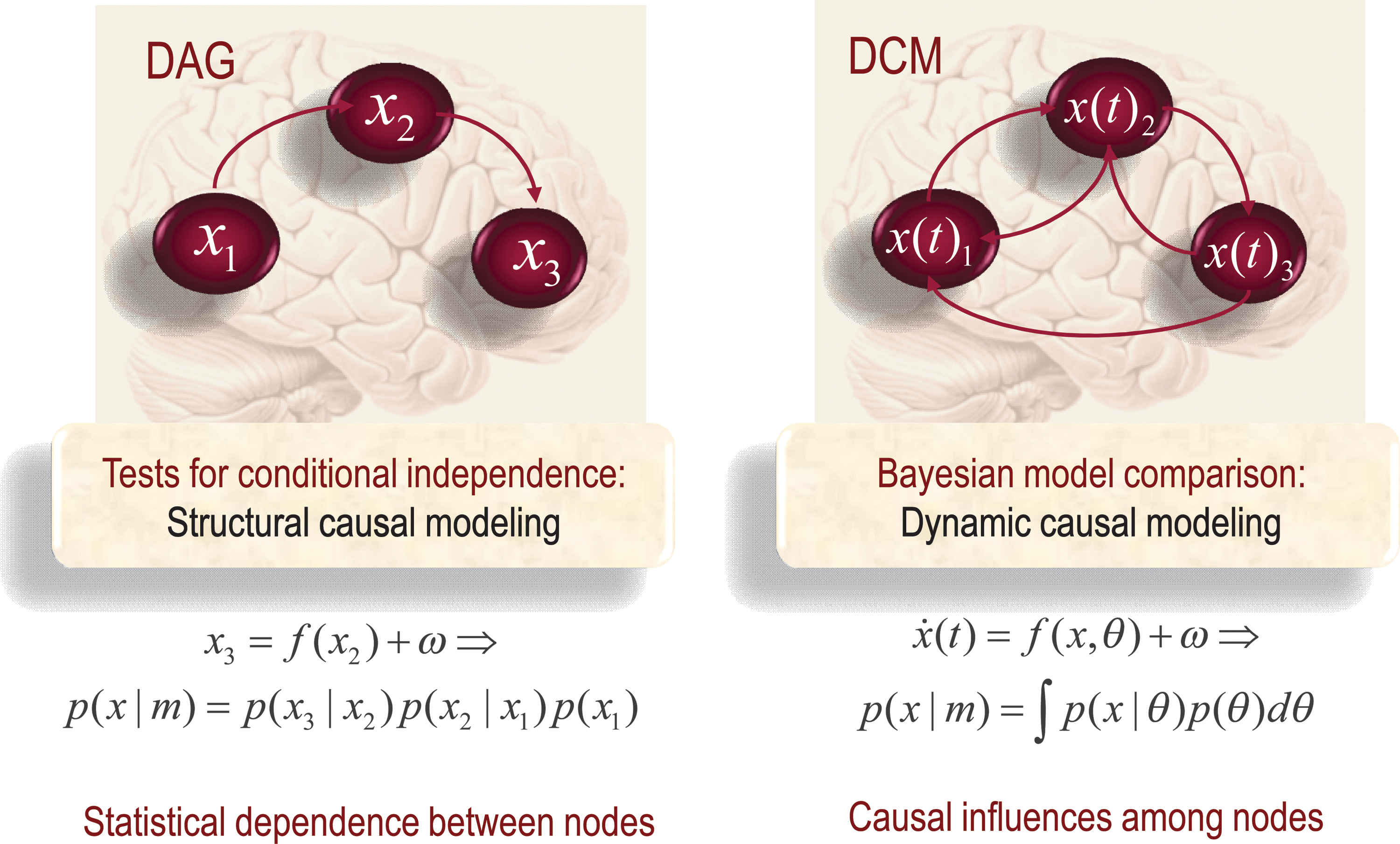
Structural and dynamic causal modeling. Schematic highlighting the distinctions between structural and dynamic causal modeling; these are closely related to the distinction between functional effective connectivity, in the sense that structural equation modeling is concerned principally with conditional dependencies induced by static nonlinear mappings. Conversely, DCM is based explicitly on differential equations that embody causality in a control theory or intuitive sense. DAG, directed a cyclic graph; DCM, dynamic causal model or directed cyclic model.
Graphical models and Bayesian networks
Structural causal modeling originated with structural equation modeling (Wright, 1921) and uses graphical models (Bayesian dependency graphs or Bayes nets) in which direct causal links are encoded by directed edges (Lauritzen, 1996; Pearl, 2000; Spirtes et al., 2000). Model comparison procedures are then used to discover the best model (graph) given some data. However, there may be many models with the same evidence. In this case, the search produces an equivalence class of models with the same explanatory power. This degeneracy has been highlighted by Ramsey et al. (2010) in the setting of effective connectivity analysis.
An essential part of network discovery in structural causal modeling is the concept of intervention—namely, eliminating connections in the graph and setting certain nodes to given values. The causal calculus based on graphical models has some important connections to the distinction between functional and effective connectivity and provides an elegant framework within which one can deal with interventions. However, it is limited in two respects. First, it is restricted to discovering conditional independencies in directed acyclic graphs (DAG). This is problematic because the brain is a directed cyclic graph. Every brain region is connected reciprocally (at least polysynaptically), and every computational theory of brain function rests on some form of reciprocal or reentrant message passing. Second, the calculus ignores time. Pearl argues that a causal model should rest on functional relationships between variables. However, these functional relationships cannot deal with (cyclic) feedback loops (as in Fig. 3). In fact, DCM was invented to address these limitations. Pearl (2000) argues in favor of dynamic causal models when attempting to identify hysteresis effects, where causal influences depend on the history of the system. Interestingly, the DAG restriction can be finessed by considering dynamics and temporal precedence within structural causal modeling. This is because the arrow of time can be used to convert a directed cyclic graph into an acyclic graph when the nodes are deployed over successive time points. This leads to structural equation modeling with time-lagged data and related autoregression models, such as those employed by Granger causality. As established in the previous section, these can be regarded as discrete time formulations of dynamic causal models in continuous time.
Dynamic causal modeling
DCM refers to the (Bayesian) inversion and comparison of dynamic models that cause observed data. These models can be regarded as state-space models expressed as (ordinary, stochastic, or random) differential equations that govern the motion of hidden neurophysiological states. Usually, these models are also equipped with an observer function that maps from hidden states to observed signals [see Equation (1)]. The basic idea behind DCM is to formulate one or more models of how data are caused in terms of a network of distributed sources. These sources talk to each other through parameterized connections and influence the dynamics of hidden states that are intrinsic to each source. Model inversion provides estimates of their parameters (such as extrinsic connection strengths and intrinsic or synaptic parameters) and the model evidence.
DCM was originally introduced for fMRI using a simple state-space model based on a bilinear approximation to the underlying equations of motion that couple neuronal states in different brain regions (Friston et al., 2003). Importantly, these DCMs are generalizations of the conventional convolution model used to analyze fMRI data. The only difference is that one allows for hidden neuronal states in one part of the brain to be influenced by neuronal states elsewhere. In this sense, they are biophysically informed multivariate analyses of distributed brain responses.
Most DCMs consider point sources for fMRI, magnetoencephalography (MEG) and electroencephalography (EEG) data (c.f., equivalent current dipoles) and are formally equivalent to the graphical models used in structural causal modeling. However, in DCM, they are used as explicit generative models of observed responses. Inference on the coupling within and between nodes (brain regions) is generally based on perturbing the system and trying to explain the observed responses by inverting the model. This inversion furnishes posterior or conditional probability distributions over unknown parameters (e.g., effective connectivity) and the model evidence for model comparison (Penny et al., 2004). The power of Bayesian model comparison, in the context of DCM, has become increasingly evident. This now represents one of the most important applications of DCM and allows different hypotheses to be tested, where each DCM corresponds to a specific hypothesis about functional brain architectures (e.g., Acs and Greenlee, 2008; Allen et al., 2008; Grol et al., 2007; Heim et al., 2009; Smith et al., 2006; Stephan et al., 2007; Summerfield and Koechlin, 2008). Although DCM is probably best known through its application to fMRI, more recent applications have focused on neurobiologically plausible models of electrophysiological dynamics. Further, different data features (e.g., event-related potentials [ERPs] or induced responses) can be modeled with the same DCM. Figures 6 –8 illustrate some key developments in DCM. I will briefly review these developments and then showcase them thematically by focusing on forward and backward connections among hierarchical cortical areas.
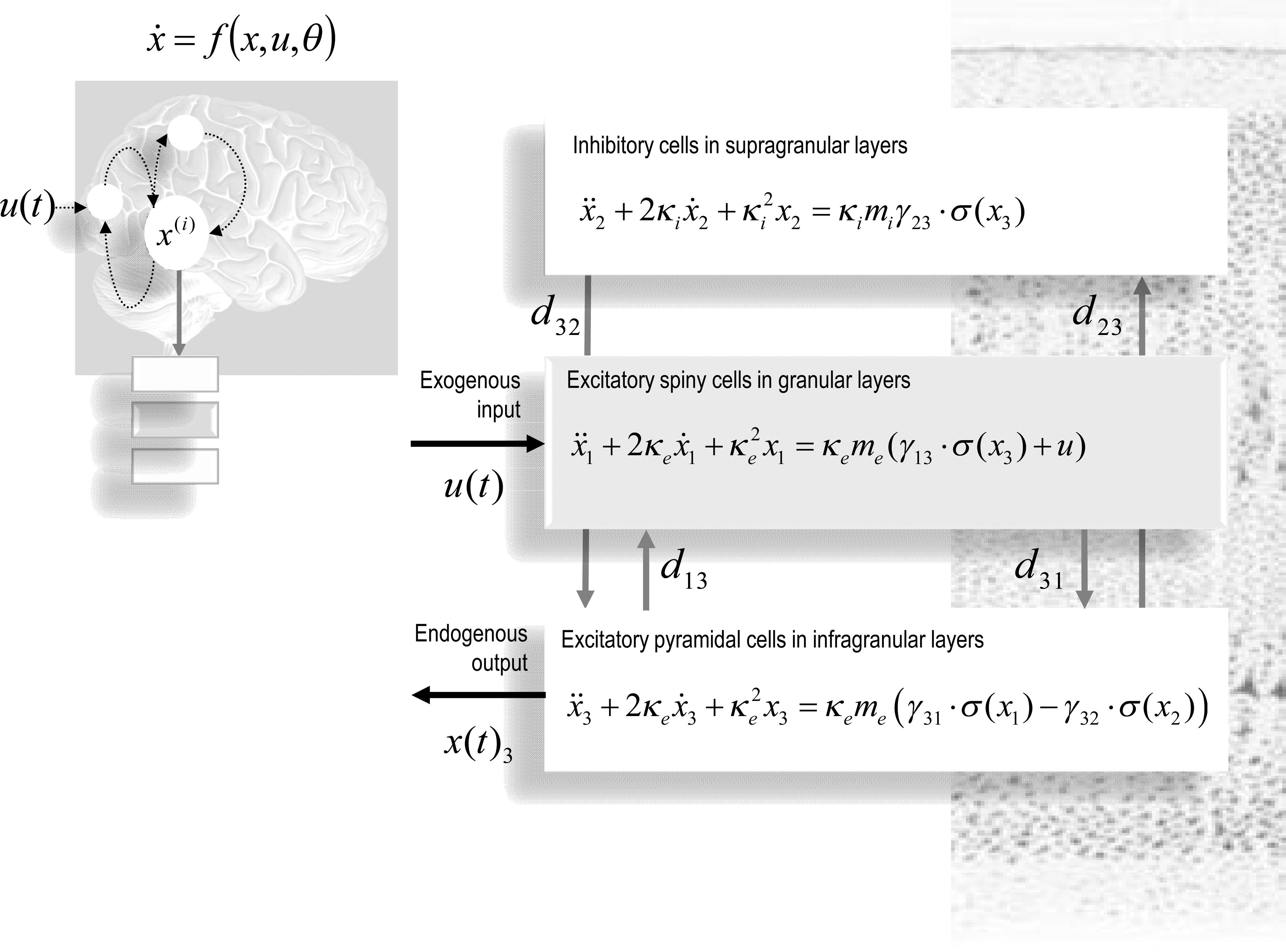
DCM of electromagnetic responses. Neuronally plausible, generative, or forward models are essential for understanding how ERFs and ERPs are generated. DCMs for event-related responses measured with (magneto) electroencephalography use biologically informed models to make inferences about the underlying neuronal networks generating responses. The approach can be regarded as a neurobiologically constrained source reconstruction scheme, in which the parameters of the reconstruction have an explicit neuronal interpretation. Specifically, these parameters encode, among other things, the coupling among sources and how that coupling depends on stimulus attributes or experimental context. The basic idea is to supplement conventional electromagnetic forward models of how sources are expressed in measurement space with a model of how source activity is generated by neuronal dynamics. A single inversion of this extended forward model enables inference about both the spatial deployment of sources and the underlying neuronal architecture generating them. Left panel: This schematic shows a few (three) sources that are coupled with extrinsic connections. Each source is modeled with three subpopulations (pyramidal, spiny-stellate, and inhibitory interneurons). These have been assigned to granular and agranular cortical layers, which receive forward and backward connections, respectively. Right panel: Single-source model with a layered architecture comprising three neuronal subpopulations, each with hidden states describing voltage and conductances for each subpopulation. These neuronal state-equations are based on a Jansen and Rit (1995) model and can include random fluctuations on the neuronal states. The effects of these fluctuations can then be modeled in terms of the dynamics of the ensuing probability distribution over the states of a population; this is known as a mean-field model (Marreiros et al., 2009). ERFs, event-related fields; ERPs, event-related potentials.
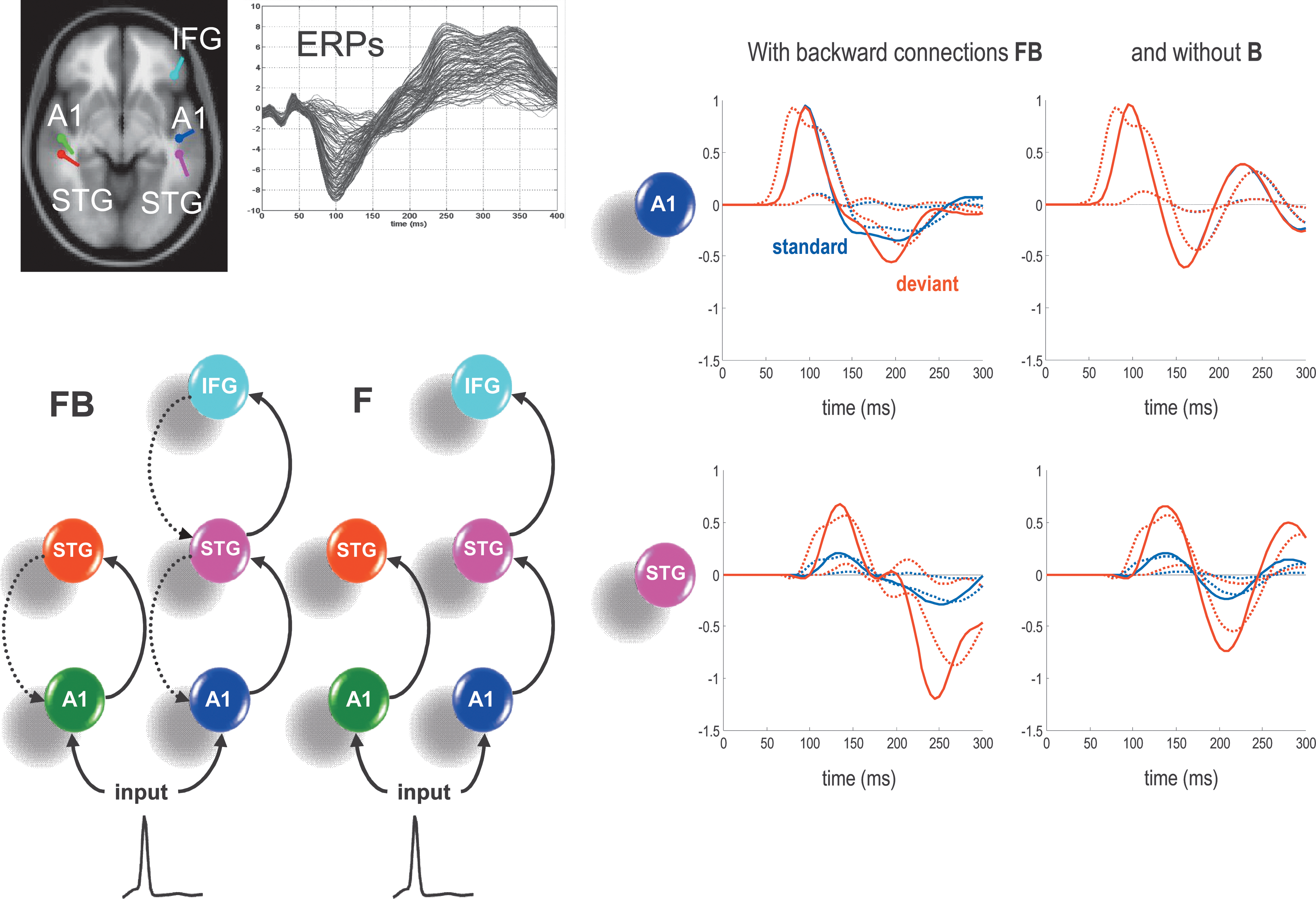
Forward and backward connections (a DCM study of evoked responses). Electrophysiological responses to stimuli unfold over several hundred milliseconds. Early or exogenous components are thought to reflect a perturbation of neuronal dynamics by (bottom-up) sensory inputs. Conversely, later endogenous components have been ascribed to (top-down) recurrent dynamics among hierarchical cortical levels. This example shows that late components of event-related responses are indeed mediated by backward connections. The evidence is furnished by DCM of auditory responses, elicited in an oddball paradigm using electroencephalography. Left (model specification and data): The upper graph shows the ERP responses to a deviant tone, from 0 to 400 ms of peristimulus time (averaged over subjects). Sources comprising the DCM were connected with forward (solid) and backward (broken) connections as shown on the lower left. A1, primary auditory cortex; STG, superior temporal gyrus; IFG, inferior temporal gyrus. Two different models were tested, with and without backward connections (FB and F, respectively). Bayesian model comparison indicated that the best model had forward and backward connections. Sources (estimated posterior moments and locations of equivalent dipoles under the best model) are superimposed on an MRI of a standard brain in MNI space (upper left). Right (hidden neuronal responses): Estimates of hidden states (depolarization in A1 and STG) are shown in the right panels. Dotted lines show the responses of the (excitatory) input population (assigned to the granular layer of cortex), and solid lines show the responses of the (excitatory) output population (assigned to pyramidal cells) (see Fig. 6). One can see a clear difference in responses to standard (blue lines) and deviant (red lines) stimuli, particularly at around 200–300 ms. The graphs on the left show the predicted responses under the full (FB) model, while the right graphs show the equivalent responses after backward connections are removed (B).
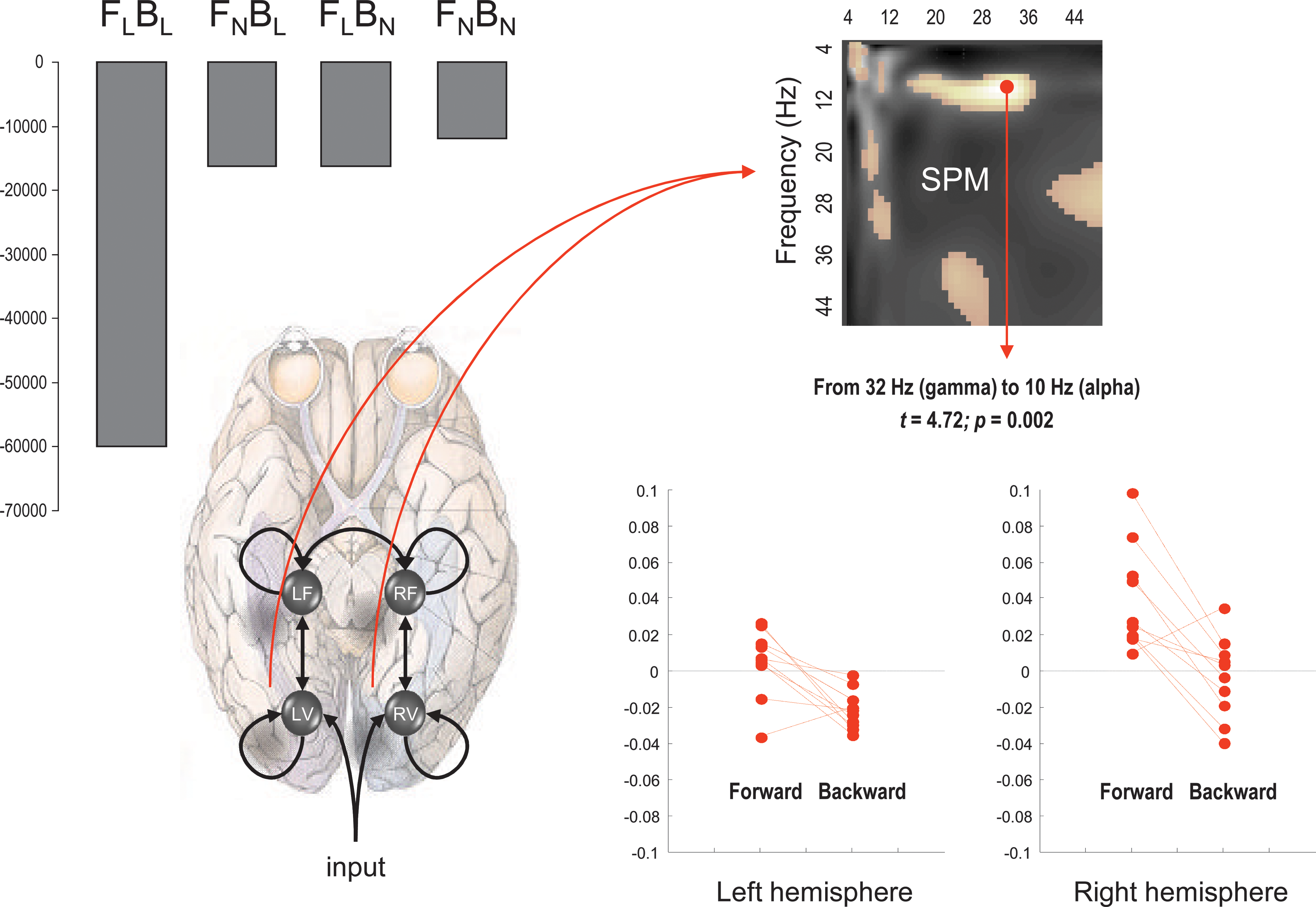
Forward and backward connections (a DCM study of induced responses). This example provides evidence for functional asymmetries between forward and backward connections that define hierarchical architectures in the brain. It exploits the fact that modulatory or nonlinear influences of one neuronal system on another (i.e., effective connectivity) entail coupling between different frequencies. Functional asymmetry is addressed here by comparing dynamic causal models of MEG responses induced by visual processing of faces. Bayesian model comparison indicated that the best model had nonlinear forward and backward connections. Under this model, there is a striking asymmetry between these connections, in which high (gamma) frequencies in lower cortical areas excite low (alpha) frequencies in higher areas, while the reciprocal effect is suppressive. Left panel (upper): Log-evidences (pooled over subjects) for four DCMs with different combinations of linear and nonlinear (N versus L) coupling in forward and backward (F versus B) connections. It can be seen that the best model is FNBN, with nonlinear coupling in both forward and backward connections. Left panel (lower): Location of the four sources (in MNI coordinates) and basic connectivity structure of the models. LV and RV; left and right occipital face area; LF and RF; left and right fusiform face area. Right panel (upper): SPM of the t-statistic (p>0.05 uncorrected) testing for a greater suppressive effect of backward connections, relative to forward connections (over subjects and hemisphere). Right panel (lower): Subject and hemisphere-specific estimates of the coupling strengths at the maximum of the SPM (red arrow). [See Chen et al. (2009) for further details.]
Neural-mass models
More recent efforts have focused on DCMs for electromagnetic (EEG and MEG) data (Chen et al., 2008; Clearwater et al., 2008; David et al., 2006; Garrido et al., 2007a,b, 2008; Kiebel et al., 2006, 2007), with related developments to cover local field potential recordings (Moran et al., 2007, 2008). These models are more sophisticated than the neuronal models for fMRI and are based on neural-mass or mean-field models of interacting neuronal populations (see Deco et al., 2008). Typically, each source of electromagnetic activity is modeled as an equivalent current dipole (or small cortical patch) whose activity reflects the depolarization of three populations (usually one inhibitory and two excitatory). Importantly, one can embed any neural-mass model into DCM. These can include models based on second-order linear differential equations (Jansen and Rit, 1995; Lopes da Silva et al., 1974). Figure 6 shows the general form for these models. As in fMRI, DCM for electromagnetic responses is just a generalization of conventional (equivalent current dipole) models that have been endowed with parameterized connections among and within sources (David et al., 2006). These models fall into the class of spatiotemporal dipole models (Scherg and Von Cramon, 1985) and enable the entire time-series over peristimulus time to inform parameter estimates and model evidence. The construct validity of these models calls on established electrophysiological phenomena and metrics of coupling (e.g., David and Friston, 2003; David et al., 2004). Their predictive validity has been established using paradigms like the mismatch negativity (Näätänen, 2003) as an exemplar sensory learning paradigm (e.g., Garrido et al., 2007b, 2008).
Developments in this area have been rapid and can be summarized along two lines. First, people have explored more realistic neural-mass models based on nonlinear differential equations whose states correspond to voltages and conductances (Morris and Lecar, 1981). This allows one to formulate DCMs in terms of well-characterized synaptic dynamics and to model different types of receptor-mediated currents explicitly. Further, conventional neural-mass modeling (which considers only the average state of a neuronal ensemble) has been extended to cover ensemble dynamics in terms of population densities. This involves modeling not only the average but also the dispersion or covariance among the states of different populations (Marreiros et al., 2009). The second line of development pertains to the particular data features the models try to explain. In conventional DCMs for ERPs, the time course of signals at the sensors is modeled explicitly. However, DCMs for spectral responses (Moran et al., 2007, 2008) can be applied to continuous recordings of arbitrary length. This modeling initiative rests on a linear-systems approach to the underlying neural-mass model to give a predicted spectral response for unknown but parameterized fluctuations. This means that given the spectral profile of electrophysiological recordings one can estimate the coupling among different sources and the spectral energy of neuronal and observation noise generating observed spectra. This has proved particularly useful for local field potentials and has been validated using animal models and psychopharmacological constructs (Moran et al., 2008, 2009). Finally, there are DCMs for induced responses (Chen et al., 2008). Like steady-state models, these predict the spectral density of responses, but in a time-dependent fashion. The underlying neural model here is based on the bilinear approximation above. The key benefit of these models is that one can quantify the evidence for between-frequency coupling among sources, relative to homologous models restricted to within-frequency coupling. Coupling between frequencies corresponds to nonlinear coupling. Being able to detect nonlinear coupling is important because it speaks to the functional asymmetries between forward and backward connections.
Forward and backward connections in the brain
To provide a concrete example of how these developments have been used to build a picture of distributed processing in the brain, we focus on the role of forward and backward message-passing among hierarchically deployed cortical areas (Felleman and Van Essen, 1991). Many current formulations of perceptual inference and learning can be cast in terms of minimizing prediction error (e.g., Ballard et al., 1983; Dayan et al., 1995; Mumford, 1992; Murray et al., 2002; Rao and Ballard, 1998) or, more generally, surprise (Friston et al., 2006). The predictive coding hypothesis‡ suggests that prediction errors are passed forward from lower levels of sensory hierarchies to higher levels to optimize representations in the brain's generative model of its world. Predictions based on these representations are then passed down backward connections to suppress or explain away prediction errors. This message-passing scheme rests on reciprocal or recurrent self-organized dynamics that necessarily involve forward and backward connections. There are some key predictions that arise from this scheme. First, top-down influences mediated by backward connections should have a tangible influence on evoked responses that are modulated by prior expectations induced by priming and attention. Second, the excitatory influences of forward (glutamatergic) connections must be balanced by the (polysynaptic) inhibitory influence of backward connections; this completes the feedback loop suppressing prediction error. Third, backward connections should involve nonlinear or modulatory effects because it is these, and only these, that model nonlinearities in the world that generate sensory input.
These functionally grounded attributes of forward and backward connections, and their asymmetries, are the sorts of things for which DCM was designed to test. A fairly comprehensive picture is now emerging from DCM studies using several modalities and paradigms: Initial studies focused on attentional modulation in visual processing. These studies confirmed that the attentional modulation of visually evoked responses throughout the visual hierarchy could be accounted for by changes in the strength of connections mediated by attentional set (Friston et al., 2003). In other words, no extra input was required to explain attention-related responses; these were explained sufficiently by recurrent dynamics among reciprocally connected areas whose influence on each other increased during attentive states.
More recently, the temporal anatomy of forward and backward influences has been addressed using DCM for ERPs. Garrido et al. (2007a) used Bayesian model comparison to show that the evidence for backward connections was more pronounced in later components of ERPs. Put another way, backward connections are necessary to explain late or endogenous response components in simple auditory ERPs. Garrido et al. (2008) then went on to ask whether one could understand repetition suppression in terms of changes in forward and backward connection strengths that are entailed by predictive coding. DCM showed that repetition suppression, of the sort that might underlie the mismatch negativity (Näätänen, 2003), could be explained purely in terms of a change in forward and backward connections with repeated exposure to a particular stimulus. Further, by using functional forms for the repetition-dependent changes in coupling strength, Garrido et al. (2009) showed that changes in extrinsic (cortico-cortical) coupling were formally distinct from intrinsic (within area) coupling. This was consistent with theoretical predictions about changes in postsynaptic gain with surprise and distinct changes in synaptic efficacy associated with learning under predictive coding.
Figure 7 shows an exemplar analysis using the data reported in Garrido et al. (2008). Data were acquired under a mismatch negativity paradigm using standard and deviant stimuli. ERPs for deviant stimuli are shown as an insert. These data were modeled with a series of equivalent current dipoles (upper left), with connectivity structures shown on the lower left. The architecture with backward (reciprocal) connections among auditory sources had the greatest evidence. The ensuing estimates of hidden states (depolarization in the auditory and superior temporal sources) are shown in the right panels. Dotted lines show the responses of the (excitatory) input population (assigned to the granular layer of cortex), and solid lines show the responses of the (excitatory) output population (assigned to pyramidal cells). One can see a clear difference in responses to standard (blue lines) and deviant (red lines) stimuli, particularly at around 200–300 ms. These differences were modeled in terms of stimulus-specific changes in coupling that can be thought of as mediating sensory learning. The key point illustrated by this figure lies in the rightmost panels. Because analyses of effective connectivity are based on an explicit generative model, one can reconstitute or generate predictions of hidden states (in this example, the activity of hidden dipolar sources on the cortex). Further, one can perform simulated lesion experiments to see what would happen if particular components of the network were removed. This enables one to quantify the contribution of specific connections to regional responses. In Figure 7, we have removed all backward connections, while leaving forward connections unchanged. The resulting responses are shown in the right panels. One obvious effect is that there is now no difference between the responses to standard and deviant stimuli in the primary auditory source. This is because the effects of repetition were restricted to extrinsic connections among sources, and (in the absence of backward connections) these effects cannot be expressed in the sensory source receiving auditory input. More importantly, in the superior temporal source, the late deviant event-related component has now disappeared. It is this component that is usually associated with the mismatch negativity, which suggests that the mismatch negativity per se rests, at least in part, on backward extrinsic connections. This example is presented to illustrate the potential usefulness of biologically grounded generative models to explain empirical data.
Finally, Chen et al. (2009) addressed functional asymmetries in forward and backward connections during face perception, using DCM for induced responses. These asymmetries were expressed in terms of nonlinear or cross-frequency coupling, where high frequencies in a lower area excited low frequencies in a higher area and the reciprocal influences where inhibitory (see Fig. 8). These results may be related to the differential expression of gamma activity in superficial and deep pyramidal cells that are the origin of forward and backward connections, respectively (see Chrobak and Buzsaki, 1998; Fries, 2009; Roopun et al., 2008; Wang et al., 2010). The emerging story here is that forward connections may employ predominantly fast (gamma) frequencies, while backward influences may be meditated by slower (beta) activity.
In conclusion, we have come some way in terms of understanding the functional anatomy of forward and backward connections in the brain. Interestingly, some of the more compelling insights have been obtained by using biophysical models with simple paradigms (like the mismatch negativity) and simple noninvasive techniques (like EEG). All of the examples so far have used evoked or induced responses to make inferences about distributed processing. Can we apply DCM to autonomous or endogenous activity and still find evidence for structured hierarchical processing?
Network discovery
DCM is usually portrayed as a hypothesis-led approach to understanding distributed neuronal architectures underlying observed brain responses (Friston et al., 2003). In general, competing hypotheses are framed in terms of different networks or graphs, and Bayesian model selection is used to quantify the evidence for one network (hypothesis) over another (Penny et al., 2004). However, in recent years, the number of models over which people search (the model-space) has grown enormously—to the extent that DCM is now used to discover the best model over very large model-spaces (e.g., Penny et al., 2010; Stephan et al., 2009). Using DCMs based on random differential equations, it is now possible to take this discovery theme one step further and disregard prior knowledge about the experimental causes of observed responses to make DCM entirely data-led. This enables network discovery using observed responses during both activation studies and (task-free) studies of endogenous activity (Biswal et al., 1995).
This form of network discovery uses Bayesian model selection to identify the sparsity structure (absence of edges or connections) in a dependency graph that best explains observed time-series (Friston et al., 2010). The implicit adjacency matrix specifies the form of the network (e.g., cyclic or acyclic) and its graph-theoretical attributes (e.g., degree distribution). Crucially, this approach can be applied to experimentally evoked responses (activation studies) or endogenous activity in task-free (resting-state) fMRI studies. Unlike structural causal modeling, DCM permits searches over cyclic graphs. Further, it eschews (implausible) Markovian assumptions about the serial independence of random fluctuations. The scheme furnishes a network description of distributed activity in the brain that is optimal in the sense of having the greatest conditional probability (relative to other networks).
To illustrate this approach, Figure 9 shows an example of network discovery following a search over all sparsity structures (combinations of connections), under the constraint that all connections were reciprocal (albeit directional), among six nodes or regions. This example used DCM for fMRI and an attention-to-motion paradigm [see Friston et al. (2010) for details]. Six representative regions were defined as clusters of contiguous voxels surviving an (omnibus) F-test for all effects of interest at p<0.001 (uncorrected) in a conventional statistical parametric mapping (SPM) analysis. These regions were chosen to cover a distributed network (of largely association cortex) in the right hemisphere, from visual cortex to frontal eye fields. The activity of each region (node) was summarized with its principal eigenvariate to ensure an optimum weighting of contributions from each voxel within the region of interest. Figure 9 summarizes the results of post hoc model selection. The upper left panel shows the log-evidence profile over the 32,768 models considered (reflecting all possible combinations of bidirectional edges among the six nodes analyzed). There is a reasonably clear optimum model. This is evident if we plot the implicit log-posterior as a model posterior (assuming flat priors over models), as shown in the upper right panel. In this case, we can be over 80% certain that a specific network generated the observed fMRI data. Parameter estimates of the connections under a model with full connectivity (left) and the selected model (right) are shown in the lower panels. One can see that three (bidirectional) connections have been “switched off.” It is these antiedges that define the architecture we seek. This is a surprisingly dense network, in which all but 3 of the 15 reciprocal connections appear to be necessary to explain observed responses. This dense connectivity may reflect the fact that, in this example, we deliberately chose regions that play an integrative (associational) role in cortical processing (c.f., hubs in graph theory; Bullmore and Sporns, 2009).
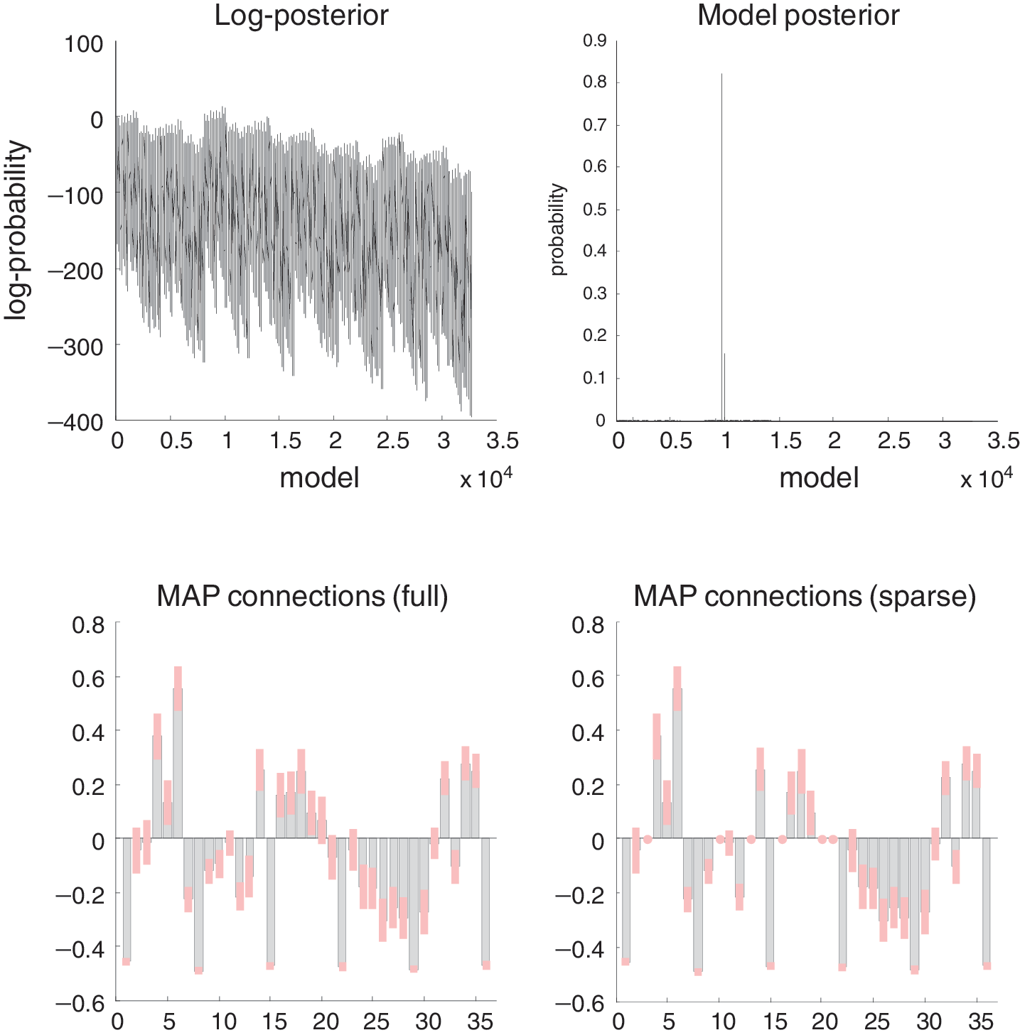
Model selection and network discovery. This figure summarizes the results of model selection using fMRI data. The upper left panel shows the log-evidence profile over all models considered (encoding different combinations of edges among six nodes). The implicit model posterior (assuming flat priors over models) is shown on the upper right and suggests we can be over 80% certain that a particular architecture generated these data. The parameter estimates of the connections under a model with full connectivity (left) and the model selected (right) are shown in the lower panels. We can see that certain connections have been switched off as the parameter estimates are reduced to their prior value of zero. It is these antiedges that define the architecture we are seeking. This architecture is shown graphically in Figure 10.
Figure 10 shows the underlying graph in anatomical and functional (spectral embedding) space. Note that these plots refer to undirected graphs (we will look at directed connection strengths below). The upper panel shows how the six regions are connected using the conditional means of the coupling parameters (in Fig. 9), under the selected (optimal) model. Arrow colors report the source of the strongest bidirectional connection, while arrow width represents absolute (positive or negative) strength. This provides a description of the network in anatomical space. A more functionally intuitive depiction of this graph is provided in the lower panel. Here, we have used spectral embedding to place the nodes in a functional space where the distance between them reflects the strength of bidirectional coupling (this is similar to multidimensional scaling, but uses the graph Laplacian based on the weighted adjacency matrix to define similarities). We conclude by revisiting the issue of forward and backward connections, but here using effective connectivity based on fMRI.
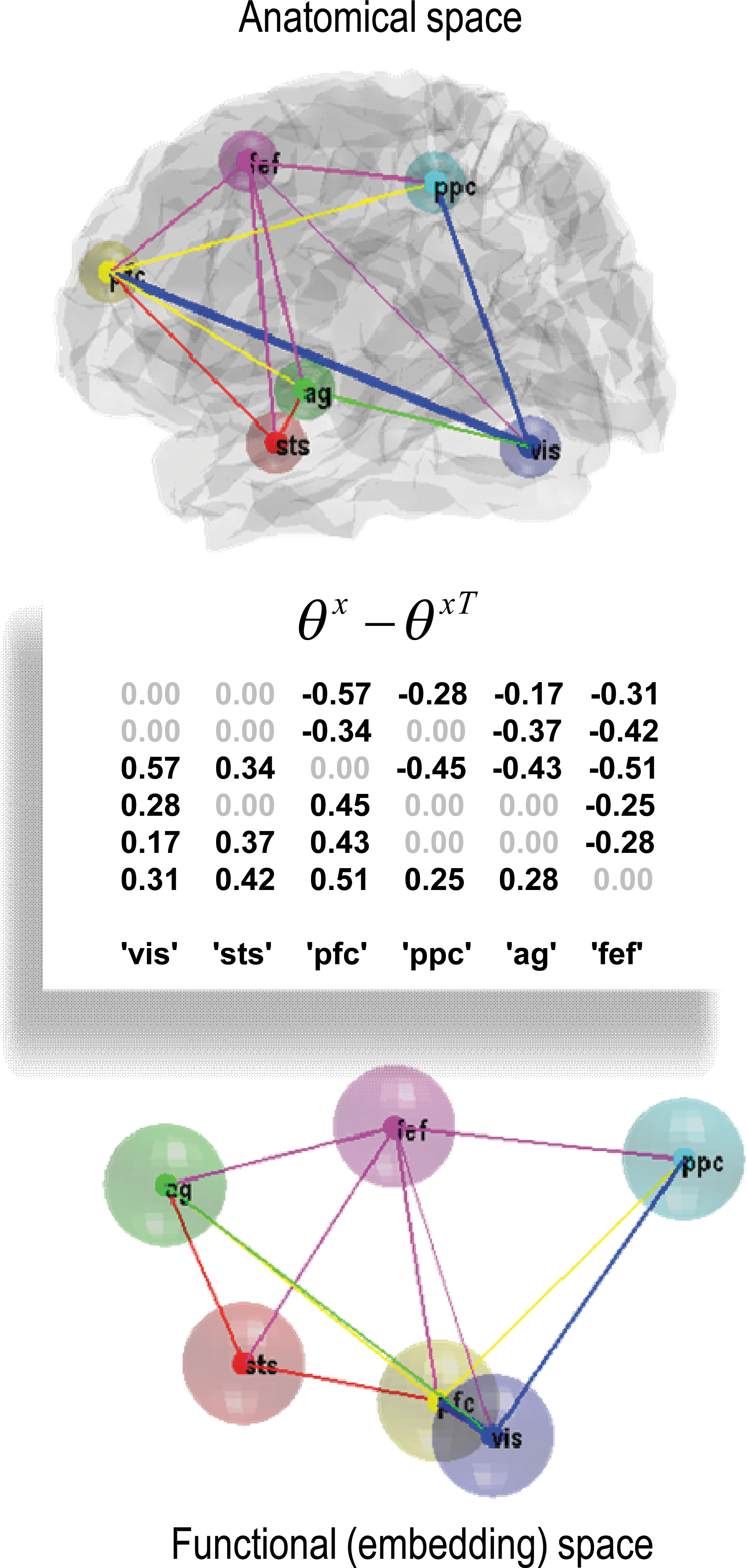
The selected graph (network) in anatomical space and functional space. This figure shows the graph selected (using the posterior probabilities in the previous figure) in anatomical and functional (spectral embedding) space. The upper panel shows the six regions connected, using the conditional means of the coupling parameters (see Fig. 9). The color of the arrow reports the source of the strongest bidirectional connection, while its width represents its absolute (positive or negative) strength. This provides a description of the architecture or graph in anatomical space. A more functionally intuitive depiction of this graph is provided in the lower panel. Here, we have used spectral embedding to place the nodes in a functional space, where the distance between them reflects the strength of bidirectional coupling. Spectral embedding uses the eigenvectors (principal components) of the weighted graph Laplacian to define a small number of dimensions that best captures the proximity or conditional dependence between nodes. Here, we have used the first three eigenvectors to define this functional space. The weighted adjacency matrix was, in this case, simply the maximum (absolute) conditional estimate of the coupling parameters. The middle panel shows the asymmetry in strengths based on conditional estimates. This provides a further way of characterizing the functional architecture in hierarchical terms, based on (bidirectional) coupling.
Asymmetric connections and hierarchies
Network analyses using functional connectivity (correlations among observed neuronal time series) or diffusion-weighted MRI data cannot ask whether a connection is larger in one direction relative to another because they are restricted to the analysis of undirected (simple) graphs. However, here we have the unique opportunity to exploit asymmetries in reciprocal connections and revisit questions about hierarchical organization (e.g., Capalbo et al., 2008; Hilgetag et al., 2000; Lee and Mumford, 2003; Reid et al., 2009). There are several strands of empirical and theoretical evidence to suggest that in comparison to bottom-up influences the net effects of top-down connections on their targets are inhibitory (e.g., by recruitment of local lateral connections; c.f., Angelucci et al., 2003; Crick and Koch, 1998). Theoretically, this is consistent with predictive coding, where top-down predictions suppress prediction errors in lower levels of a hierarchy (see above). One might, therefore, ask which hierarchical ordering of the nodes maximizes the average strength of forward connections relative to their backward homologue. This can be addressed by finding the order of nodes that maximizes the difference between the average forward and backward estimates of effective connectivity. The resulting order was
Summary
In summary, DCM calls on biophysical models of neuronal dynamics by treating them as generative models for empirical time series. The ensuing inferences pertain to the models per se and their parameters (e.g., effective connectivity) that generate observed responses. Using model comparison, one can search over wide model-spaces to find optimal architectures or networks. Having selected the best model (or subset of models), one then has access to the posterior density on the neuronal and coupling parameters defining the network. Of key interest here are changes in coupling that are induced experimentally with, for example, drugs, attentional set, or time. These experimentally induced changes enable one to characterize the context-sensitive reconfiguration of brain networks and test hypotheses about the relative influence of different connections. Recent advances in causal modeling based on random differential equations (Friston et al., 2008) can now accommodate hidden fluctuations in neuronal states that enable the modeling of autonomous or endogenous brain dynamics. Coupled with advances in post hoc model selection, we can now search over vast model-spaces to discover the most likely networks generating both evoked and spontaneous activity. Clearly, there are still many unresolved issues in DCM.
In a discovery context, the specification of the model space is a key issue. In other words, how many and which nodes do we consider? In general, prior beliefs about plausible and implausible architectures determine that space. Usually, these beliefs are implicit in the models considered, which are usually assumed to be a priori equally likely. It should be noted that the posterior probability of a model depends not just on its evidence but on its prior probability. This can be specified quantitatively to moderate the evidence for unlikely models. At present, most DCM considers a rather limited number of nodes or sources (usually up to about eight). A future challenge will be to scale up the size of the networks considered and possibly consider coupling not between regions but between distributed patterns or modes (e.g., Daunizeau et al., 2009).
Conclusion
This review has used a series of (nested) dichotomies to help organize thinking about connectivity in the brain. It started with the distinction between functional segregation and integration. Within functional integration, we considered the key distinction between functional and effective connectivity and their relationship to underlying models of distributed processing. Within effective connectivity, we have looked at structural and dynamic causal modeling, while finally highlighting the distinction between DCM of evoked (induced) responses and autonomous (endogenous) activity.
Clearly, in stepping through these dichotomies, this review has taken a particular path—from functional integration to network discovery with DCM. This has necessarily precluded a proper treatment of many exciting developments in brain connectivity, particularly the use of functional connectivity in resting-state studies to compare cohorts or psychopharmacological manipulations (e.g., Pawela et al., 2008). I am also aware of omitting a full treatment of structure-function relationships in the brain and the potential role of tractography and other approaches to anatomical connectivity. I apologize for this; I have focused on the issues that I am familiar with and believe hold the key to a mechanistic application of connectivity analyses in systems neuroscience. I also apologize if you have been pursuing Granger causality or the comparison of correlations with gay abandon. I have been deliberately contrived in framing some of the conceptual issues to provoke a discussion. I may be wrong about these issues, although I do not usually make mistakes. Having said this, I did make a naive mistake in my first article on functional connectivity (Friston et al., 1993), which no one has subsequently pointed out (perhaps out of kindness). A substantial part of Friston et al. (1993) was devoted to the problem of identifying the eigenvectors of very large (voxel×voxel) matrices, using a recursive (self-calling) algorithm. This was misguided and completely redundant because these eigenvectors can be accessed easily using singular value decomposition of the original (voxel×time) data matrix. I am grateful to Fred Brookstein for pointing this out after seeing me present the original idea. I tell this story to remind myself that every journey of discovery has to begin somewhere, and there is so much to learn (individually and collectively). Given the trends in publications on brain connectivity (Fig. 1), one might guess that we have now embarked on a journey; a journey that I am sure is taking us in the right direction. I would like to conclude by thanking the editors of Brain Connectivity (Chris and Bharat) for asking me to write this review and helping shape its content. On behalf of their readers, I also wish them every success in their editorial undertaking over the years to come.
Footnotes
Acknowledgments
This work was funded by the Wellcome Trust. I would like to thank my colleagues on whose work this commentary is based, including Michael Breakspear, Christian Büchel, C.C. Chen, Jean Daunizeau, Olivier David, Marta Garrido, Lee Harrison, Martin Havlicek, Maria Joao, Stefan Kiebel, Baojuan Li, Andre Marreiros, Andreas Mechelli, Rosalyn Moran, Will Penny, Alard Roebroeck, Olaf Sporns, Klaas Stephan, Pedro Valdés-Sosa, and many others. I thank Klaas Stephan in particular for reading this article carefully and advising on its content.
Author Disclosure Statement
No competing financial interests exist.
*
Strictly speaking, the center manifold theorem is used to reduce the degrees of freedom only in the neighborhood of a bifurcation.
†
In other words, we assume that neural dynamics are an adiabatic process that adapts quickly to slowly fluctuating perturbations.
‡
Predictive coding refers to an estimation or inference scheme (developed originally in engineering) that has become a popular metaphor for neuronal inference and message-passing in the brain.