Sample Size Estimation for Comparing Parameters Using Dynamic Causal Modeling

Abstract

Functional magnetic resonance imaging (fMRI) has proved to be useful for analyzing the effects of illness and pharmacological agents on brain activation. Many fMRI studies now incorporate effective connectivity analyses on data to assess the networks recruited during task performance. The assessment of the sample size that is necessary for carrying out such calculations would be useful if these techniques are to be confidently applied. Here, we present a method of estimating the sample size that is required for a study to have sufficient power. Our approach uses Bayesian Model Selection to find a best fitting model and then uses a bootstrapping technique to provide an estimate of the parameter variance. As illustrative examples, we apply this technique to two different tasks and show that for our data, ∼20 volunteers per group is sufficient. Due to variability between task, volunteers, scanner, and acquisition parameters, this would need to be evaluated on individual datasets. This approach will be a useful guide for Dynamic Causal Modeling studies.

Introduction

I maging studies, including functional magnetic resonance imaging (fMRI), have shown that the brain areas recruited while carrying out a cognitive task do not work in isolation, and that instead a network of brain areas is recruited (Frackowiack et al., 2004). Defined as “the influence of one brain region on another,” effective connectivity makes it possible to test the networks of brain regions to find the mechanism contributing to changes in cognitive activations. A recently established method that assesses effective connectivity is dynamic causal modeling (DCM) (Friston et al., 2003). Using DCM, effective connectivity is characterized by “intrinsic connections” that specify which regions are connected and denote the connectivity in the absence of task activation. Inputs are also defined, which dictate the perturbation of the system and which areas these influence. Finally, modulatory connections are specified, which dictate which connections may be changed by a factor of the task performed.

Effective connectivity studies using DCM may contribute valuable information regarding the neurobiological mechanisms of psychiatric illnesses (Rowe et al., 2010; Sonty et al., 2007) and psychoactive drug action (Stephan et al., 2007). Before embarking on such studies, it is important to estimate the number of volunteers required for a study to observe the effect of interest. Horwitz (2003) argues that it may be difficult to make inferences from effective connectivity analyses due to variability, arising from volunteers using different strategies for completing tasks and researchers having different hypotheses and specifying different models. Therefore, studies investigating the variability of effective connectivity results are needed. A DCM study using EEG data was carried out by Garrido et al. (2007), who found that Bayesian Model Selection (BMS) chose the same model consistently; however, the variability in the individual parameters was not investigated. A study by Rowe et al. (2010) found DCM and BMS to be reliable and reproducible for the study of Parkinson's disease. Our previous work has shown that nonparametric permutation tests provide more power for testing for between-group differences compared with the parametric equivalent (Goulden et al., 2010).

There are two possible approaches to performing a DCM study comparing two groups (Stephan et al., 2010). The first approach is to use BMS (Penny et al., 2004, 2010; Stephan et al., 2009a) to find a separate best-fitting model for each group, focusing more on the model structure and how it differs between groups. A second approach is to use BMS in both groups together to find a single best-fitting model and then compare parameter values. This article presents a method for estimating the sample size (SS) for a study when the intention is to compare parameter values.

SS estimation has been previously carried out for fMRI studies. A study conducted by Desmond and Glover (Desmond and Glover, 2002) found that for typical activation tasks, 12 volunteers are required to achieve 80% power at a single voxel level of p<0.05 uncorrected. The number of volunteers required when correcting for multiple comparisons doubled to 24.

As illustrative examples, we perform SS estimation for DCM analyses of data from two cognitive tasks, an implicit face emotion processing task previously used by our group to investigate drug effects and the differences between psychiatric groups (Anderson et al., 2007, 2010; Del-Ben et al., 2005) and an n-back task (Honey et al., 2002; Owen et al., 2005; Schlosser et al., 2006).

We employ a bootstrapping procedure that estimates the population variance. Bootstrapping has been previously used in the context of fMRI for activation detection (Darki and Oghabian, 2009) and to assess the stability of resting-state clusters (Bellec et al., 2010).

The implicit face emotion processing task has been used to identify the brain regions associated with face and emotion processing. The brain areas found to be important for face emotion processing include the fusiform gyrus (FG), amygdale, and lateral orbitofrontal cortex (LOFC) (Phan et al., 2002). Tractography studies have also demonstrated white matter tracts between these regions (Cavada et al., 2000; Ghashghaei and Barbas, 2002; Iidaka et al., 2001), making them good candidate regions for an effective connectivity analysis.

The N-back task is generally used to identify the brain regions associated with the working memory. The dorsolateral prefrontal cortex (DPC) is critically involved in this task (Callicott et al., 1999), together with superior frontal areas, including the supplementary motor area (SMA) (Cohen et al., 1997) and the posterior parietal cortex (PPC) (Callicott et al., 1999). Tractography studies have shown white matter tracts between the parietal cortex and SMA (Petrides and Pandya, 1984), parietal cortex and frontal cortex (Petrides and Pandya, 1984), and SMA and frontal cortex (Bates and Goldman-Rakic, 1993; McGuire et al., 1991).

In this study, we initially applied BMS to a number of DCMs and then applied a bootstrapping analysis to the DCM parameters from the selected model in order to estimate the population standard deviation of the parameters of DCM.

Materials and Methods

Volunteers

Twenty-four right-handed volunteers (12 men) aged 18–23 were recruited by local advertisements. This SS has previously been shown to be adequate (Desmond and Glover, 2002) for achieving 80% power at the single voxel level for typical corrected fMRI activations. The local ethics committee approved the study, and each volunteer provided written informed consent before participating. Volunteers had no personal or family history of psychiatric illness and no contraindications to MR scanning.

Implicit face emotion processing task

A series of faces were presented to the volunteers, with an equal number of male and female faces. Emotional faces were presented for 3 sec with a 1 sec gap. There were three blocks of five face stimuli presented (neutral [N], anger [A], and fear [F]) and a rest (R) block where a fixation cross was displayed. Each block was 20 sec long and was shown in NANRNFNRNANRNFNRNANRNFNR order. The total duration of the task was, therefore, 8 min. At each presentation of a face, the volunteers responded with a button press to indicate whether they perceived the face on the screen to be that of a man or a woman; they were not told of any change in the emotion of the faces and were not asked to attend to the faces' emotion.

n-back task

Each block of this task consisted of a series of 13 letters. Each letter was presented for 1.5 sec with a 0.5 sec interval. At the beginning of each block, an instruction screen stated when the subject was to press a button within that block. There were three task blocks: 0-back (Press on appearance of the letter X), 1-back (Press when the letter presented is the same as the previous one), and 2-back (Press when the letter presented is the same as the one before last). There was also a rest block (R) where a fixation cross was presented for the same length of time as the active blocks. Each block was 26 sec long with 9 sec for the instruction screen for each active block with the rest block lasting for 35 sec. The blocks were presented in 01R02R02R01R02R01R order. The total length of the task was 10 min.

Functional magnetic resonance imaging

Images were acquired using a single-shot echo-planar pulse sequence on a 1.5T Phillips Intera scanner (Eindhoven, Netherlands) housed in the Wellcome Trust Clinical Research Facility, University of Manchester, United Kingdom. Each three-dimensional volume comprised 29 contiguous axial slices (repetition time [TR]/echo time [TE]=2100/40 ms, 3.5 mm by 3.5 mm in-plane resolution, slice thickness 4.5 mm with a 0.5 mm gap). A high-resolution T1-weighted structural image was also collected for each volunteer to assist with registration to standard stereotactic space. For the implicit face recognition task, 227 volumes were acquired, while for the n-back task, 285 volumes were acquired. No volumes were discarded before analysis, as the Philips scanner automatically excluded T1 magnetization equilibrium volumes.

Image analysis

All preprocessing was carried out in SPM5 (www.fil.ion.ucl.ac.uk/spm). Images were slice timing corrected and then realigned to the first volume to correct for volunteer movement in the scanner. The anatomical image was co-registered to the mean functional image, and then, the anatomical image was segmented into gray matter, white matter, and CSF. The functional images were normalized to the anatomical image and smoothed with a three-dimensional Gaussian kernel with full width at a half maximum of 7 mm by 7 mm by 10 mm, twice the voxel size collected. A high-pass filter equal to twice the stimulus repetition time (320 sec for the implicit face recognition task and 210 sec for the n-back task) was applied.

The task regressors included in the general linear model comprised all task-active blocks. For the implicit face recognition task, this included blocks of neutral faces, fearful faces, and angry faces. For the n-back task, this included blocks of 0-, 1-, and 2-back, and the time taken to read the instructions at the start of each block. The second task regressor modeled the condition we were interested in for testing modulations for fearful faces and 2-back, respectively. Motion parameters were included as covariates of no interest in the first-level analysis. A random-effects one-sample t-test was carried out for each task in order to identify the activations that were significant across the entire group of volunteers. Data were extracted, and adjusted for effects of interest, from regions of interest defined using the fearful face and 2-back contrasts, respectively.

Dynamic causal modeling

DCM8 analysis was performed using SPM8. For each individual, local maxima were found within 14 mm of the most significant group activation in the prehypothesized areas for each task, using a threshold of p<0.05 uncorrected. Data were then extracted from a 6 mm radius sphere region of interest. The DCM models were specified for brain regions from the right hemisphere only using the toolbox in SPM8. Random effects (BMS) (Stephan et al., 2009a) was used to determine the best intrinsic connectivity model for each task. This approach computes an expected probability and an exceedance probability, the probability that a model is a better fit than any other model in the model space. The intrinsic connectivity models tested for the implicit face emotion processing task and n-back task are shown in Figures 1a and 2a. These models were tested to reveal whether there are feed-forward or reciprocal connections between regions and whether the input region is connected to the most anterior region in the model (OFC and DPC for implicit face recognition and n-back tasks, respectively). In order to assess whether the results were related to model structure, in particular the origin of the input, the n-back task models were tested with the input going into the PPC dotted in Figure 2a and then separately with the input into the DPC. We display the eight intrinsic models tested for simplicity; these models were tested with input into the PPC (labeled models 1–8) and input into the DPC (labeled models 9–16). For the implicit face recognition task, the fully connected intrinsic model, Figure 3a, was the best fit (exceedance probability 0.2822, Figure 1b, where the top plot shows the expected probability, and the bottom plot indicates the exceedance probability). For the n-back task, the fully connected intrinsic model with input entering the DPC, Figure 3b was the best fit (exceedance probability 0.5220, Figure 2b). Models with modulations by fearful faces and 2-back were then tested, using the optimum intrinsic connectivity models for the implicit face emotion processing task and n-back task, respectively. These models are shown in Figure 3c. First, we tested for the possibility that a single feed-forward connection was modulated by an emotion, then all possible pairs of feed-forward connections, and finally, all feed-forward connections. Feed-back connections were then tested in the same way. Finally, we tested reciprocal connection modulations (feed-forward and feed-back), first between one pair of brain regions, then between two pairs of brain regions followed by every connection being modulated.

FIG. 1.

(a) The intrinsic models tested for the implicit face emotion processing task. Faces versus rest was used as input to the fusiform gyrus (FG). Other areas included in the model are the amygdala (A) and lateral orbitofrontal cortex (LOFC). (b) Results of Bayesian Model Selection for implicit face emotion processing.

FIG. 2.

(a) The intrinsic models tested for the n-back task. N-back versus rest was used as input. Inputs were tested separately entering the posterior parietal cortex (PPC) (solid line) (models 1 to 8 with PPC input) or dorsolateral prefrontal cortex (DPC) (dashed line) (models 1 to 8 with DLPFC input, referred to as models 9 to 16). (b) Results of Bayesian Model Selection for the n-back task. SMA, supplementary motor area.

FIG. 3.

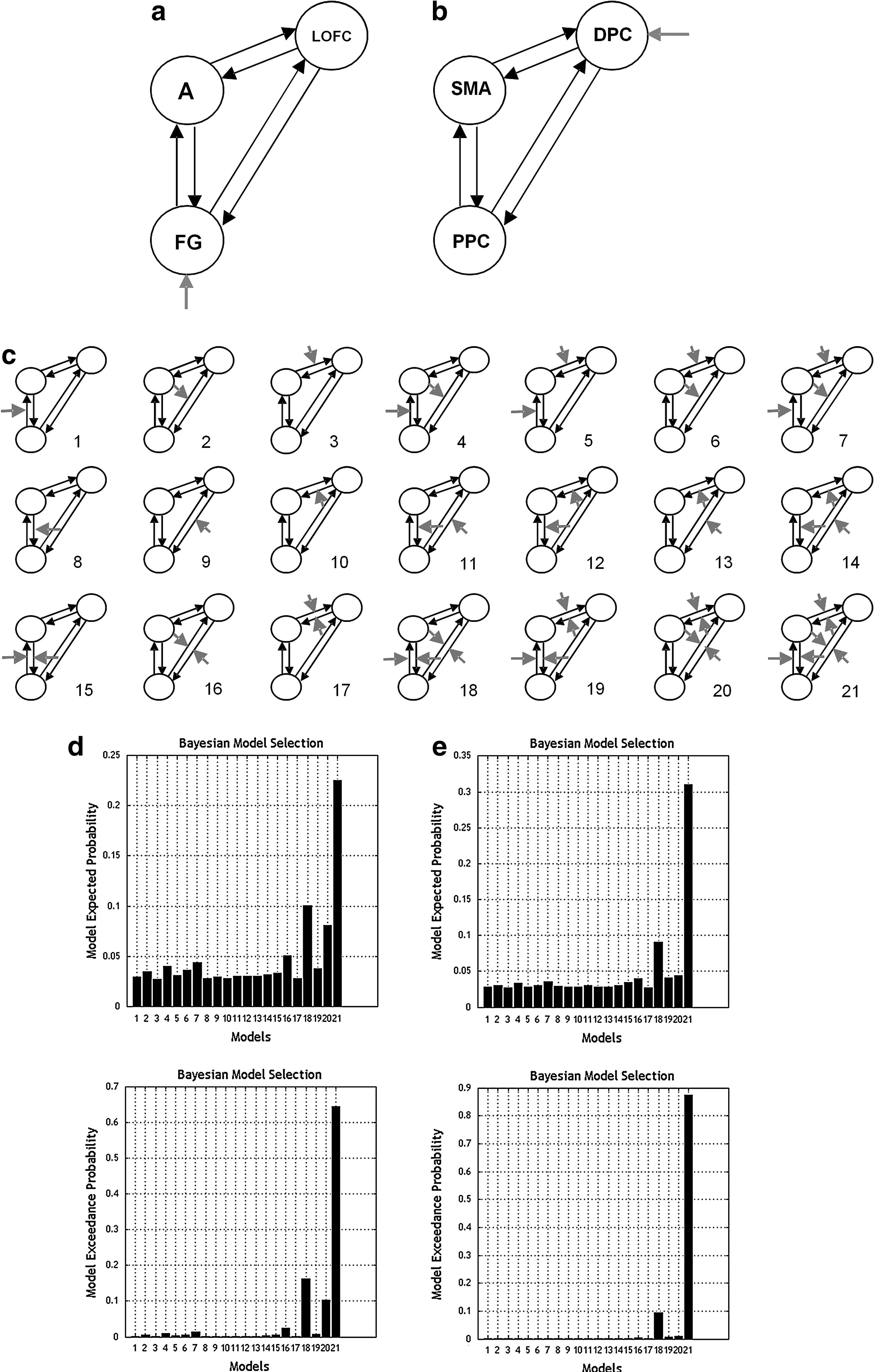
Models for the implicit face emotion processing and n-back tasks. (a) The optimum intrinsic connectivity tested for the implicit face motion processing task. Faces versus rest was used as input to the FG. Other areas included in the model are the amygdala (A) and LOFC. (b) The optimum intrinsic connectivity tested for the n-back task. N-back versus rest was used as input to the DLPFC. The other area included in the model is the SMA. (c) The modulatory models tested for modulations by fearful faces for the implicit face emotion processing task and 2-back for the n-back task. Results for models included modulatory terms (right) for faces (d) and N-back (e) tasks.

Bootstrapping inference

Bootstrapping involves sampling with replacement from the original data to construct the distribution of results under the null hypothesis (Good, 2005). We are interested in a two-sample t-test, so random groups are generated, which are of equal size to the groups in our data (i.e., 17 and 22 for n-back and face processing respectively—the size of each group is explained in the results section). The mean was calculated for each of the random groups we generated. This distribution was then used to obtain an estimate of the population standard deviation (s) for each DCM parameter (i.e., calculating the standard deviation of the generated distribution). The bootstrapped distribution of each parameter was also tested for normality using the Kolmogorov–Smirnov test.

The SS necessary to observe a significant difference between the means of two groups of size d may be estimated, using Equation 1 (Dell et al., 2002). This equation is specific to a two-sample t-test and provides the SS per group for achieving 80% power at a significance level of 0.05. A typical difference between means was obtained from two previous effective connectivity studies: phonological processing in children with and without reading difficulties (Cao et al., 2008) and in healthy controls and patients with primary progressive aphasia (Sonty et al., 2007). The models specified had three and six regions, respectively. A typical significant difference between the means of groups was 0.03. In this study, 0.05 was also used as a less stringent test for a larger group difference.

The following section provides the derivation of Equation 1 (Dell et al., 2002), from Snedecor and Cochran (Snedecor and Cochran, 1989). This equation is used to estimate the necessary SS per group. It is important to bear in mind that the SS found using this equation needs to be doubled. \documentclass{aastex}\usepackage{amsbsy}\usepackage{amsfonts}\usepackage{amssymb}\usepackage{bm}\usepackage{mathrsfs}\usepackage{pifont}\usepackage{stmaryrd}\usepackage{textcomp}\usepackage{portland, xspace}\usepackage{amsmath, amsxtra}\pagestyle{empty}\DeclareMathSizes{10}{9}{7}{6}\begin{document}\begin{align*}SS = \frac { 15.8 s^2 } { d^2 } + 1 \tag { 1 } \end{align*}\end{document}

Equation 1: The relationship between effect size (d), standard deviation (s) of the bootstrap distribution, and SS

In order to use Equation 1, the experimenter needs to supply the value of d (the size of the difference of interest), the desired probability, P′, of obtaining a significant result if the true difference is d, and the significance level of the test, α. Assume that the standard deviation, s, is known, and s_Group1=s_Group2=s. The power of a two-tailed test of H₀: μ=μ₀ (null hypothesis of equal means) against H_A: μ=μ_A (alternative hypothesis of nonequal means) is the probability that the normal deviate Z lies in one of the regions, that is, \documentclass{aastex}\usepackage{amsbsy}\usepackage{amsfonts}\usepackage{amssymb}\usepackage{bm}\usepackage{mathrsfs}\usepackage{pifont}\usepackage{stmaryrd}\usepackage{textcomp}\usepackage{portland, xspace}\usepackage{amsmath, amsxtra}\pagestyle{empty}\DeclareMathSizes{10}{9}{7}{6}\begin{document}\begin{align*}Z < \left( \frac { - \sqrt { n } } { s } \right) ( \mu_A - \mu_0 ) - Z_ { \alpha } \ { \rm or } \ Z > \left( \frac { - \sqrt { n } } { s } \right) ( \mu_A - \mu_0 ) + Z_ { \alpha } \end{align*}\end{document}

where Z _α denotes the two-tailed significance level. In this case, H₀ =μ₀=0 and H_A=μ_A=δ, assumed >0.

The test criterion for the independent samples t-test is \documentclass{aastex}\usepackage{amsbsy}\usepackage{amsfonts}\usepackage{amssymb}\usepackage{bm}\usepackage{mathrsfs}\usepackage{pifont}\usepackage{stmaryrd}\usepackage{textcomp}\usepackage{portland, xspace}\usepackage{amsmath, amsxtra}\pagestyle{empty}\DeclareMathSizes{10}{9}{7}{6}\begin{document}$$\sqrt{n} ( \overline{X}_1 - \overline{X}_2 ) / ( \sqrt{2}s )$$\end{document} . Therefore, \documentclass{aastex}\usepackage{amsbsy}\usepackage{amsfonts}\usepackage{amssymb}\usepackage{bm}\usepackage{mathrsfs}\usepackage{pifont}\usepackage{stmaryrd}\usepackage{textcomp}\usepackage{portland, xspace}\usepackage{amsmath, amsxtra}\pagestyle{empty}\DeclareMathSizes{10}{9}{7}{6}\begin{document}\begin{align*}Z < \frac { - \sqrt { n } d } { \sqrt { 2 } s } - Z_ { \alpha } \ { \rm or } \ Z > \frac { - \sqrt { n } d } { \sqrt { 2 } s } + Z_ { \alpha } \end{align*}\end{document}

Since we want 80% power for the two-tailed test at a 5% significance level, we use Z0.05=1.96. We also need the value for the normal deviate that is exceeded by 80% of the distribution, which is Z=−0.842. Therefore, \documentclass{aastex}\usepackage{amsbsy}\usepackage{amsfonts}\usepackage{amssymb}\usepackage{bm}\usepackage{mathrsfs}\usepackage{pifont}\usepackage{stmaryrd}\usepackage{textcomp}\usepackage{portland, xspace}\usepackage{amsmath, amsxtra}\pagestyle{empty}\DeclareMathSizes{10}{9}{7}{6}\begin{document}\begin{align*} & - 0.842 = \frac { - \sqrt { n } d } { \sqrt { 2 } s } + 1.96 \\ & \frac { \sqrt { n } d } { \sqrt { 2 } s } = 2.802 \\ & n = \frac { 15.8s^2 } { d^2 } \end{align*}\end{document}

The bootstrapping procedure was used to generate 5000 resamples. The entire bootstrapping procedure (i.e., generating 5000 bootstrap resamples) was repeated 1000 times, generating 1000 bootstrap distributions and thereby generating a distribution of SS estimates in order to calculate confidence intervals. The mean of this SS distribution as well as the 95% confidence intervals was calculated, by taking the values for the top and bottom 2.5% of the distribution.

We also assessed the size of the difference between means that could be declared as significant with these data by using Equation 1.

Results

Demographical and behavioral measures

Volunteers were 12 men, mean age 20.25 years (standard deviation [SD] 1.66) and 12 women, mean age 20.08 years (SD 1.56). The mean IQ score for men was 92.92 (SD 8.23), and the mean IQ score for women was 92.67 (SD 6.46). One male volunteer was found to have an IQ of 69 based on the Quick test (>2.5 standard deviations below the mean) and was excluded from subsequent analysis.

Implicit face emotion processing task

Behavioral data

The mean accuracy in the task was 86.6% correct gender identification, and the mean reaction time for classifying the gender of the face was 1254 ms (SD 427.2 ms).

fMRI group activation

Statistically significant voxel level activations were found in the three regions of interest on the right in the fear versus rest contrast at the group level: FG (MNI coords=39, −56, −15; T=8.19, p(FWE)<0.001), amygdala (MNI=25, −7, −20; T=6.68, p(FWE)=0.012), and LOFC (MNI=56, 25, 0; T=5.18, p(FWE)=0.229, p(FWE=0.005 small volume corrected using the WFU PickAtlas mask of the inferior frontal gyrus which contained 611 voxels).

DCM and bootstrapping

Significant amygdala activity was not detected, using a significance level of p<0.05 uncorrected, in 6 volunteers; therefore, the DCM and bootstrap analysis was carried out on data obtained from the remaining 17 volunteers. The best-fitting model found using BMS was model 21 from Figure 3c, and the BMS results are shown in Figure 3d. The exceedance probability for this model was far larger than that for any of the other models (0.6651), making this model the best-fitting model from the model space tested. All the parameter values from the 17 subjects are normally distributed, as shown by the results of a 1-sample Kolmogorov–Smirnov test depicted in Table 1. The SS estimates per group, which need to be doubled for a two-sample t-test, including confidence intervals, are detailed in Table 2, along with the means and standard deviations of the bootstrapping distributions. Examples of the bootstrapping distribution with 5000 resamples are shown in Figure 4 for intrinsic connections emanating from the input regions and not emanating from the input regions, along with the distributions of SS estimates. The SS estimates in Table 2 show that 20 volunteers per group would allow the detection of a significant difference between groups of 0.03, and 8 volunteers would allow the detection of a significant difference between groups of 0.05 in 9 out of the 12 parameters. Correcting for the number of subjects who did not show any amygdala activation makes these numbers 27 for d=0.03 and 11 for d=0.05. The confidence intervals in the SS estimates are small, indicating that these are robust results for these data.

FIG. 4.

An example of the bootstrap distribution from the face emotion recognition task obtained with 5000 resamples for an intrinsic connection from FG to OFC (a) and amygdala to OFC (b), along with the distributions of sample size estimates for the same two connections, (c) and (d) respectively.

Table 1.

Results of the Kolmogorov–Smirnov Test of Normality of the Distribution of the Parameter Values for the Implicit Face Emotion Processing Task (Top Half of Table) and n-Back Task (Bottom Half of Table)

Faces
Connection	FG→Amyg	FG→LOFC	Amyg→FG	Amyg→LOFC	LOFC→FG	LOFC→Amyg
Intrinsic
1-sample KS p-value	0.430	0.181	0.918	0.703	0.995	0.835
Modulations
1-sample KS p-value	0.297	0.312	0.101	0.785	0.425	0.104

n-back
Connection	PPC→SMA	PPC→DPC	SMA→PPC	SMA→DPC	DPC→PPC	DPC→SMA
Intrinsic
1-sample KS p-value	0.575	0.910	0.966	0.945	1.000	0.494
Modulations
1-sample KS p-value	0.955	0.948	0.818	0.688	0.713	0.731

All parameters fit a normal distribution.

Amyg, Amygdala; FG, fusiform gyrus; DPC, dorsolateral prefrontal cortex; KS, Kolmogorov-Smirnov; LOFC, lateral orbitofrontal cortex; PPC, posterior parietal cortex; SMA, supplementary motor area.

Table 2.

The Mean of All the Bootstrap Resamples and Standard Deviation Together with Mean and Confidence Intervals of Sample Size Estimates Per Group at Two Different Effect Sizes for Intrinsic Connections and Modulations

Faces
Connection	FG→Amyg	FG→LOFC	Amyg→FG	Amyg→LOFC	LOFC→FG	LOFC→Amyg
Intrinsic
Mean of all bootstrap (mean SD)	0.0843 (0.1193)	0.1871 (0.2872)	0.1470 (0.0557)	0.1716 (0.1287)	0.2176 (0.0720)	0.1399 (0.1150)
Mean SS, d=0.03 [95% CI]	16.3 [15.7, 16.9]	89.1 [85.8, 92.3]	4.3 [4.2, 4.5]	19.0 [18.2, 19.6]	7.1 [6.8, 7.3]	16.2 [15.6, 16.8]
Mean SS, d=0.05 [95% CI]	6.5 [6.3, 6.7]	32.7 [31.5, 33.9]	2.2 [2.15, 2.24]	7.5 [7.2, 7.7]	3.2 [3.1, 3.3]	6.5 [6.2, 6.7]
Difference between means [95% CI]	0.0294 [0.0288, 0.0299]	0.0687 [0.0674, 0.0699]	0.0151 [0.0149, 0.0154]	0.0317 [0.0310, 0.0322]	0.0193 [0.0190, 0.0197]	0.0293 [0.0287, 0.0298]
Modulations
Mean of all Bootstrap (mean SD)	0.1167 (0.1555)	0.2203 (0.2233)	0.1501 (0.0710)	0.1452 (0.1041)	0.2157 (0.0637)	0.1251 (0.0966)
Mean SS, d=0.03 [95% CI]	28.0 [26.9, 29.0]	56.2 [54.0, 58.5]	6.4 [6.2, 6.6]	13.1 [12.6, 13.6]	5.4 [5.2, 5.5]	11.6 [11.2, 12.1]
Mean SS, d=0.05 [95% CI]	10.7 [10.3, 11.1]	20.9 [20.1, 21.7]	3.0 [2.9, 3.0]	5.4 [5.2, 5.5]	2.6 [2.5, 2.6]	4.8 [4.7, 5.0]
Difference between means [95% CI]	0.0385 [0.0378, 0.0392]	0.0546 [0.0535, 0.0557]	0.0184 [0.0181, 0.0187]	0.0264 [0.0259, 0.0269]	0.0169 [0.0166, 0.0171]	0.0248 [0.0243, 0.0253]

n-back
Connection	PPC→SMA	PPC→DPC	SMA→PPC	SMA→DPC	DPC→PPC	DPC→SMA
Intrinsic
Mean of all Bootstrap (mean SD)	0.2085 (0.1480)	0.1645 (0.1084)	0.2218 (0.1757)	0.1460 (0.1104)	0.2544 (0.1897)	0.2562 (0.2472)
Mean SS, d=0.03 [95% CI]	19.1 [17.5, 20.6]	10.8 [10.0, 11.7]	27.2 [24.8, 29.5]	11.3 [10.4, 12.2]	30.5 [28.0, 33.0]	51.3 [47.4, 55.5]
Mean SS, d=0.05 [95% CI]	7.5 [6.9, 8.1]	4.5 [4.2, 4.9]	10.4 [9.6, 11.2]	4.7 [4.4, 5.0]	11.6 [10.7, 12.5]	19.1 [17.7, 20.6]
Difference between means [95% CI]	0.0286 [0.0274, 0.0297]	0.0215 [0.0207, 0.0224]	0.0341 [0.0326, 0.0355]	0.0220 [0.0211, 0.0229]	0.0361 [0.0346, 0.0376]	0.0469 [0.0451, 0.0488]
Modulations
Mean of all Bootstrap (mean SD)	0.0956 (0.1113)	0.1504 (0.1140)	0.1330 (0.1249)	0.1418 (0.0966)	0.2233 (0.2170)	0.1728 (0.1854)
Mean SS, d=0.03 [95% CI]	11.4 [10.5, 12.3]	11.7 [10.8, 12.6]	14.5 [13.3, 15.8]	8.8 [8.1, 9.4]	41.4 [38.0, 45.2]	30.5 [28.0, 33.2]
Mean SS, d=0.05 [95% CI]	4.7 [4.4, 5.1]	4.8 [4.5, 5.2]	5.9 [5.4, 6.3]	3.8 [3.6, 4.0]	15.5 [14.3, 16.9]	11.6 [10.7, 12.6]
Difference between means [95% CI]	0.0221 [0.0212, 0.0230]	0.0223 [0.0215, 0.0232]	0.0250 [0.0239, 0.0260]	0.0194 [0.0186, 0.0201]	0.0421 [0.0403, 0.0440]	0.0361 [0.0347, 0.0377]

We also include estimates of the difference between means that could be detected as significant.

CI, confidence intervals; SD, standard deviation; SS, sample size.

The SS values of FG→Amyg and FG→OFC connections and modulations are generally larger than those for the rest of the parameters. By excluding these connections and modulations, the average SS value reduced from 22.7 (25.3) to 10.4 (5.4) for d=0.03 and from 8.8 (9.1) to 4.4 (2.0) for d=0.05.

For the majority of parameters, the difference between means is between 0.01 and 0.03, the typical sizes of differences reported as significant in previous studies. For the intrinsic connection and modulation of the connection from FG to OFC, we are able to detect a larger effect size as significant due to its higher variance (0.0687 and 0.0546, respectively).

The n-back task

Behavioral results

The mean task accuracy was 98% correct responses, and the mean reaction time to targets was 841 ms (SD 172.7 ms). Two volunteers were excluded from the analysis due to poor task performance: One volunteer had a response accuracy that was more than 2.5 standard deviations below the mean, while the other did not respond during any of the 2-back blocks. Therefore, data from 21 volunteers were analyzed for this task.

fMRI activations

Significant maxima were detected in all the hypothesised areas on the right for the 2-back vs. rest contrast at the group level: PPC (MNI=35, −56, 45; T=12.75, p(FWE)<0.001), SMA (MNI=4, 14, 50; T=7.15, p(FWE)<0.001), and DPC (MNI=53, 14, 30; T=7.47, p(FWE)<0.001). A peak level Family Wise Error (FWE) correction was applied.

DCM and bootstrapping

The best-fitting model found by BMS was also model 21 from Figure 3c, with input entering into the DPC. The results are shown in Figure 3e. The exceedance probability for this model was far larger than that for any of the other models (0.8554), making this model the best fitting from the model space tested. The SS estimates and confidence intervals are detailed in Table 2. The SS estimates in Table 2 show that 27 volunteers per group at an effect size of 0.03 and 10 volunteers at an effect size of 0.05 would be sufficient to detect group differences in 8 out of the 12 connectivity parameters. The confidence intervals in the SS estimates are small, indicating that these results are robust for these data.

The SS values of DPC→SMA and DPC→PPC connections and modulations are much larger than those for the rest of the parameters. By excluding these connections and modulations, the average is reduced from 22.4 (13.8) to 14.4 (6.0) for d=0.03 and from 8.7 (5.0) to 5.8 (2.2) for d=0.05.

For the majority of parameters, the difference between means is between 0.02 and 0.03, typical sizes of differences reported as significant in previous studies. For the intrinsic connection and modulation emanating from the DPC, we are able to detect larger differences between means, the largest being 0.0469 for the intrinsic connection from DPC to SMA due to its higher variance.

Discussion

A method has been presented for calculating SS estimates for DCM parameters after using BMS to select the best-fitting model. The four connectivity parameters that show large SS estimates compared with the estimates for the other parameters are those emanating from the driving input region. This is possibly due to the higher prior variance on driving inputs than on other parameters, causing a much wider bootstrap distribution. We would, therefore, suggest structuring models so that the connections/modulations of interest are not emanating from the input region. This effect is demonstrated in Figure 4 and Table 2.

The SS estimates reported are similar to those estimated for detecting group activation in fMRI studies; typically, 12 volunteers to provide 80% power (Desmond and Glover, 2002). A study of an event related task by Murphy and Garavan (Murphy and Garavan, 2004) found that with 20 volunteers, the centre of mass of the activated areas falls within 25 mm of each other. A further study by Thirion et al. (2007) has shown that at least 20 volunteers per group are required for an fMRI study, preferably 27. However, the exact numbers required depend on the task being analyzed and the effect size of interest.

Previous work using the DCM which studies face perception has demonstrated that viewing emotional faces increases the effective connectivity between the FG and amygdala (Fairhall and Ishai, 2007; Ishai, 2008). This connection is also modulated in our study as a result of viewing fearful faces. The same study also demonstrated that viewing famous, attractive faces increases the connectivity between the FG and the orbitofrontal cortex. This is not something that we tested for during the present study.

Since the DCM is a Bayesian modeling method, the choice of previous probabilities is very important, as this will influence the parameter estimation. The DCM uses uniform previous probabilities for estimating parameter values; however, work has shown that using previous probabilities based on results from Diffusion Tensor Imaging data improves the model fit (Stephan et al., 2009b). It may seem strange that the BMS chose the most complex model; however, model selection now uses the free energy as opposed to the original Akaike's Information Criterion (AIC) (Akaike, 1983) and Bayesian Information Criterion (BIC). The free energy account, for interdependencies or covariances among parameters; so, there is no longer a bias toward the simplest model. In this study, we chose to perform our BMS analysis in two steps. This allowed us to more easily identify the best-fitting intrinsic model and also to test for modulations of this model.

Concerns have been raised over the validity of the model selection procedure. Lohmann et al. (2011) raise issues concerning model fit and model validity. This work showed that it is possible for randomly generated models to have a better fit to the data than the best-fitting plausible model. The authors also show that the best-fitting model found using BMS does not necessarily have a good fit to the data. Since we have specified a set of what we consider to be plausible models, we may state that we have found the best-fitting model from among the ones we have tested. The issue that the authors raise is the lack of a systematic way of constructing the model space, and, hence, different researchers will construct different model spaces. The ideal solution would be a method of generating all plausible models to test so that any two independent researchers would test the same models. The issue with model fit to the data should be avoided if data are carefully extracted using a high enough significance threshold that the time series are not noisy, and this is the main reason we do not include certain individuals who do not show significant responses around the chosen foci.

A response to these criticisms has been provided by Friston et al. (2011). As stated in the previous paragraph, the issue with combinatorial explosion of models only arises when one is interested in finding the best-fitting model. This is typically not the goal of BMS with DCM, which is to rather identify the best-fitting model among a set of well-motivated competing hypotheses. They also highlight the fact that a family-level analysis would have been a more appropriate way of testing some hypotheses, that is, the most likely model having no input to V1. This should have been demonstrated with a family-level analysis of models with input to V1 versus models with no input to V1. With regard to comments on noise levels in brain regions, this should make no difference, as it should still be possible to identify the model with the largest model evidence.

The criterion used for model selection is important and may influence any inference made. In order to investigate whether BMS favors more complex models, we redid the model selection using Akaike & Bayesian Information Criterion (AIC/BIC). For the implicit face recognition task, there was a bias toward a much simpler model, model 2; however, there was not such a strong bias for any particular model for the n-back task with complex models preferred as consistently as simple ones. The winning model in the case of the n-back was model 18. We also redid the SS estimates using the models preferred by AIC/BIC and compared them with the SS estimates from the models selected using BMS. The SS estimates increased for the majority of the connections for both tasks, suggesting a lot more variance in the models selected using AIC/BIC.

We chose to exclude volunteers who did not display activation of the amygdala in the implicit face emotion processing task. The reason for this was to prevent noise from entering into the model, as this would have affected the model estimation. However, this does bias the sample studied and would possibly skew the distribution of results. Optimizing the imaging sequence for detecting amygdala activation is important for these types of tasks. The possibilities include thinner slices with a longer TR (Robinson et al., 2004), but this may compromise the reliability of DCM. The gender identification accuracy is low, which could be due to some of the pictures either not being clear enough or too ambiguous with regard to gender; in the task, there were 6 pictures for which none of the subjects provided a correct gender classification. The gender identification accuracy had no bearing on whether amygdala activation was observed or not.

The number of subjects used in this study is a limitation to performing SS estimates, particularly for the implicit face emotion processing task. Previous studies [e.g., (Thirion et al., 2007)] have recruited far larger samples; however, these studies have aimed at producing SS estimates that are generalizable to all future studies. The aim of this work is slightly different, as the results of these calculations are only generalizable to the task and scanner for which the results have been calculated. This is more of a post hoc test of SS and effect size. This method would be useful to perform on pilot data for estimating SS for a larger study. The new version of DCM, DCM10, is now being used for estimating parameter values. One of the main differences between DCM8 and DCM10 is that DCM10 employs a simpler model inversion to allow for nonlinear and stochastic DCMs. This means that the parameter estimates will be different for DCM8 and DCM10 estimation; however, it will still be possible to use the current SS estimation procedure for DCM10 estimated models to guide future studies.

This work has focused on two-sided two-sample t-tests between groups. It is important to point out that these types of SS calculations can be performed for different statistical tests, including paired tests, correlations, and one-sample tests. A summary of the equations for each is presented in Dell et al. (2002).

Our previous work has demonstrated that nonparametric tests provide more power than parametric tests when comparing group differences (Goulden et al., 2010). This could also help with increasing the power of a study. Given the importance of BMS for DCM, estimating the SS required for consistent model selection results would be an important extension to this work.

Footnotes

Acknowledgments

The authors acknowledge the Magnetic Resonance Imaging Facility, University of Manchester, UK, for sponsoring the scanning costs and would like to thank the staff at the Wellcome Trust Clinical Research Facility, Manchester, UK, for their assistance in conducting the study.

Author Disclosure Statement

No competing financial interests exist.

References

Akaike

. 1983. Information measures and model selection. Bull Int Stat Inst, 50:277–290.

Anderson

, Del-Ben

, McKie

, Richardson

, Williams

, Elliott

, Deakin

. 2007. Citalopram modulation of neuronal responses to aversive face emotions: a functional MRI study. Neuroreport, 18:1351–1355.

Anderson

, Juhasz

, Thomas

, Downey

, McKie

, Deakin

, Elliott

. 2011. The effect of acute citalopram on face emotion processing in remitted depression: A pharmacoMRI study. Eur Neuropsychopharmacol, 21:140–148.

Bates

, Goldman-Rakic

. 1993. Prefrontal connections of medial motor areas in the rhesus monkey. J Comp Neurol, 336:211–228.

Bellec

, Rosa-Neto

, Lyttelton

, Benali

, Evans

. 2010. Multi-level bootstrap analysis of stable clusters in resting-state fMRI. Neuroimage, 51:1126–1139.

Callicott

, Mattay

, Bertolino

, Finn

, Coppola

, Frank

, Goldberg

, Weinberger

. 1999. Physiological characteristics of capacity constraints in working memory as revealed by functional MRI. Cereb Cortex, 9:20–26.

Cao

, Bitan

, Booth

. 2008. Effective brain connectivity in children with reading difficulties during phonological processing. Brain Lang, 107:91–101.

Cavada

, Company

, Tejedor

, Cruz-Rizzolo

, Reinoso-Suarez

. 2000. The anatomical connections of the macaque monkey orbitofrontal cortex. A review. Cereb Cortex, 10:220–242.

Cohen

, Perlstein

, Braver

, Nystrom

, Noll

, Jonides

, Smith

. 1997. Temporal dynamics of brain activation during a working memory task. Nature, 386:604–608.

10.

Darki

, Oghabian

. 2009. Accurate activation map detection using bootstrap resampling of single fMRI data. Conf Proc IEEE Eng Med Biol Soc, 2009:4783–4786.

11.

Del-Ben

, Deakin

, McKie

, Delvai

, Williams

, Elliott

, Dolan

, Anderson

. 2005. The effect of citalopram pretreatment on neuronal responses to neuropsychological tasks in normal volunteers: an FMRI study. Neuropsychopharmacology, 30:1724–1734.

12.

Dell

, Holleran

, Ramakrishnan

. 2002. Sample size determination. Inst Lab Anim Resour, 43:207–213.

13.

Desmond

, Glover

. 2002. Estimating sample size in functional MRI (fMRI) neuroimaging studies: statistical power analyses. J Neurosci Methods, 118:115–128.

14.

Fairhall

, Ishai

. 2007. Effective connectivity within the distributed cortical network for face perception. Cereb Cortex, 17:2400–2406.

15.

Frackowiack

RSJ

, Friston

, Frith

, Dolan

, Price

, Zeki

, Ashburner

, Penny

. 2004. Human Brain Function. San Diego, CA: Academic Press.

16.

Friston

, Daunizeau

, Stephan

. 2011. Model selection and gobbledygook: response to Lohmann et al. Neuroimage[Epub ahead of print]DOI:10.1016/j.neuroimage.2011.11.064.

17.

Friston

, Harrison

, Penny

. 2003. Dynamic causal modelling. Neuroimage, 19:1273–1302.

18.

Garrido

, Kilner

, Kiebel

, Stephan

, Friston

. 2007. Dynamic causal modelling of evoked potentials: a reproducibility study. Neuroimage, 36:571–580.

19.

Ghashghaei

, Barbas

. 2002. Pathways for emotion: interactions of prefrontal and anterior temporal pathways in the amygdala of the rhesus monkey. Neuroscience, 115:1261–1279.

20.

Good

. 2005. Permutation, Parametric and Bootstrap Tests of Hypotheses. New York, NY: Springer.

21.

Goulden

, McKie

, Suckling

, Williams

, Anderson

, Deakin

, Elliott

. 2010. A comparison of permutation and parametric testing for between group effective connectivity differences using DCM. Neuroimage, 50:509–515.

22.

Honey

, Fu

, Kim

, Brammer

, Croudace

, Suckling

, Pich

, Williams

, Bullmore

. 2002. Effects of verbal working memory load on corticocortical connectivity modeled by path analysis of functional magnetic resonance imaging data. Neuroimage, 17:573–582.

23.

Horwitz

. 2003. The elusive concept of brain connectivity. Neuroimage, 19:466–470.

24.

Iidaka

, Omori

, Murata

, Kosaka

, Yonekura

, Okada

, Sadato

. 2001. Neural interaction of the amygdala with the prefrontal and temporal cortices in the processing of facial expressions as revealed by fMRI. J Cogn Neurosci, 13:1035–1047.

25.

Ishai

. 2008. Let's face it: it's a cortical network. Neuroimage, 40:415–419.

26.

Lohmann

, Erfurth

, Muller

, Turner

. 2011. Critical comments on dynamic causal modelling. Neuroimage, 59:2322–2329.

27.

McGuire

, Bates

, Goldman-Rakic

. 1991. Interhemispheric integration: I. Symmetry and convergence of the corticocortical connections of the left and the right principal sulcus (PS) and the left and the right supplementary motor area (SMA) in the rhesus monkey. Cereb Cortex, 1:390–407.

28.

Murphy

, Garavan

. 2004. An empirical investigation into the number of subjects required for an event-related fMRI study. Neuroimage, 22:879–885.

29.

Owen

, McMillan

, Laird

, Bullmore

. 2005. N-back working memory paradigm: a meta-analysis of normative functional neuroimaging studies. Hum Brain Mapp, 25:46–59.

30.

Penny

, Stephan

, Daunizeau

, Rosa

, Friston

, Schofield

, Leff

. 2010. Comparing families of dynamic causal models. PLoS Comput Biol, 6:e1000709.

31.

Penny

, Stephan

, Mechelli

, Friston

. 2004. Comparing dynamic causal models. Neuroimage, 22:1157–1172.

32.

Petrides

, Pandya

. 1984. Projections to the frontal cortex from the posterior parietal region in the rhesus monkey. J Comp Neurol, 228:105–116.

33.

Phan

, Wager

, Taylor

, Liberzon

. 2002. Functional neuroanatomy of emotion: a meta-analysis of emotion activation studies in PET and fMRI. Neuroimage, 16:331–348.

34.

Robinson

, Windischberger

, Rauscher

, Moser

. 2004. Optimized 3 T EPI of the amygdalae. Neuroimage, 22:203–210.

35.

Rowe

, Hughes

, Barker

, Owen

. 2010. Dynamic causal modelling of effective connectivity from fMRI: are results reproducible and sensitive to Parkinson's disease and its treatment? Neuroimage, 52:1015–1026.

36.

Schlosser

, Wagner

, Sauer

. 2006. Assessing the working memory network: studies with functional magnetic resonance imaging and structural equation modeling. Neuroscience, 139:91–103.

37.

Snedecor

, Cochran

. 1989. Statistical Methods. Ames, IA: Iowa State University Press.

38.

Sonty

, Mesulam

, Weintraub

, Johnson

, Parrish

, Gitelman

. 2007. Altered effective connectivity within the language network in primary progressive aphasia. J Neurosci, 27:1334–1345.

39.

Stephan

, Harrison

, Kiebel

, David

, Penny

, Friston

. 2007. Dynamic causal models of neural system dynamics:current state and future extensions. J Biosci, 32:129–144.

40.

Stephan

, Penny

, Daunizeau

, Moran

, Friston

. 2009a. Bayesian model selection for group studies. Neuroimage, 46:1004–1017.

41.

Stephan

, Penny

, Moran

, den Ouden

, Daunizeau

, Friston

. 2010. Ten simple rules for dynamic causal modeling. Neuroimage, 49:3099–3109.

42.

Stephan

, Tittgemeyer

, Knosche

, Moran

, Friston

. 2009b. Tractography-based priors for dynamic causal models. Neuroimage, 47:1628–1638.

43.

Thirion

, Pinel

, Meriaux

, Roche

, Dehaene

, Poline

. 2007. Analysis of a large fMRI cohort: Statistical and methodological issues for group analyses. Neuroimage, 35:105–120.