
Abstract
The impact of the posterior callosal anomalies associated with spina bifida on interhemispheric cortical connectivity is studied using a method for estimating cortical multivariable autoregressive models from scalp magnetoencephalography data. Interhemispheric effective and functional connectivity, measured using conditional Granger causality and coherence, respectively, is determined for the anterior and posterior cortical regions in a population of five spina bifida and five control subjects during a resting eyes-closed state. The estimated connectivity is shown to be consistent over the randomly selected subsets of the data for each subject. The posterior interhemispheric effective and functional connectivity and cortical power are significantly lower in the spina bifida group, a result that is consistent with posterior callosal anomalies. The anterior interhemispheric effective and functional connectivity are elevated in the spina bifida group, a result that may reflect compensatory mechanisms. In contrast, the intrahemispheric effective connectivity is comparable in the two groups. The differences between the spina bifida and control groups are most significant in the θ and α bands.
Introduction
T
There has been longstanding interest in assessing the interhemispheric functional connectivity for subjects with callosal abnormalities. Koeda et al. (1995) found reduced interhemispheric coherence between frontal, central, parietal, and occipital electrode pairs in five children and two adults with agenesis of the corpus callosum. Knyazeva et al. (1997) assessed the interhemispheric coherence of five acallosal children during finger tapping. They report decreased coherence between frontal, central, and parietal electrodes and increased coherence between the temporal electrodes relative to the normal controls. Kuks et al. (1987) assessed interhemispheric coherence for three acallosal infants during sleep and found reduced coherence in bands below 4 Hz relative to normal infants. All of these studies were performed at the scalp level, not at the cortical level; that is, the effect of the forward physics from the cortex to the scalp was not considered. Furthermore, coherence is a measure of functional connectivity; effective connectivity has not been assessed in these populations. We note that interhemispheric coherence in mice is also reported to be proportional to the degree of callosal integrity in Vyazovskiy et al. (2004).
Subjects with spina bifida and hydrocephalus (SBH) often have anatomical dysgenesis and hypoplasia (thinning) of the posterior portion of the corpus callosum (Hannay et al., 2008). Recent studies have demonstrated that along with a variety of sensorimotor and cognitive deficits (Dennis et al., 2010; Simos et al., 2011), specific cognitive operations relying on the interhemispheric integration of function are significantly affected in children with SBH, most prominently in cases where partial agenesis of the corpus callosum is present (Hannay et al., 2008; Klaas et al., 1999). It is likely that compromised interhemispheric effective connectivity is a cause of this loss of function, especially considering the corresponding reduced anatomical connectivity.
The development of methods for estimating effective connectivity at the cortex from scalp electroencephalography (EEG) or magnetoencephalography (MEG) is an active research area (see, e.g., Cheung et al., 2010; Friston, 2011; Hui et al., 2010; Valdes-Sosa et al., 2011). The validation of cortical effective connectivity estimation methods is particularly challenging, because the true connectivity is unknown. Populations with callosal abnormalities provide a potentially useful validation set, as effective connectivity should generally correlate with reductions in anatomic connectivity. However, functional and effective connectivity have not been studied at the cortical level in subjects with SBH or callosal dysgenesis. We note that Castillo et al. (2009) showed reduced resting, eyes-closed power in posterior and temporal MEG channels for subjects with SBH and concluded that atypical cortical oscillatory activity is associated with reduced transcallosal connectivity.
This article presents a study of interhemispheric effective and functional cortical connectivity in subjects with SBH using MEG data and a recently proposed method for estimating cortical multivariable autoregressive (MVAR) models from noisy scalp measurements (Cheung et al., 2010). The estimated MVAR models are used to evaluate cortical conditional Granger causality (cGC) (Geweke, 1984) and coherence as measures of effective and functional connectivity, respectively, and cortical power. We show that interhemispheric effective and functional connectivity between parietal regions in an eyes-closed resting condition is reduced relative to that of healthy controls, especially in the θ and α bands, while that between anterior regions is elevated. In contrast, anterior-posterior intrahemispheric effective connectivity is generally similar in control and SBH subjects. Cortical power also shows posterior differences in SBH, but is less sensitive than connectivity measures. These results are consistent with the known anatomical deficits in the corpus callosum and the compromised cognitive ability of children with spina bifida in tasks dependent on interhemispheric integration. This work provides the first quantitative characterization of cortical effective and functional connectivity in subjects with SBH.
An MVAR model of cortical connectivity is chosen for several reasons. The MVAR model is the simplest possible model that can account for frequency-dependent causal interactions. The known difficulties of estimating cortical interactions from noisy scalp data support the notion of beginning with the simplest possible model, as opposed to a more complex model whose parameters are more difficult to estimate. Furthermore, MVAR models have been widely and successfully applied to intracranial recordings (e.g., Bernasconi and Konig, 1999; Brovelli et al., 2004; Winterhalder et al., 2005). Multiple estimates of power, cGC, and coherence are obtained for each subject using randomly chosen subsets of epochs and are shown to be consistent. This consistency provides evidence of the relative insensitivity of the MVAR estimation method to noise.
The next section describes the subject population, data, the method used to estimate cortical MVAR models from MEG data, and how the MVAR model is used to estimate cGC, coherence, and power. Then comes the Results section, which is followed by a discussion and conclusion. The notation is as follows. Boldface lower and upper case symbols represent vectors and matrices, respectively. Superscripts T and H denote matrix transpose and complex conjugate transpose, respectively, while superscript −1 represents matrix inverse. Subscripts n, j denote time sample n from epoch j. The determinant of the matrix
Materials and Methods
Participants
Five children with SBH and five age-matched healthy volunteers (control group) completed the same evaluation, including MEG and MRI. Written informed consent was obtained from the guardians, and assent was received from the children participating in this study. Children were born with SBH as verified by a medical record review of pathology and neurosurgical operative reports. All children with SBH had meningomyelocele with the characteristic Chiari II malformation at the time of the study. All had functioning shunts on the right side for hydrocephalus. All children in this group underwent spinal lesion repair at birth and ventriculoperitoneal shunt insertion during the early neonatal period and were medically stable at the time of the assessments. No child had a history of shunt infection or seizures.
Spinal lesion location included two thoracic and three lumbar-level lesions. Coding of the corpus callosum by an experienced radiologist revealed abnormalities in all five cases, with the most common abnormalities involving thinning of the posterior body (n=4), splenium (n=4), and anterior body (n=2) that was moderate to severe. None of the control children had a previous history of neurological and/or psychiatric disorders, including learning disability or an attention disorder. Clinical and demographic information is summarized in Table 1. Figure 1 depicts MRI cross-sections through the corpus callosum for all 10 subjects.
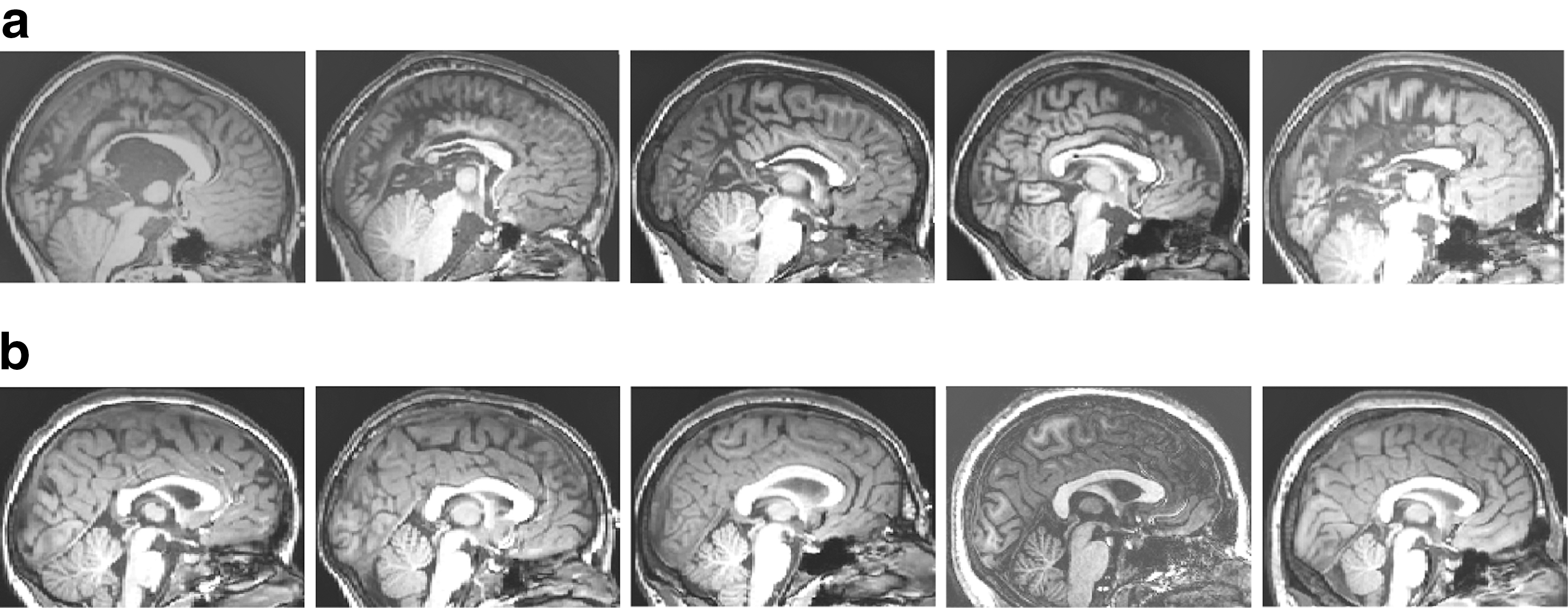
Mid-sagittal MRI cross-sections.
Evaluated using the Edinburgh handedness Inventory Oldfield (1971). Scores below −40=left handed, between −40 and +40=ambidextrous, and above +40=right handed.
Participants with SBH received the four-subtest form of the Stanford–Binet Intelligence test, fourth edition Thorndike et al. (1986), from which a composite was generated.
IQ, intelligence quotient; SBH, spina bifida and hydrocephalus.
MEG recordings
All MEG recordings were conducted using a whole-head neuromagnetometer containing an array of 248 first-order axial gradiometer sensors (WH 3600, 4D Neuroimaging, San Diego, California) housed in a sound-damped and magnetically shielded room. Participants were asked to keep their eyes closed and to avoid blinking or otherwise moving during the recordings. Continuous MEG resting data was collected for each participant (sampling rate of 1017.25 Hz, and 0.1–200 Hz analog band-pass filter). The head position was monitored before and after the data acquisition by using a set of five head position indicator coils. Five minutes of data were available for all controls and three of the SBH children, while 3 min of data were available for the other two. The data were visually inspected for artifacts and noise. Bad channels and time intervals containing noise or artifacts were omitted from the subsequent analysis. This resulted in the removal of two channels for one subject, one channel for eight subjects, and no channels for one subject. The total length of clean time intervals used in the analysis of the control subjects were 138, 171, 243, 252, and 297 sec, while those for the SBH subjects were 117, 159, 237, 252, and 288 sec. The data were zero-phase lowpass filtered and downsampled to a sampling rate of 40.69 Hz, as we chose to study connectivity below 20 Hz. The downsampled data were zero-phase highpass filtered with a 1.5 Hz cutoff Butterworth filter and then segmented into 3-sec segments or epochs. The bootstrap with replacement (Efron and Tibshirani, 1993) was employed to assess the sensitivity of the estimated connectivity to noise. Fifty analyses, that is, MVAR models, were run for each subject using a randomized selection of a subset of epochs out of all the subject's available epochs. The distribution of the estimated cGC depends on the number of epochs used to fit the MVAR model, and the length of available clean data varies for each subject. Hence, we paired subjects in the control and SBH groups when choosing the numbers of epochs to be analyzed in order to ensure that the distributions of the estimates at the group level would be similar under the hypothesis that there is no difference between the groups. Specifically, 39 epochs (117 sec) were used for the control and SBH subjects with the least available data, 53 epochs (159 sec) for the control and SBH subjects with the second smallest available data, and 75 epochs (225 sec) for the remaining three control and SBH subjects.
Methods
The differential pattern of anomalies between posterior and anterior sections of the corpus callosum motivates a comparison of the posterior and anterior interhemispheric effective connectivity. We chose to analyze connectivity between two anterior and two posterior regions of the cortex. The rostral middle frontal regions were selected in part because the middle frontal gyrus and sulcus have the highest percentage of homotopic connections passing through the corpus callosum of any region in the frontal lobes (Jarbo et al., 2012). Inferior and superior parietal lobules were combined for the posterior region because of their integrative role and the types of cognitive deficits in children with SBH. In addition, the superior parietal lobule has one of the highest levels of homotopic connections through the corpus callosum of all regions in the parietal and occipital lobes (Jarbo et al., 2012). The spatial extent of these four regions ensures that the estimated connectivity represents a significant section of the corpus callosum, and, thus, the results should be relatively insensitive to fine structure differences in callosal organization. FreeSurfer (Desikan et al., 2006) was used to automatically identify these cortical regions on each subject's MRI. Figure 2 depicts the four regions analyzed on the cortical surface of one of the control subjects. Figure 3 illustrates the connections involved in the MVAR model for these regions and the connections analyzed in this article.
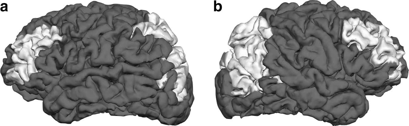
Regions studied in the connectivity analysis shown for one of the control subjects.
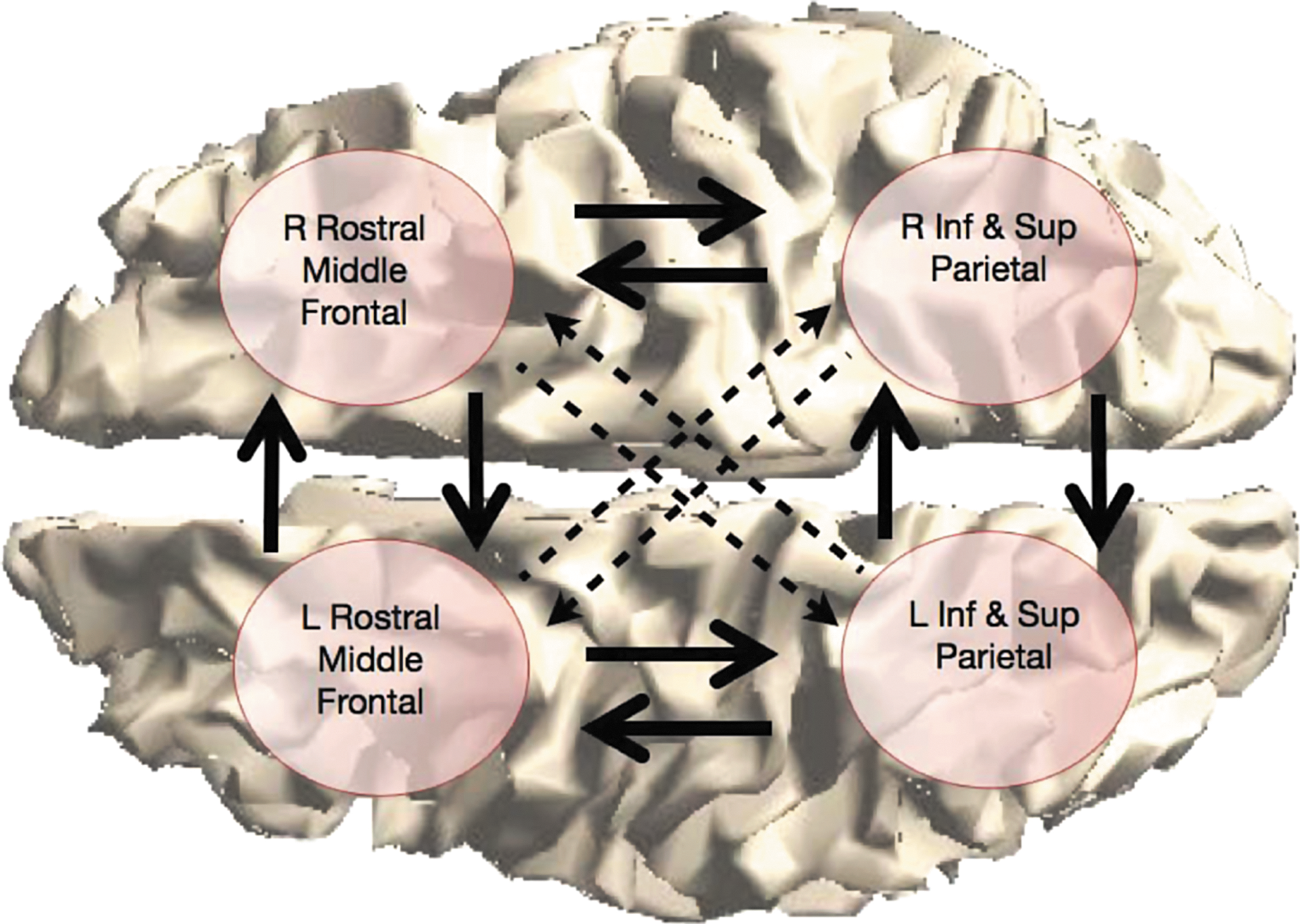
Four-region network representation. The arrows denote the connections included in the multivariable autoregressive model for each subject. The inter- and intra-hemispheric connections depicted by solid arrows are analyzed in this study. Color images available online at
The physics of MEG measurement of cortical activity is represented by computing lead field matrices for all dipoles in each region using a boundary element model (Mosher et al., 1999) obtained from the MNE software (available at:
An MVAR model describes the interactions between the cortical signals as a linear dynamic system, and, thus, is the simplest causal model capable of describing frequency-dependent interactions. Let xm
n,j
be the cortical signal in the mth region at time n and epoch j, define
Here,
The MVAR model parameters
Here,
The cGC as defined by Geweke (1984) is determined from each estimated MVAR model as a measure of effective connectivity. Given three time series gn
, sn
, and zn
, the cGC from z to g is the ratio of the error variance when predicting g using its own past (gn
−
) and the past of s (sn
−
) to that using its own past and the past of s and z (zn
−
); that is, defining
Clearly, the past of z cannot worsen the prediction of gn
and, thus,
The magnitude-squared coherence (MSC) between cortical signals is also calculated from each estimated MVAR model as a measure of functional connectivity. The MSC,
where
then,
contains the auto- and cross-spectral densities for all the cortical signals
We report cGC, MSC, and power on standard frequency bands by integrating the respective measures over the frequency ranges δ (1.5–4 Hz), θ (4–8 Hz), α (8–12 Hz), and β (12–20 Hz).
Results
Figure 4 depicts sample interhemispheric cGC spectra (Equation 3) over 50 random selections of epochs for representative control (top panels) and SBH (bottom panels) subjects. The left panels are the cGC spectra from anterior left to anterior right, and the right panels are the cGC spectra from anterior right to anterior left. Figures 5 and 6 depict the mean interhemispheric cGC and the standard error over 50 random selections of epochs on a subject-by-subject basis. The results for the five control subjects are shown as dark bars on the left of each group, and those for the five SBH subjects are shown as white bars on the right. The order of the bars corresponds to the order of the MRI cross-sections in Figure 1, that is, the left-most control subject bar in Figures 5 and 6 corresponds to the left-most MRI in Figure 1b. Furthermore, the left-most bars in each group denote the subjects with 39 epochs, second from the left denote the subjects with 53 epochs, and the right-most three bars denote the subjects with 75 epochs. This convention also applies to Figures 7, 8, 10 and 11. Figure 5 presents results for the δ and θ bands, while Figure 6 presents results for the α and β bands. In Figures 5 and 6, the top left panel is the cGC from anterior left to anterior right, the top right panel is the cGC from anterior right to anterior left, the bottom left panel is the cGC from posterior left to posterior right, and the bottom right panel is the cGC from posterior right to posterior left. Here, “anterior” refers to the rostral middle frontal regions, while “posterior” refers to the parietal regions.
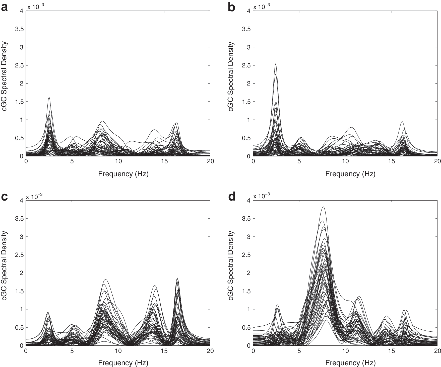
Conditional Granger causality (cGC) spectral density over 50 sets of randomly selected epochs for representative control and SBH subjects.
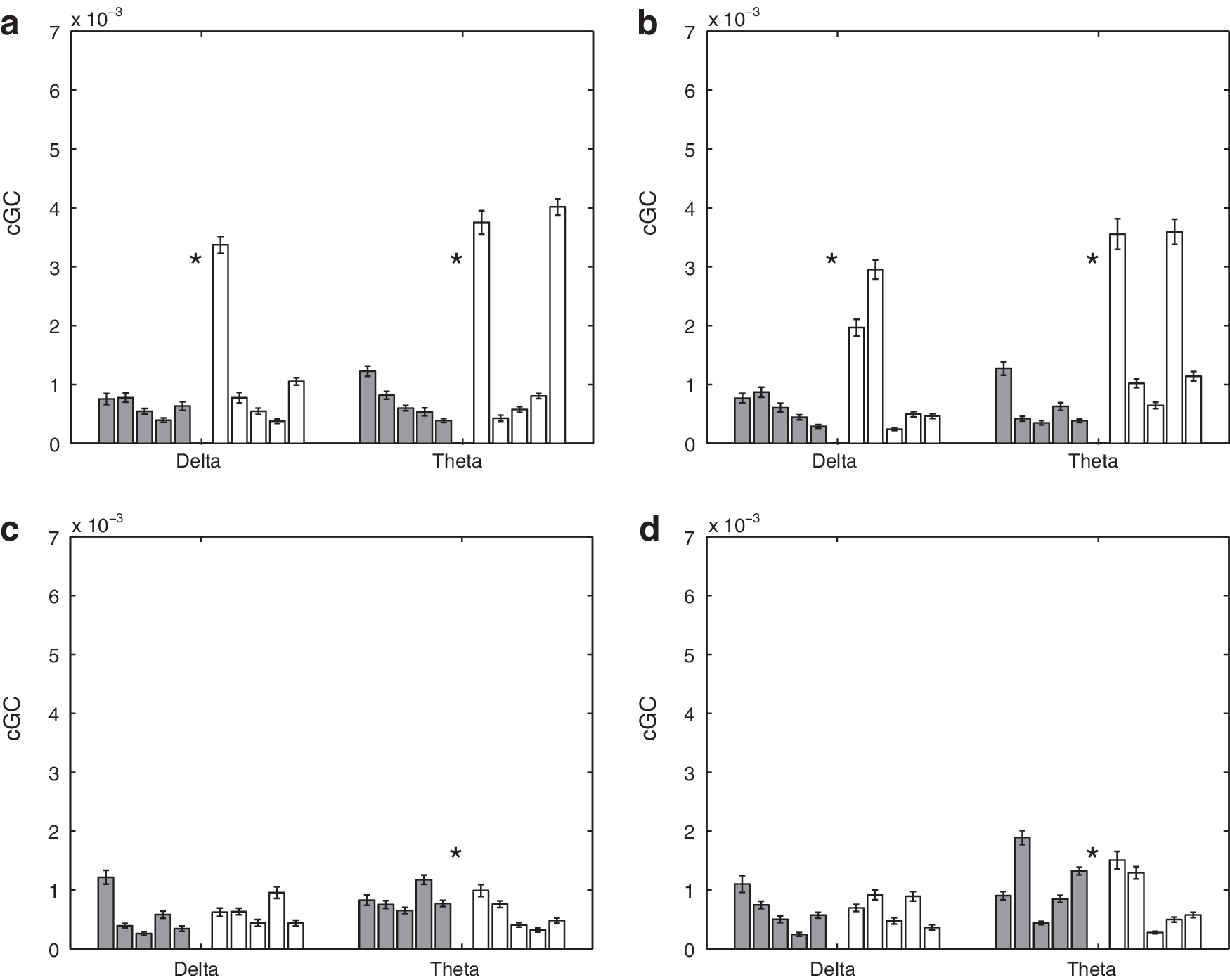
Mean interhemispheric cGC in δ and θ bands over 50 sets of randomly selected epochs for 5 control and 5 SBH subjects. Error bars denote the standard error of the mean. Left (dark) bars represent the control (CN) subjects, and right (white) bars represent the SBH subjects. Asterisks denote bands where the difference between CN and SBH groups are significant at a p<0.01 level after correction for multiple comparisons using false discovery rate (FDR).
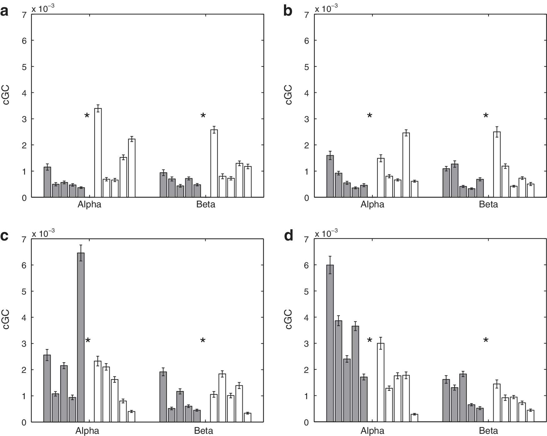
Mean interhemispheric cGC in α and β bands over 50 sets of randomly selected epochs for 5 control and 5 SBH subjects. Error bars denote the standard error of the mean. Left (dark) bars represent the control (CN) subjects, and right (white) bars represent the SBH subjects. Asterisks denote bands where the difference between CN and SBH groups is significant at a p<0.01 level after correction for multiple comparisons using FDR.
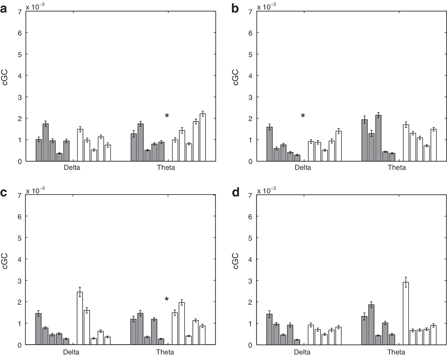
Mean intrahemispheric cGC in δ and θ bands over 50 sets of randomly selected epochs for 5 control and 5 SBH subjects. Error bars denote the standard error of the mean. Left (dark) bars represent the control (CN) subjects, and right (white) bars represent the SBH subjects. Asterisks denote bands where the difference between CN and SBH groups is significant at a p<0.01 level after correction for multiple comparisons using FDR.
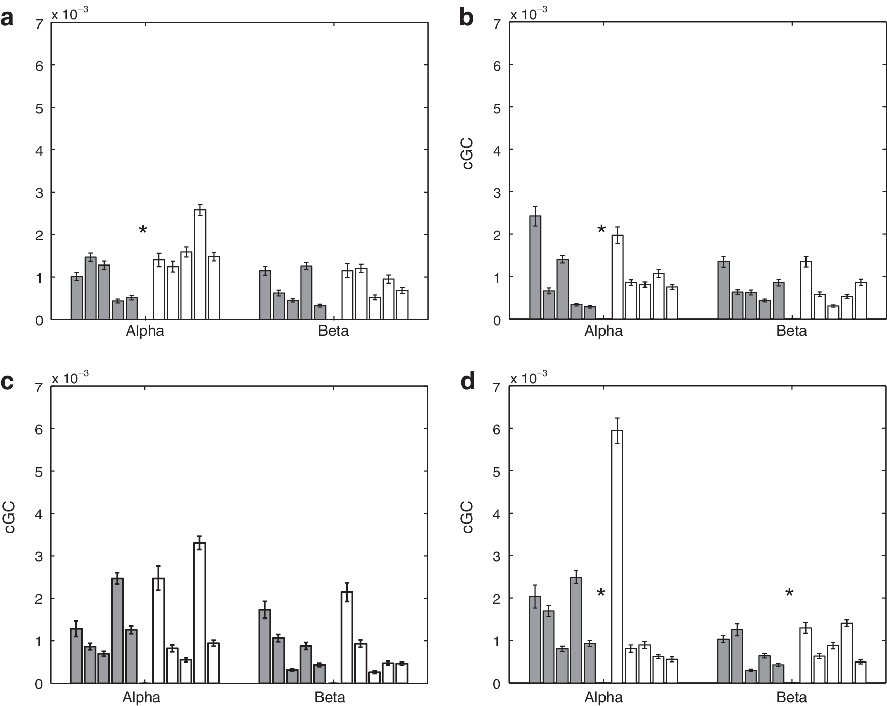
Mean intrahemispheric cGC in α and β bands over 50 sets of randomly selected epochs for 5 control and 5 SBH subjects. Error bars denote the standard error of the mean. Left (dark) bars represent the control (CN) subjects, and right (white) bars represent the SBH subjects. Asterisks denote bands where the difference between CN and SBH groups is significant at a p<0.01 level after correction for multiple comparisons using FDR.
A two-sided nonparametric rank-sum test (Mann–Whitney–U, also called Mann–Whitney–Wilcoxon) is used to test the hypothesis that the cGC values from the control and SBH groups have a shift in distribution. The threshold for declaring a difference is chosen based on a p<0.01 after correction for multiple comparisons using the false discovery rate (FDR) method (Benjamini and Hochberg, 1995). Table 2 presents the test results in the form of p-values for each frequency band and connection depicted in Figures 5 and 6. The differences between 14 of the 16 possible cases are significant as shown by the shaded entries in Table 2.
Shading denotes significant differences between groups at p<0.01 after correction for multiple comparisons using false discovery rate (FDR).
Figures 7 and 8 depict the mean intrahemispheric cGC and standard error over 50 random selections of epochs on a subject-by-subject basis. Figure 7 presents results for the δ and θ bands, while Figure 8 presents results for the α and β bands. In Figure. 7 and 8, the top left panel is the cGC from anterior left to posterior left, the top right panel is the cGC from anterior right to posterior right, the bottom left panel is the cGC from posterior left to anterior left, and the bottom right panel is the cGC from posterior right to anterior right. Table 3 presents the p-values for tests of the intra-hemispheric cGC between the SBH and control groups. Seven of the 16 cases are declared different by the rank-sum test. A visual comparison of Figures 5 –8 suggests that the differences in interhemispheric cGC are generally greater than those in intrahemispheric cGC.
Shading denotes significant differences between groups at p<0.01 after correction for multiple comparisons using FDR.
The average interhemisperic cGC (right-to-left/2+left-to-right/2) over all frequency bands is displayed using a posterior versus anterior format in Figure 9a. The 10 subjects are clustered in two groups, with the SBH subjects generally having an increased anterior cGC and a decreased posterior cGC. Figure 9b depicts the average intrahemispheric cGC (anterior-to-posterior/2+posterior-to-anterior/2) over all the frequency bands in a left hemisphere versus right hemisphere format. The groups do not appear to cluster, although three of the SBH subjects have a slightly higher average left hemisphere cGC than all the control subjects. Table 4 presents the p-values for tests of average wideband inter- and intra-hemispheric cGC between the SBH and control groups. The differences in average wideband interhemispheric cGC are significant for both anterior and posterior connections, while differences in the intrahemispheric average wideband cGC are only found in the left hemisphere.
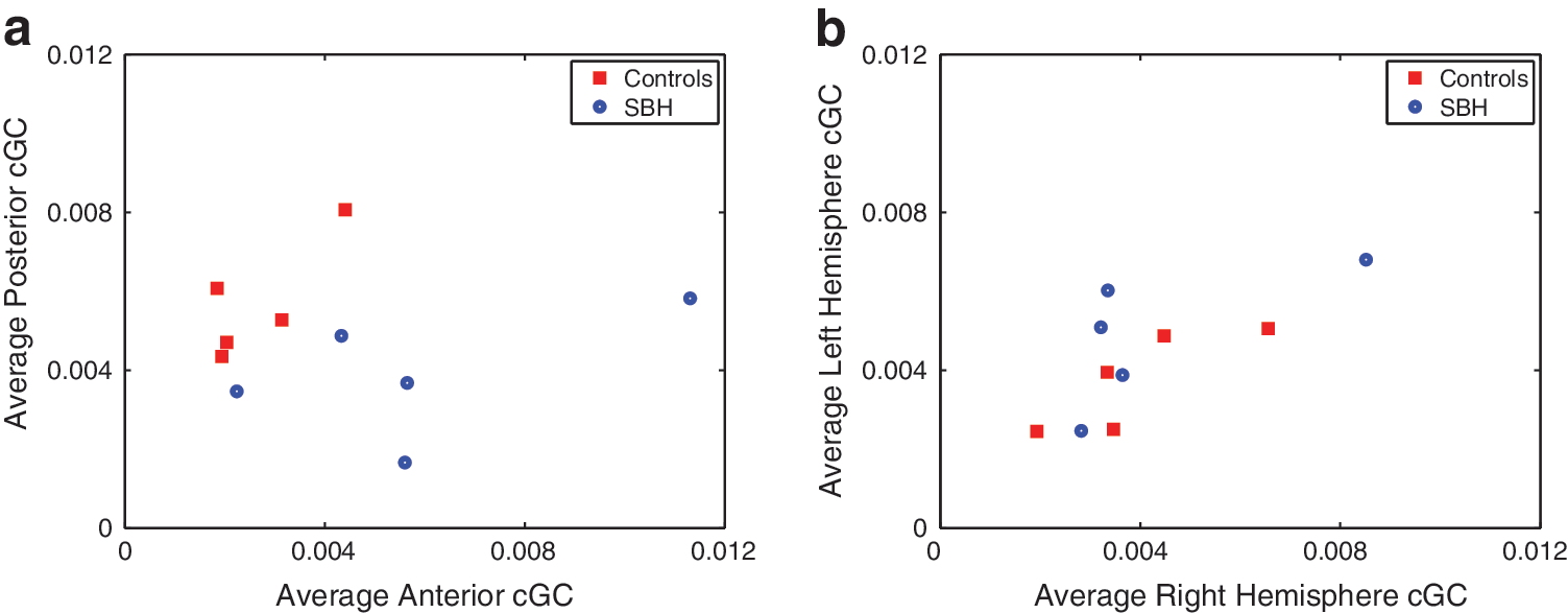
Average of wideband (1.5–20 Hz) cGC for control (CN) and SBH subjects based on 50 sets of randomly selected epochs.
Shading denotes significant differences between groups at p<0.01 after correction for multiple comparisons using FDR.
The average coherence as a function of the frequency band in the front and back is shown in Figure 10. The anterior coherence in the SBH group is generally elevated, while the posterior coherence is reduced relative to the controls. The p-values for tests of coherence between the SBH and control groups are given in Table 5. Five of the eight cases are different at the p<0.01 level, after correction for multiple comparisons using FDR. Figure 11 depicts the power in the back, front, left, and right signals as a function of frequency band for both groups of subjects. The corresponding hypothesis test p-values are provided in Table 6. Seven of the 16 comparisons show significant differences with 6 of those associated with posterior region powers.
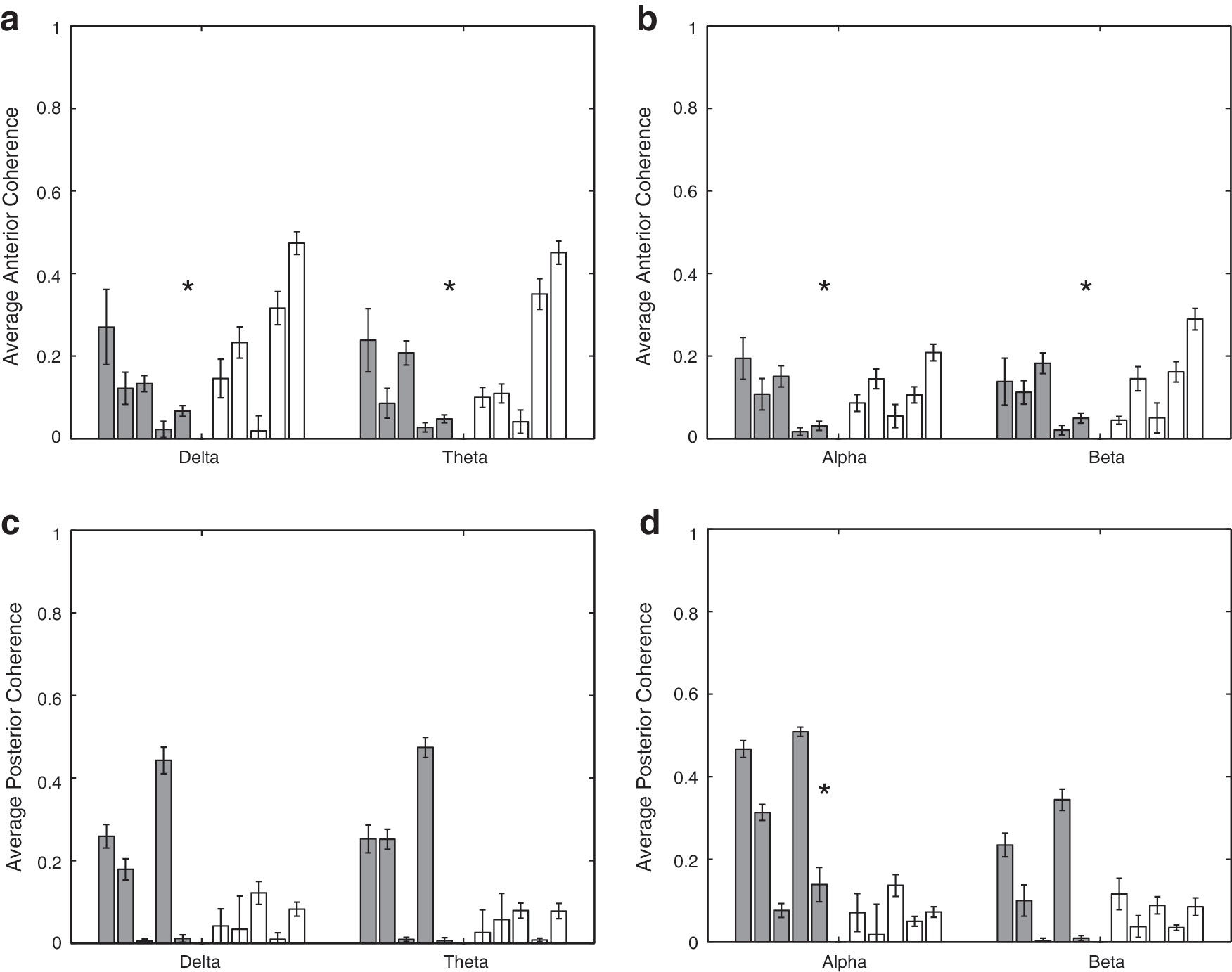
Mean average coherence for each subject over 50 sets of randomly selected epochs. Error bars denote the standard error of the mean. Left (dark) bars represent the control (CN) subjects, and right (white) bars represent the SBH subjects. Asterisks denote bands where the difference between CN and SBH groups is significant at a p<0.01 level after correction for multiple comparisons using FDR.
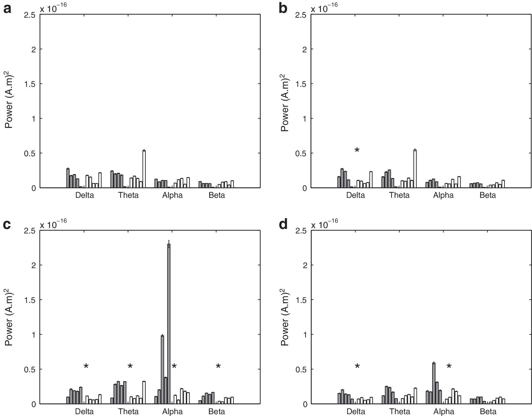
Mean cortical power for each subject over 50 sets of randomly selected epochs. Error bars denote the standard error of the mean. Left (dark) bars represent the control (CN) subjects, and right (white) bars represent the SBH subjects. Asterisks denote bands where the difference between CN and SBH groups is significant at a p<0.01 level after correction for multiple comparisons using FDR.
Shading denotes significant differences between groups at p<0.01 after correction for multiple comparisons using FDR.
Shading denotes significant differences between groups at p<0.01 after correction for multiple comparisons using FDR.
Discussion
We have evaluated the effective (via cGC) and functional (via coherence) inter-hemispheric connectivity between the posterior and anterior homologous cortical areas in a population of SBH and control subjects. This is the first evaluation of cortical effective and functional connectivity in a population with callosal anomolies. The evaluation of interhemispheric connectivity in anterior and posterior regions is motivated by the differential anterior/posterior patterns of anomalies evident in the SBH group.
The SBH subjects generally exhibit significant posterior callosal dysgenesis and/or hypoplasia as shown in Figure 1, and we have found that the posterior power, interhemispheric cGC, and coherence are significantly lower in this group. Reduced effective and functional connectivity are consistent with the cognitive deficits observed in SBH children for operations dependent on the interhemispheric integration of function (Hannay et al., 2008; Klaas et al., 1999). The anterior cGC and coherence are generally higher in the SBH group than the control group. This increase may reflect compensatory mechanisms. The differences in intrahemispheric cGC are generally smaller than those in interhemispheric cGC (Figs. 5 –9, Tables 2 –4). This suggests that the interhemispheric connectivity differences are likely due to callosal anomalies and not a general impairment associated with SBH.
The most striking differences in interhemispheric cGC are found in the θ and α bands as shown in Figures 5 and 6. Elevated anterior cGC is found in the SBH group for both directions in all the frequency bands. The integration of cGC over direction (left to right and right to left) and frequency bands tends to smooth out fluctuations in the data and results in very significant differences between the groups (Table 4). In contrast, the differences in intrahemispheric cGC are less widespread (Figs. 7 and 8). For example, four of the right hemisphere connections/bands are declared different in Table 3, but the differences between the groups are not consistent across connections and frequency bands—averaging over direction and frequency eliminates the distinction between them, as shown in Table 4 and Figure 9.
The anterior coherence in the SBH group is generally higher than that for the controls (Fig. 10, Table 5). The α-band coherence is the only posterior band declared different by the rank-sum test, but this is likely, because two of the control subjects have extremely small δ-, θ-, and β-band posterior coherence. In general, the posterior δ-, θ-, and β-band coherence of the other three control subjects is significantly greater than that of the SBH subjects (Fig. 10). The differences in power between the groups are most significant in the posterior, and, in particular, in the α band, (Fig. 11, Table 6), which is consistent with the scalp level findings reported in Castillo et al. (2009). As a whole, the results suggest that the dominant effect of posterior callosal anomalies in the SBH group is to decrease the posterior effective and functional connectivity and cortical power. A secondary effect appears to be an increase in anterior effective and functional connectivity.
Coherence and cGC are fundamentally different measures of interaction and, thus, are not necessarily proportional to each other, even though they are obtained from an identical MVAR model. Coherence includes the effect of the present values of the signals in each region, while cGC only considers the influence of the past. For example, if two signals are the identical white noise sequence, their MSC is one, while their cGC is zero, because the past does not predict the present. However, both MSC and cGC reveal the effects of callosal anomalies on connectivity at the group level. Similarly, cortical power is not directly related to functional or effective connectivity. Although the relationships between power, coherence, and cGC vary in individual subjects, power also reveals a consistent difference at the group level. Our results suggest that effective and functional connectivity are more sensitive indicators of the differences between groups than power. In particular, both cGC and coherence indicate anterior differences that are not evident in cortical power.
Cortical cGC and coherence values vary across the individuals in each group. The variability across the 50 analyses for each subject are consistently small relative to the variations between subjects, which suggests that the individual differences are not due to estimation (noise driven) effects. The differences likely reflect the differences in cortical organization with regard to the cortical regions analyzed.
The rank-sum test used to compare control and SBH subjects does not impose any distributional assumptions on the data. It is relatively insensitive to absolute amplitudes, as it ranks the observations and evaluates the probability that the observed ordering is due to identical probability distributions for the groups. There are two sources of variability that are addressed by the test: within subject estimation variability, that is, the fact that repeated estimates of a fixed underlying connectivity will vary due to noise and other random effects, and variability between the subjects in a group. The bootstrap procedure explicitly account for within subject estimation variability. It is possible, although extremely unlikely, that the five subjects in each group are not representative of their populations.
The magnitudes of the cGC values are generally small. Since cGC is the logarithm of the ratio of prediction error variances and log(1+x)≈x for x small, a cGC of 0.01 implies that the past of the candidate region cortical signal reduces the prediction error variance of the test region signal by ∼1%. There are several possible reasons for the small cGC values that are observed. First, the effective connectivity between hemispheres may be small in the absence of a task requiring interhemispheric interaction, which is consistent with neuropsychological studies (Hannay et al., 2008). The rhythmic oscillations that tend to dominate the eyes-closed resting condition are very well explained by their own past. Second, it is likely that there are a large number of independent influences affecting the signals in each region, and, thus, the other regions only predict a small fraction of the activity. It is also possible that the effective connectivity is not stationary over the analysis interval. If, for example, the states of relatively low connectivity alternate with the states of higher connectivity as postulated by the microstate theory (e.g., Lehmann et al., 1998), then the average cGC over an interval of several minutes may be small. A similar spatial averaging effect may be present. We are representing fairly large cortical regions with a single time series. If there are local areas within each region that have high effective connectivity and others that are not interacting, then the average cGC over the region may be small. Finally, the MVAR model only captures linear relationships. Any nonlinear interactions are not represented. In spite of the small magnitude of the cGC, it is consistent across the 10 analyses for each subject, and it reveals consistent differences that concur with coherence and the callosal anomalies of the SBH group.
Representation of the activity of a cortical region with a single signal is common in connectivity analysis. For example, Babiloni et al. (2005) used a linear minimum norm inverse problem solution to estimate the cortical currents for a distributed source model of about 5000 dipoles. Next, they collapsed these 5000 time series into a single net time series for each region of interest by averaging the magnitudes of all dipole currents within the region. Clearly, it is not possible to capture the full complexity of the cortical current distribution over a region with a single signal, so such representations may be interpreted as equivalent sources, analogous to the widely used equivalent current dipole (e.g., Baillet et al., 2001). In the approach used here, the basis coefficients adapt the spatial pattern of this equivalent source representation to the individual activity distribution in the region. Here, we used three bases with relatively large cortical regions. This results in a model that captures the average behavior across the region, an intentional choice to reduce the sensitivity of the analysis to individual differences in cortical organization and callosal anomalies. It also limits the sensitivity of the analyses to the automated region extraction process. The results indicate that this modeling approach is effective at capturing connectivity differences between the control and SBH groups.
Our estimation of effective connectivity involves a generative model relating the signals in different regions and is subject to errors of omission. For example, unmodeled common sources can distort connectivity conclusions. Modeling the entire brain at high resolution is currently intractable. However, an important attribute of a model is its predictive ability. The model used here correctly differentiates the controls and SBH groups. A common modeling problem, particularly important when using EEG or MEG data due to low signal-to-noise ratio and the ill-posed nature of the inverse problem, is the reliable estimation of model parameters. The consistency of the differences between groups and the small variability over different random selections of epochs for each subject suggest that the algorithm employed here (Cheung et al., 2010) provides reliable estimates.
Conclusions
Posterior effective and functional connectivity between hemispheres is generally reduced in children with spina bifida. This observation is consistent with the callosal anomalies and cognitive deficits typical to this population. Posterior cortical power is also reduced. Anterior effective and functional interhemispheric connectivity is generally increased in spina bifida, a result that may reflect compensatory mechanisms. The differences between spina bifida and control groups are generally most significant in the θ and α bands. In contrast, intrahemispheric effective connectivity is generally similar in the control and spina bifida groups.
Footnotes
Acknowledgments
This research was supported in part by grants R21EB009749 awarded to BVV from the National Institute of Biomedical Imaging and Bioengineering and P01-HD35946 awarded to JMF from the National Institute of Child Health and Human Development (NICHD). The content is solely the responsibility of the authors and does not necessarily represent the official views of the NIBIB, NICHD, or the National Institutes of Health. The authors thank Dr. Scott Rand from the Medical College of Wisconsin for help with ![]() and the anonymous reviewers for suggestions that significantly improved the article. This research was performed using resources and the computing assistance of the UW-Madison Center For High Throughput Computing.
and the anonymous reviewers for suggestions that significantly improved the article. This research was performed using resources and the computing assistance of the UW-Madison Center For High Throughput Computing.
Author Disclosure Statement
None of the authors have potential conflicts of interest with regard to this study.