Fast Eigenvector Centrality Mapping of Voxel-Wise Connectivity in Functional Magnetic Resonance Imaging: Implementation,Validation,and Interpretation

Abstract

Eigenvector centrality mapping (ECM) has recently emerged as a measure to spatially characterize connectivity in functional brain imaging by attributing network properties to voxels. The main obstacle for widespread use of ECM in functional magnetic resonance imaging (fMRI) is the cost of computing and storing the connectivity matrix. This article presents fast ECM (fECM), an efficient algorithm to estimate voxel-wise eigenvector centralities from fMRI time series. Instead of explicitly storing the connectivity matrix, fECM computes matrix–vector products directly from the data, achieving high accelerations for computing voxel-wise centralities in fMRI at standard resolutions for multivariate analyses, and enabling high-resolution analyses performed on standard hardware. We demonstrate the validity of fECM at cluster and voxel levels, using synthetic and in vivo data. Results from synthetic data are compared to the theoretical gold standard, and local centrality changes in fMRI data are measured after experimental intervention. A simple scheme is presented to generate time series with prescribed covariances that represent a connectivity matrix. These time series are used to construct a 4D dataset whose volumes consist of separate regions with known intra- and inter-regional connectivities. The fECM method is tested and validated on these synthetic data. Resting-state fMRI data acquired after real-versus-sham repetitive transcranial magnetic stimulation show fECM connectivity changes in resting-state network regions. A comparison of analyses with and without accounting for motion parameters demonstrates a moderate effect of these parameters on the centrality estimates. Its computational speed and statistical sensitivity make fECM a good candidate for connectivity analyses of multimodality and high-resolution functional neuroimaging data.

Introduction

T he analysis of connectivity between different regions in the brain is one of the oldest topics in neuroscience [see (Graves, 1997) and references therein]. Modern neuroimaging modalities, such as functional magnetic resonance imaging (fMRI), diffusion tensor imaging (DTI), and electroencephalography (EEG), are providing new insights into the strength of connections between regions in vivo (Hagmann et al., 2010; Wendling et al., 2009). Different analysis techniques have been successfully applied to these data, for example, independent component analyses (ICA) of resting-state fMRI (RS-fMRI) data (Beckmann et al., 2005), graphs of connections between regions detected in a task-based fMRI experiment (Bullmore et al., 2000), and intermodality correspondence, for example, histological data and fiber tracts detected by DTI (Zhang et al., 2010).

The recent introduction of centrality analyses (Sporns et al., 2007) to functional neuroimaging combines the high spatial resolution of voxel-based methods, such as ICA, and the interpretability of connectivity matrices used in graph analyses (e.g., Salvador et al., 2005). Centrality is a property of a node that quantifies its prominence in a network. Different centrality measures are (1) degree centrality, counting the node's direct connections, (2) betweenness centrality, computing the proportion of shortest paths going through the node, (3) leverage centrality, computing how much other nodes rely on the observed node for their connections, (4) subgraph centrality, characterizing the node's participation in different subgraphs of the network, and (5) eigenvector centrality, the sum of centralities of the node's direct neighbors (Joyce et al., 2010; Lohmann et al., 2010; Zuo et al., 2012).

A common problem of whole-brain voxel-wise centrality analyses is the size of the intermediate connectivity matrix, which is the square of the number of brain voxels. At a fairly standard resolution of 3 mm isotropic and 40,000 voxels, it takes about 6 GB to store the complete matrix (Lohmann et al., 2010). Computing the connectivity matrix is the most time-consuming operation for most whole-brain voxel-wise centrality analyses; analyses at higher resolutions are not possible on standard hardware without sparsening the voxel-wise matrix, for example, by thresholding and/or binarizing (Van den Heuvel et al., 2008). A commonly used alternative for voxel-wise whole-brain connectivity analyses is to consider inter-regional connections, thereby sacrificing the spatial resolution of fMRI. Regions can be defined by anatomical atlases (Sanz-Arigita et al., 2010) or previous analyses (Bullmore et al., 2000).

We present fast eigenvector centrality mapping (fECM), a method to compute eigenvector centrality maps from voxel-wise connectivities in fMRI data. Instead of explicitly computing and storing the connectivity matrix, the algorithm directly computes its product with the eigenvector estimate at each iteration. The fECM method provides a significant computational gain and a decrease in memory consumption, compared to the explicit matrix computation.

In this article, we review the ECM technique and introduce the fECM algorithm. We describe the construction of synthetic data time series representing interconnected regions, and a 4D synthetic dataset based on these regional time series, where voxel time series inside each region are made from the regional signals. We review the computation times required for analyzing these datasets and describe the analyses of the synthetic 4D data in terms of (1) the synthetic regional time series and (2) their relation to the ground truth eigenvectors.

In an fMRI experiment, RS-fMRI is measured after low-frequency repetitive transcranial magnetic stimulation (1 Hz rTMS) and after a control condition (sham rTMS). We assess the differences between the experimental conditions with fECM in two separate analyses: one without including motion parameters and one that includes the motion parameters as confounds. These fECM results are tested for condition-specific differences using nonparametric cluster statistics.

There is little literature on ECM differences after rTMS interventions. Previous analyses of the same data used regression of blood oxygenation level-dependent fluctuations, followed by parametric testing, to measure resting-state changes after rTMS (Van der Werf et al., 2010). Data from a task-based study using general linear model (GLM) analyses (Van den Heuvel et al., 2011) revealed local and distal changes in activity after rTMS. We discuss our findings and compare them to these earlier results.

With these findings, we demonstrate the validity of the fECM method and the computational advantage of the new algorithm. We compare fECM differences in the RS-fMRI dataset with our hypotheses and previous analyses.

Materials and Methods

Fast eigenvector centrality mapping

ECM attributes importance to a network node based on its connections to other important nodes (Bonacich, 1987). If importance is assigned via the number of connections, then important nodes have many connections to other nodes with many connections. One of the best-known applications of eigenvector centrality is Google's PageRank algorithm (Bryan and Leise, 2006), which assigns high relevance to Web pages if they are linked to many other relevant Web pages. ECM has recently been introduced as a tool for measuring the importance of points in brain networks (Lohmann et al., 2010) and shown to compare favorably to other centrality measures (Joyce et al., 2010). The use of voxel-wise centrality measures in fMRI enables visualization of connectivity on the finest scale available in brain images: every voxel location has its own measure of relevance to the network. Eigenvector centrality can be measured in other modalities for neuroscientific data analysis; we will discuss the methods assuming fMRI time series.

Let Y _nt denote the fMRI signal at time t=1, …, T and voxel n=1, …, N. As N is generally large—in Montreal Neurological Institute (MNI) standard space with 2×2×2 mm³ voxels, N=902,629—removing non-brain voxels from the ECM analysis is not enough to make current methods run on desktop computers: it is also necessary to resample the images at lower resolutions (Joyce et al., 2010; Lohmann et al., 2010; Zuo et al., 2012), potentially degrading the image quality. Using the definition of correlation and the power iteration algorithm, it is possible to improve the efficiency of fECM.

The direct correlation r _nn between voxel n and n′ can be expressed as \documentclass{aastex}\usepackage{amsbsy}\usepackage{amsfonts}\usepackage{amssymb}\usepackage{bm}\usepackage{mathrsfs}\usepackage{pifont}\usepackage{stmaryrd}\usepackage{textcomp}\usepackage{portland, xspace}\usepackage{amsmath, amsxtra}\pagestyle{empty}\DeclareMathSizes{10}{9}{7}{6}\begin{document}\begin{align*}R_ { nn { \prime } } = \frac { \sum_j ( Y_ { nj } - \bar { Y } _ { n } ) ( Y_ { n { \prime } j } - \bar { Y } _ { n { \prime } } ) } { \sqrt { \sum_j ( Y_ { nj } - \bar { Y } _n ) ^2 } \sqrt { \sum_j ( Y_ { n { \prime } j } - \bar { Y } _ { n { \prime } } ) ^2 } } \tag { 1 } \end{align*}\end{document}

where \documentclass{aastex}\usepackage{amsbsy}\usepackage{amsfonts}\usepackage{amssymb}\usepackage{bm}\usepackage{mathrsfs}\usepackage{pifont}\usepackage{stmaryrd}\usepackage{textcomp}\usepackage{portland, xspace}\usepackage{amsmath, amsxtra}\pagestyle{empty}\DeclareMathSizes{10}{9}{7}{6}\begin{document}$$\bar{Y}_n$$\end{document} is the time-series mean at voxel location n. In a matrix form, this can be expressed as \documentclass{aastex}\usepackage{amsbsy}\usepackage{amsfonts}\usepackage{amssymb}\usepackage{bm}\usepackage{mathrsfs}\usepackage{pifont}\usepackage{stmaryrd}\usepackage{textcomp}\usepackage{portland, xspace}\usepackage{amsmath, amsxtra}\pagestyle{empty}\DeclareMathSizes{10}{9}{7}{6}\begin{document}\begin{align*}R = D^{ - \it1} Y P Y^T D^{ - \it1} \tag{2}\end{align*}\end{document}

where D is a diagonal matrix containing the voxel variances, and P is the projection operator removing the time-series mean of every voxel: \documentclass{aastex}\usepackage{amsbsy}\usepackage{amsfonts}\usepackage{amssymb}\usepackage{bm}\usepackage{mathrsfs}\usepackage{pifont}\usepackage{stmaryrd}\usepackage{textcomp}\usepackage{portland, xspace}\usepackage{amsmath, amsxtra}\pagestyle{empty}\DeclareMathSizes{10}{9}{7}{6}\begin{document}\begin{align*} & P = I - \frac {{\bf e}^{\prime} {\bf e}^T} {{\bf e}^T {\bf e}} \\& {\rm with} \ {\bf e} = (1 , 1 , \ldots 1)^T \\& D = diag \left( \frac {1} {\sqrt {\sum_j (YP) _{1 , j} ^2}} , \frac {1} {\sqrt {\sum _j(YP) _ {2 , j} ^2}} , \cdots \frac {1} {\sqrt {\sum_j (YP) _ {N , j} ^2}} , \right) \tag{3} \end{align*}\end{document}

Using the correlation matrix R to represent voxel-wise connectivity, ECM finds the vector v that satisfies \documentclass{aastex}\usepackage{amsbsy}\usepackage{amsfonts}\usepackage{amssymb}\usepackage{bm}\usepackage{mathrsfs}\usepackage{pifont}\usepackage{stmaryrd}\usepackage{textcomp}\usepackage{portland, xspace}\usepackage{amsmath, amsxtra}\pagestyle{empty}\DeclareMathSizes{10}{9}{7}{6}\begin{document}\begin{align*}R { \bf v} = \lambda { \bf v}. \tag{4}\end{align*}\end{document}

In this equation, vector v is an eigenvector of matrix R, and scalar λ is its corresponding eigenvalue. According to the Perron-Frobenius theorem (Bryan and Leise, 2006), the dominant eigenvector of a matrix M is uniquely determined, and its coefficients and eigenvalue are positive and real-valued, if all coefficients of M are positive, or if they are non-negative and M is irreducible.

The power iteration method (Golub and Van der Vorst, 2000) to find the dominant eigenvector, which is the eigenvector with the largest eigenvalue, can be expressed as \documentclass{aastex}\usepackage{amsbsy}\usepackage{amsfonts}\usepackage{amssymb}\usepackage{bm}\usepackage{mathrsfs}\usepackage{pifont}\usepackage{stmaryrd}\usepackage{textcomp}\usepackage{portland, xspace}\usepackage{amsmath, amsxtra}\pagestyle{empty}\DeclareMathSizes{10}{9}{7}{6}\begin{document}\begin{align*}\begin{cases} \tilde { \bf v } ^ { i + 1 } = R { \bf v } ^i \\ \\ { \bf v } ^ { i + 1 } = \displaystyle \frac { \tilde { \bf v } ^ { i + 1 } } { \mid \mid \tilde { \bf v } ^ { i+ 1 } \mid \mid } \end{cases} \tag { 5 } \end{align*}\end{document}

Using this algorithm, only matrix–vector products of the connectivity matrix and a series of vectors are needed, and not the connectivity matrix itself. Therefore, in our implementation, we compute these matrix–vector products as \documentclass{aastex}\usepackage{amsbsy}\usepackage{amsfonts}\usepackage{amssymb}\usepackage{bm}\usepackage{mathrsfs}\usepackage{pifont}\usepackage{stmaryrd}\usepackage{textcomp}\usepackage{portland, xspace}\usepackage{amsmath, amsxtra}\pagestyle{empty}\DeclareMathSizes{10}{9}{7}{6}\begin{document}\begin{align*}R \ { \bf v}^i = ( D^{ - \it1} Y P ) \ ( ( D^{ - \it1} YP ) ^T { \bf v}^i ) , \tag{6}\end{align*}\end{document}

using the property of projection operators that P=P ^T=P ². The matrix D ⁻¹ YP, containing the time series with zero mean and unit variance, only needs to be computed once. Only NT floating-point numbers need to be stored, as opposed to N ² numbers for the complete matrix R. Similarly, the number of multiplications is reduced from N ² to 2NT.

One of the benefits of this formulation is that by using the projection matrix P, it can be generalized to definitions of R where other confounding signals are removed from the data, such as breathing, heartbeat, and mean image intensity variability (De Munck et al., 2008).

Because correlations can be negative as well as positive, we use a distance-related measure to quantify connectivity to obtain a connectivity matrix with only non-negative elements. For two time signals Y_n and Y_n′ with mean zero and unit variance, the following holds for the (L2) distance Δ_nn′: \documentclass{aastex}\usepackage{amsbsy}\usepackage{amsfonts}\usepackage{amssymb}\usepackage{bm}\usepackage{mathrsfs}\usepackage{pifont}\usepackage{stmaryrd}\usepackage{textcomp}\usepackage{portland, xspace}\usepackage{amsmath, amsxtra}\pagestyle{empty}\DeclareMathSizes{10}{9}{7}{6}\begin{document}\begin{align*} \begin{split} \Delta_{nn{ \prime}}^2 & = \mid \mid Y_n - Y_{n{ \prime}} \mid \mid ^2 \\& = \mid \mid Y_n \mid \mid ^2 + \mid \mid Y_{n{ \prime}} \mid \mid ^2 - 2 Y_n Y_{n{ \prime}} \quad 0 \leq \Delta_{nn{ \prime}}^2 \leq 4 \\& = 2 - 2r_{nn{ \prime}},\end{split} \tag{7}\end{align*}\end{document}

and we can define a connectivity measure that decreases with increasing distance, as \documentclass{aastex}\usepackage{amsbsy}\usepackage{amsfonts}\usepackage{amssymb}\usepackage{bm}\usepackage{mathrsfs}\usepackage{pifont}\usepackage{stmaryrd}\usepackage{textcomp}\usepackage{portland, xspace}\usepackage{amsmath, amsxtra}\pagestyle{empty}\DeclareMathSizes{10}{9}{7}{6}\begin{document}\begin{align*}c_ { nn { \prime } } = 1 - \frac { \Delta_ { nn { \prime } } ^2 } { 4 } = \frac { 1 + r_ { nn { \prime } } } { 2 } \tag { 8 } \end{align*}\end{document}

The matrix C satisfies the conditions of the Perron-Frobenius theorem, which guarantees that the dominant eigenvector has positive coefficients. Using this definition for connectivity, the iterations in Equation (5) are implemented as \documentclass{aastex}\usepackage{amsbsy}\usepackage{amsfonts}\usepackage{amssymb}\usepackage{bm}\usepackage{mathrsfs}\usepackage{pifont}\usepackage{stmaryrd}\usepackage{textcomp}\usepackage{portland, xspace}\usepackage{amsmath, amsxtra}\pagestyle{empty}\DeclareMathSizes{10}{9}{7}{6}\begin{document}\begin{align*} C {\bf v}^i &= \frac{{\bf e} {{\bf e}^T} {{\bf v}^i} + R {{\bf v}^i}}{2} \\ & = \frac {{\bf e}}{2} \left( {\bf e}^T {{\bf v}^i}\right) + \frac {1} {2} \left((D^{ - 1}YP) (D^{- 1}YP)^T{{\bf v}^i} \right) \tag{9}\end{align*}\end{document}

The power iteration algorithm using Equation (9) [a modified version of Eq. (6)] does not require the storage of C or R. Starting with a constant vector v ⁰, the algorithm repeats Equation (9) until a convergence criterion is used—in this article, we use a difference ∥v ⁱ −v ⁱ⁺¹∥ of <0.1% of ∥v ⁱ∥. In this study, we found that the algorithm always converged after around 10 iterations.

Equation (8) shows that this connectivity measure is almost identical to the correlation, increased by 1 to avoid negative numbers, as used previously (Lohmann et al., 2010). However, it is misleading to regard these values, which are squared distances between normalized vectors, as correlation values. While the transformation from R to C is trivial (adding a constant to all elements), the eigenvectors of C do not follow trivially from the eigenvectors of R.

The final vector v is multiplied by a factor √2 to ensure node centrality (Joyce et al., 2010; Ruhnau, 2000), which means that (1) all centrality values are between 0 and 1, and (2) only center nodes in star networks, independent of network size, have value 1. A star network of N nodes has exactly N-1 connections, from the center to the N-1 leaves.

Synthetic data

In the current fMRI literature, there is no mention of testing centrality measures on synthetic data. We constructed synthetic time series data representing temporally correlated processes, to test whether

1. a precisely specified connectivity pattern can be represented by correlated time series;

2. the vector returned by fECM approximates the dominant eigenvector of that pattern;

3. the specified connectivity between clusters is also represented in the voxels of those clusters.

A test dataset was generated as follows:

First, an adjacency matrix A for a network of 27 nodes was constructed using an undirected Barabási-Albert randomnetwork model (Barabási and Albert, 1999), implemented in the igraph (http://igraph.sourceforge.net) package in the R (www.r-project.org) statistical computing environment.

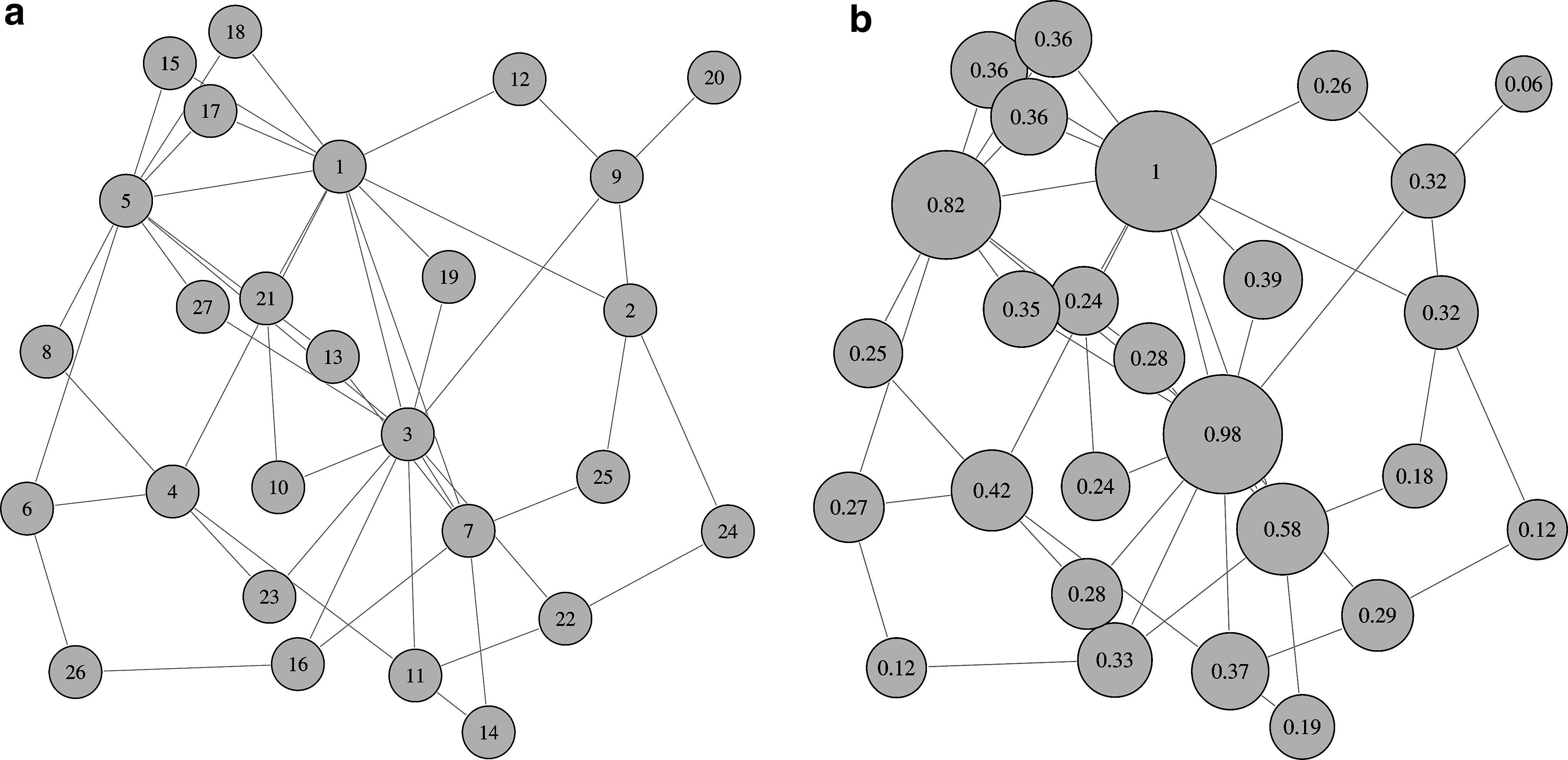
An optimal layout was produced in the visualization program Tulip (http://tulip.labri.fr) by starting with a circular layout and then applying the force-directed Fruchterman-Reingold layout algorithm. This graph is shown in Figure 1a. In Figure 1b, each node's size represents its eigenvector centrality, which is also written in the node.

FIG. 1.

Layout of the simulated network: (a) labels shown inside the nodes and (b) eigenvector centrality shown as node sizes and printed in the nodes.

Using this graph, representative time series X_nt were generated for every node as follows:

1. let the binary (symmetric) adjacency matrix A represent connections between the 27 nodes;

2. let the positive definite matrix A′=I₂₇ +θ A, with I₂₇ the identity matrix (see Fig. 2a);

3. let X′ ∼ N(0,1) be a 200×27 matrix and X=X′ chol(A′)

Here, θ was the reciprocal of the largest absolute eigenvalue of A, and chol (A′) the Cholesky decomposition of A′ yielding its matrix root. The resulting matrix X contained 27 time series of length 200 with Gaussian distributed values whose sample covariance matrix (see Fig. 2b) closely resembled A.

FIG. 2.

(a) A positive definite matrix A′, created by adding the identity matrix to a weighted version of an adjacency matrix A. (b) Covariance matrix of 27 activity time-series X. (c) Labels of the 27 regions in a volume of the masked 4D test dataset.

A 4D time series of image volumes was created from a template of a T2-weighted image in the MNI standard space (Mazziotta et al., 2001), by clipping away non-brain voxels and downsampling it using third-degree B-spline resampling (Thevenaz et al., 2000). The resulting image of 27×36×18 voxels was copied 200 times to form the baseline time series. For each of the 27 regions of 9×12×6 voxels (see Fig. 2c), the corresponding column from the matrix X was added to the baseline signal, so that

1. every voxel inside a region had the same underlying activity signal;

2. the activity signals of the 27 regions had known connectivities.

Finally, Gaussian noise was added to all voxels' time signals. Thus, every voxel location in the resulting 4D dataset D contained a noisy version of the regional signal similar to the time signals of other voxels in the same cluster, whose base signal in turn had a known connectivity to the other clusters.

The fECM values computed from X were compared with the theoretical values given by MatLab (The MathWorks, Natick, MA) routines. Voxel-wise ECM values were computed by an in-house C++ program, which takes a 4D nifti file (http://nifti.nimh.nih.gov) as its input and produces a 3D nifti file containing an eigenvector centrality map.

In brain connectivity analyses, the connectome is a mix of local, within-cluster connections, and global between-cluster connections (Achard et al., 2006). To study the effect of cluster size on voxel-wise centralities, we performed two fECM analyses: one without masking, using all voxel locations to guarantee equal cluster sizes, and one after masking the volumes with a brain shape, resulting in unequal cluster sizes.

Real data

Subjects were recruited from university students and staff, and had given their informed consent before the experiment. All procedures complied with the guidelines described in the Declaration of Helsinki and were approved by the Medical Ethics Board of the VU University Medical Center.

RS-fMRI data were acquired twice in 10 healthy right-handed controls (six women, mean age 25.5 years) as described before (Van der Werf et al., 2010): immediately after 20 min of either low-frequency (1 Hz) repetitive rTMS or sham stimulation of equal duration, on two separate days in balanced order. The coil, a hand-held figure-of-eight coil (MedTronic MagOption) was placed on the left dorsolateral prefrontal cortex, 5 cm anterior to the location where stimulation yielded the strongest motor responses in the contralateral hand. The intensity of stimulation was chosen so that a minimum of five visible hand/finger responses were observed in a series of 10 stimulations on the hand area of the primary motor cortex.

Scanning was done immediately after the rTMS experiment, using a 3T Intera MR scanner (Philips Medical Systems, Best, The Netherlands) and the following parameters for the echo planar imaging sequence: repetition time 2.3 sec, echo time 30 msec, and 160 volumes containing 96×96×35 voxels of 2.3×2.3×3.0 mm³. During the acquisition, subjects were instructed to lie still in the scanner with their eyes closed without falling asleep. A high-resolution anatomical 3D image was acquired during the same scan session, using the following settings: gradient echo T1-weighted sequence, 170 sagittal slices of 256×256 voxels, and voxel size 1×1×1 mm³.

The images were preprocessed in FSL (Smith et al., 2004) which included removal of non-brain tissue, motion correction, high-pass temporal filtering (cutoff 100 sec), smoothing with a Gaussian kernel (full width at half maximum [FWHM] 6 mm isotropic), and rigid-body coregistration to the T1-weighted image, matching the previous analysis of these data (Van der Werf et al., 2010). After affine mapping into MNI standard space (Mazziotta et al., 2001), data were resampled at a resolution of 2×2×2 mm³ (instead of 4×4×4 mm³ as previously), which is the default in most fMRI analyses, and the resolution of all fMRI templates and atlases.

The smoothing kernel was chosen to match previous analyses of these data (Van der Werf et al., 2010). Because smoothing introduces local spatial dependencies that may bias centrality estimates (Zuo et al., 2012), fECM was also estimated after preprocessing with minimal (FWHM 3 mm) and without smoothing. However, the power iteration algorithm failed to converge on most of the datasets when no smoothing was used. Convergence improved after minimal smoothing, but was still problematic for more than half of the datasets. With the original smoothing parameters (Van der Werf et al., 2010), the algorithm converged quickly without the need to resample at a lower spatial resolution (which would also artificially group together functionally unrelated voxels). Another effect of smoothing is that it precludes local deviations introduced by resampling in standard space, improving robustness (Sepulcre et al., 2010).

Before analysis, all standard-space time-series were masked to only contain brain voxel locations included in every subject, by multiplying an MNI-space brain mask by the intersection of all subject-specific masks, followed by a mask that excluded all regions containing cerebrospinal fluid.

The resulting time series were analyzed by the fECM program, yielding a 3D voxel-wise map per subject. Recent studies have measured significant influences of head motion parameters on functional brain connectivity estimates (Power et al., 2012; Satterthwaite et al., 2012; Van Dijk et al., 2012). To measure the effect of head motion parameters on the estimated centralities, each single-session analysis was done twice: once in its simplest form, and once with the volume-wise motion parameters included in P [see Eqs. (6) and (9)] to remove effects of head motion from the time signals.

After Gaussian smoothing (FWHM 5 mm isotropic) of subject-specific fECMs, differences between the post-rTMS and post-sham were assessed in group-level analyses using a paired GLM test to compute group-wise differences, and a cluster-wise permutation-based method (Bullmore et al., 1999) to determine significance. In each analysis, a cluster-forming threshold was automatically determined to maximize the number of suprathreshold clusters in the null distribution. Cluster mass statistics were computed in the observed and null data; the cluster mass threshold for significance was set to yield at most one expected false-positive cluster per image.

Results

Computation time and memory usage

The size of the synthetic data is 18×27×36=17,496 voxels per volume, after masking with the brain shape, 10,121 brain voxels per volume remain; both 4D datasets have 200 volumes. The approximate gain in storage and computation efficiency in this case is a factor 85 (without masking) and a factor 50 (after masking), and the computation time measured for the data without masking is 9 sec, and 6 sec after masking, on an Intel Xeon (2.3 GHz E5345 quad core CPU, 8 MB cache, 4 GB memory).

The RS-fMRI data of each subject contain 195,704 in-brain voxels per volume and the time-series length is 200. The approximate gain in efficiency compared to the standard algorithm is a factor 1000. The computation times for ECM of the fMRI (excluding file I/O) are 39 sec on average (std. dev. 14 sec) on an Intel Xeon.

Synthetic data

The fECM values computed from the synthetic data X are similar to the dominant eigenvector computed from the covariance matrix cov(X) in MatLab, and also to the dominant eigenvector of matrix A′ computed in MatLab (see Fig. 3), after scaling the vectors so that the first coefficient is one. This shows that there is a small difference between the results computed from A′ and X, and also between the results from the covariance/correlation matrix and from the fECM connectivity matrix C, computed using Equation (9). However, the strong similarity between the plots shows that cov(X) and C both closely represent A′.

FIG. 3.

The dominant eigenvector of the original matrix A′ (✫) and of the covariance matrix of the simulated data X (▫), both computed in MatLab, and the coefficients computed by the fECM program from data X (○). fECM, fast eigenvector centrality mapping.

The application of fECM to the 4D dataset D before masking shows (1) the correspondence between the fECM analyses of regional signals X and voxel time-series data D, respectively (see Fig. 4a, left plot), confirming that intercluster connectivity is preserved when region sizes are larger than a single voxel, and (2) a clear inside-cluster consistency (see Fig. 4a, right plot), so that intercluster differences can be attributed to between-cluster connections.

FIG. 4.

(a) Comparison of the ECM computed from the 27 regional time series X and the voxel time series in the 4D data D, respectively. Left: scatter plot of ECM(D) regional means versus ECM(X). Right: graphs of eigenvector centrality coefficients of regional values in X and voxel values in D, respectively, in one plot. (b) ECM after masking, dark shades, overlaid on the ECM without masking, light shades. (c) Plot of the regional mean EC coefficients computed from D without masking (equal region sizes) versus ECM computed after masking D with a brain shape (different region sizes).

Masking with an irregular shape, in this case a brain mask (see Fig. 2c), which changes the relative cluster sizes, leaves the intracluster consistency intact, but changes the intercluster connectivity values. However, in a combined visualization (see Fig. 4b), fECM computed after masking, shown in dark shades, still spatially corresponds at the cluster level with fECM computed before masking, shown in light shades. A scatter plot (see Fig. 4c) also shows that regional mean fECM values before and after masking show a clear correlation. The plot shows each region's label and size, and the effect of region size is striking: after masking, large regions have higher mean fECM, and small regions have lower mean fECM.

Real data

Figure 5a–d show the fECM group mean after real and sham rTMS, with and without regressing out the motion parameters, respectively. The maps show the 95th–100th percentiles of coefficients, which are in the medial occipital cortex, precuneus and cingulate cortex, and the auditory and somatosensory cortices, areas known to be highly connected. After rTMS, the numbers of top 5% centrality values in thalamus and anterior cingulate decrease, while the precuneus and occipital cortex show increased values. The number of top 5% centrality values in the somatosensory cortex decreases bilaterally, even though rTMS stimulation was applied only to the left hemisphere.

FIG. 5.

(a–d) Group average fECM after sham (a, b) and after real (c, d) rTMS intervention, without (a, c) and with (b, d) regressing out motion parameters. Each map shows the 5% highest fECM coefficients, which are found in the precuneus, occipital cortex, and anterior cingulate cortex. After rTMS, the number of top 5% centralities has decreased in the thalamus and anterior cingulate, and increased in the precuneus. (e) Group mean differences between post-rTMS and post-sham conditions, averaged over the two strategies for using motion parameters. Blue/red tints show decreased/increased group mean centralities post-rTMS versus post-sham, and bright colors show the top 5% of change magnitudes. Increased centralities are found close to the stimulation site (i.e., left lateral frontal) and in regions with high gray matter densities. Decreased centralities are found in parts of the right and polar frontal cortex, and regions with low gray matter densities. (f) Composite map of clusters of significant fECM differences after real or sham rTMS in 10 healthy subjects. Blue represents a local decrease in the fECM post-rTMS compared to post-sham, red-yellow represents an increase post-rTMS. The fECM maps created using the motion parameters show significantly increased centrality in parts of the DMN: precuneus and ipsilateral parieto-occipital cortex. The fECM maps created without using the motion parameters show significantly decreased centrality in regions close to the rTMS stimulation site, predominantly in white matter regions, but extending to right insula, putamen, caudate, and secondary motor cortex.

Since the trends were the same with and without using the motion parameters, Figure 5e shows the averaged group mean difference maps between post-rTMS and post-sham. Increases in fECM are shown with a red coloring, decreases with blue coloring. The top 5% difference magnitudes are shown in bright red and bright blue. Increases are found close to the stimulation site (aimed at left lateral frontal cortex) and in regions with high gray matter densities, most notably the precuneus and lateral parieto-occipital cortex. Decreases are found in the frontal cortex distal from the stimulation site, ipsi- and contralaterally, and generally in areas with low gray matter density. Strong decreases are found in a region 30 mm below the stimulation site, containing white matter, insula, caudate, and putamen.

Clusters of significant fECM differences after real versus sham rTMS are shown in Figure 5f on a standard-space anatomical background. Clusters with decreased fECM after rTMS (vs. sham) are shown in blue, and clusters with increased fECM are red/yellow.

Without using the motion parameters, the region of decreased centrality below the stimulation site is detected, but no regions of increased centralities. When motion parameters are regressed out before computing fECM, the regions of increased centralities in the medial occipital cortex, precuneus, and ipsilateral parieto-occipital cortex are detected; the increases close to the stimulation site do not reach significance. No significant decreases are detected.

Discussion

We have introduced fECM, a fast and efficient ECM method to compute eigenvector centrality from functional connectivity matrices that drastically reduce the memory burden and required computation time. Thanks to the reordering of computations, the time and memory required for the fECM algorithm are very small compared to having to compute and store a voxel-by-voxel connectivity matrix. Every step of the power iteration algorithm first computes the term (D⁻¹YP)^T v ⁱ, which, in the simplest case, contains the integral of the volume at every time point, multiplied by the current estimate v ⁱ. The only extra storage required is of the resulting vector of length T.

In the simplest case, the second part of each iteration computes, for every location in the map, the integral of the time signal at that location multiplied by the result of the first step. The maximum extra storage required is one volume of size N. The first and the second part [Eq. (9)] both require (T×N) multiplications and additions. This increase in efficiency enabled us to perform fECM analyses in MNI space with a voxel resolution of 2×2×2 mm³. While this is the standard resolution for most fMRI analyses, previous connectivity analyses had to be performed at much lower resolutions because of memory limitations.

The third part of each iteration is normalizing the estimate. A property of power iteration is that the coefficients of each next iteration tend to grow or shrink exponentially, which is easily prevented by applying a normalization at each step (in this case the L2-norm). This computation is done with three passes through the map (N points) and only requires the storage of a single scalar.

The power iteration algorithm applied to RS-fMRI data converges rapidly. With a termination criterion based on the L2 norm between the previous and current estimate, all computations in this article terminated within 10 iterations.

The connectivity measure used in this article turns intervoxel correlations into squared distances of normalized vectors, and allows the integration of connectivity matrix computation and multiplication by the dominant eigenvector estimate. While it is not possible to employ this intrinsic multiplication strategy for all types of connectivity measures, it does work for related measures. One example is spectral coherence, the frequency domain equivalent of correlation. This is computed by taking the Fourier transform of each time series in Y, followed by a selection of Fourier coefficients in the frequency band of interest, and then using the same formula as for correlation, but now for complex-valued quantities. Fourier transformation can be represented by a matrix F, and selection by a matrix A, so that Z=A F Y is the voxel-wise Fourier component in the selected frequency band, and \documentclass{aastex}\usepackage{amsbsy}\usepackage{amsfonts}\usepackage{amssymb}\usepackage{bm}\usepackage{mathrsfs}\usepackage{pifont}\usepackage{stmaryrd}\usepackage{textcomp}\usepackage{portland, xspace}\usepackage{amsmath, amsxtra}\pagestyle{empty}\DeclareMathSizes{10}{9}{7}{6}\begin{document}\begin{align*}w_{nn^{\prime}} = \frac{z_{n}{\bar z}_{n^{\prime}}}{\mid z_n \| z_{n^{\prime} \mid}} \tag{10} \end{align*}\end{document}

is the formula for coherence w_nn′ . The fECM equivalent for coherence then follows from the similarity between Equations (10) and (1).

Other connectivity measures, such as the absolute values of voxel-to-voxel correlations (see Lohmann et al., 2010), do not lend themselves to the proposed fast version of ECM, because taking the absolute value cannot be written as a matrix operation; if K=D⁻¹YP, then abs(K K^T) vⁱ can only be obtained by explicitly computing K K^T first.

The method for the generation of 4D connectivity test data is, to the best of our knowledge, the first of its kind. While its purpose is simple—providing statistical connectivity, not a biological model—it produces voxel time series that form interconnected clusters in 3D images that can be used to test many types of fMRI connectivity analyses. Our tests on synthetic data demonstrate important properties of eigenvector centrality for studying voxel- and cluster-level connectivity in fMRI data. First, a set of regional time series with the same internal connectivity as a constructed input matrix can be reliably constructed using a covariance matrix. Secondly, eigenvectors computed from the adjacency matrix are closely approximated by eigenvectors computed from the covariance matrix, as well as the fECM matrix, of the time series.

Consistent representation of intercluster connectivity is shown by the analysis of the regional time series, where every cluster is represented by a single time series, and the 4D dataset, where each voxel in the cluster has similar, but not equal, time series: eigenvector centralities computed in the regions from both region-wise and voxel-wise datasets show a one-to-one correspondence. Differences between voxel-based eigenvector centrality and intercluster centralities are demonstrated by the comparison of fECM before and after masking in the 4D synthetic data. Intercluster connectivity is still represented—the respective fECMs before and after masking show a strong correlation—although the voxels in smaller clusters after masking have decreased centralities compared to the same voxels in the original data.

The analyses of the synthetic data show an effect of cluster size on the centrality estimates: voxels in relatively larger clusters have more local connections and therefore higher centralities, compared to relatively smaller clusters with the same between-cluster connectivity (see Fig 4). A possible concern for using fECM is that smaller clusters are more difficult to detect. However, this property of fECM is not necessarily problematic. On one hand, most current analyses are also more sensitive to larger regions (e.g., cluster mass statistics and random field theories), as it is generally accepted that spatially extended features are less likely to occur by chance (Hayasaka and Nichols, 2003). On the other hand, fECM does preserve the intercluster connectivity in the synthetic data as shown in Figure 4 by the similarity between the results from unmasked and masked data. Furthermore, the analysis of the rTMS dataset shows that small clusters with high centrality values are still detectable (e.g., the thalamic regions in Fig. 5a–d)

Analyses of the rTMS experiment show a global change in fECM, where the concentration of high centrality values moves away from the frontal regions and regions with low gray matter concentrations, toward posterior cortical regions. Group mean fECM images (see Fig. 5a–d) are stable across the two conditions, showing peak regions in the same locations post-rTMS and post-sham. Group mean differences between the two conditions show locally increased centralities close to the stimulus site (see Fig. 5e) and decreased centralities in adjoining regions. Increased centralities are also found in the medial occipital cortex, precuneus, and left lateral parieto-occipital cortex, regions known to be part of the default-mode network (DMN) (Damoiseaux et al., 2006; Raichle et al., 2001; Van den Heuvel et al., 2009). A previous analysis of these data (Van der Werf et al., 2010) found decreased functional connectivity in regions belonging to the DMN; using fECM, we do find decreased centrality values in the contralateral occipital cortex and the frontal regions of the DMN (see Fig. 5e), although these are not significant.

The statistical analysis (see Fig. 5f) shows local changes in fECM close to the stimulation site, as well as global changes in posterior regions that are part of the DMN, demonstrating the sensitivity of fECM to both short-distance and long-distance connectivity changes.

It is surprising that the cluster of increased centrality close to the stimulation site, visible in the mean difference image in see Figure 5e, does not reach significance, while the neighboring cluster of decreased centrality does. A possible explanation is that the disturbance caused by rTMS that synchronizes the fMRI signals is local, given the focality of the stimulation, while the desynchronization, in neurally connected but distal regions, is measured in a much larger area, propagating through the structural connections of the stimulated area.

The significant fECM increase in the ipsilateral posterior DMN regions corresponds with the mean fECM increase in posterior regions. The frontal part of the brain, including frontal DMN regions, shows decreased fECM values after rTMS. Similarly, localized frontal changes in brain connectivity have been found after electroconvulsive therapy treatments (Perrin et al., 2012).

The contralateral posterior part of the DMN also shows decreased centralities after rTMS. A recent study (Meinzer et al., 2012) performing a similar experiment, using anodal transcranial-directed current stimulation and RS-fMRI, found decreased eigenvector centrality in the contralateral posterior part of the brain. In that study, the strongest increases in centrality values were found around the stimulation site and sites related to an fMRI task performed in the experiment. However, no regression of motion parameters was performed; furthermore, only tests for increased ECM values were reported. Another concern when using task-based designs before measuring RS-fMRI is the residual effect of previous tasks (Barnes et al., 2009).

The use of motion parameters as regressors appears to have an effect on the detection of significant differences (Fig. 5f), even though the group mean images show strong similarity (Fig. 5a–d). In the group mean difference images (Fig. 5e), the regions found in both statistical analyses are in the top 5% magnitudes of differences.

As stated before, the interpretation of eigenvector centralities in general, and the comparisons of multisubject fECM specifically is not as straightforward as it looks for a number of reasons. First, the Perron-Frobenius theorem (the dominant eigenvector can be uniquely determined if the matrix has positive coefficients) does not hold for a correlation matrix, whose coefficients take values between −1 and 1. Our definition of c_nn′ ( \documentclass{aastex}\usepackage{amsbsy}\usepackage{amsfonts}\usepackage{amssymb}\usepackage{bm}\usepackage{mathrsfs}\usepackage{pifont}\usepackage{stmaryrd}\usepackage{textcomp}\usepackage{portland, xspace}\usepackage{amsmath, amsxtra}\pagestyle{empty}\DeclareMathSizes{10}{9}{7}{6}\begin{document}$$ = 1 - \frac { 1 } { 4 } { \Delta_ { nn { \prime } } ^2 } $$\end{document} ), where Δ _nn′ is a normalized distance measure, preserves the relative strengths of connections, but discards the signs of negative correlations. Visual inspection of the ECMs did not show estimates of centrality that contradict the existing literature, although future investigation may show that other solutions are more appropriate.

The dominant eigenvectors as computed in our program using power iteration are only unique modulo-scalar multiplication: if the vector v solves Equation (4), then for any scalar q, the vector q v also solves Equation (4). This means that even normalizations of ECM coefficients imposed externally do not guarantee that equal coefficient values can be interpreted similarly across different networks. The normalization step used in our algorithm makes the same assumptions for networks of a specific size, which is our main motivation for using a restrictive mask to keep the number of voxels constant over subjects (and assuming that each voxel can be connected to each other voxel, to keep the network topology constant over subjects).

Another effect of normalization is that local increases at certain locations inevitably lead to local decreases at other locations, and vice versa. In other words, does an observed local increase in centrality reflect a strongly connected region, or does it signify that connectivity has decreased in other regions? The answer to this question is twofold: local changes in eigenvector centrality should always be interpreted

1. as relative changes, that is, as local connectivity measures compared with the rest of the ECM;

2. as reliable (in terms of reproducibility) as the global network topology in the group/sample.

The mean group ECM from the sham rTMS and real rTMS conditions (see Fig. 5a–d) shows a strong similarity, indicating a stable, reliable pattern of regions with high centralities. As such, they support the notion that localized small changes to these patterns signify subtle changes to the functional brain network. Their value is therefore mostly to describe differential properties, e.g., between experimental conditions or patient groups.

Conclusion

We have presented fECM, an efficient version of ECM that enables the analysis of high-resolution data on standard hardware. Theoretical validity of the method has been demonstrated on synthetic data, and an example analysis of RS-fMRI has been included.

Footnotes

Acknowledgments

This research was funded by the Neuroscience Campus Amsterdam and the Department of Radiology, VU University Medical Center.

Author Disclosure Statement

No competing financial interests exist.

References

Achard

et al. 2006. A resilient and low-frequency and small-world human brain functional network with highly connected association cortical hubs. J Neurosci, 26:63–72.

Barabási

A-L

, Albert

. 1999. Emergence of scaling in random networks. Science, 286:509–512.

Barnes

et al. 2009. Endogenous human brain dynamics recover slowly following cognitive effort. PLoS One, 4:e6626.

Beckmann

et al. 2005. Investigations into resting-state connectivity using independent component analysis. Philos Trans R Soc Lond B Biol Sci, 360:1001–1013.

Bonacich

. 1987. Power and centrality: a family of measures. Am J Sociol, 92:1170–1182.

Bryan

, Leise

. 2006. The $25,000,000,000 eigenvector: the linear algebra behind Google. SIAM Rev, 48:569–581.

Bullmore

et al. 1999. Global and voxel and and cluster tests and by theory and permutation and for a difference between two groups of structural MR images of the brain. IEEE Trans Med Imaging, 18:32–42.

Bullmore

et al. 2000. How good is good enough in path analysis of fMRI data? Neuroimage, 11:289–301.

Damoiseaux

et al. 2006. Consistent resting-state networks across healthy subjects. Proc Natl Acad Sci U S A, 103:13848–13853.

10.

De Munck

et al. 2008. A study of the brain's resting state based on alpha band power, heart rate and fMRI. NeuroImage, 42:112–121.

11.

Golub

, Van der Vorst

. 2000. Eigenvalue computation in the 20th century. J Comput Appl Math, 123:35–65.

12.

Graves

. 1997. The legacy of the Wernicke-Lichtheim model. J Hist Neurosci, 6:3–20.

13.

Hagmann

et al. 2010. MR connectomics: principles and challenges. J Neurosci Methods, 194:34–45.

14.

Hayasaka

, Nichols

. 2003. Validating cluster size inference: random field and permutation methods. NeuroImage, 20:2343–2356.

15.

Joyce

et al. 2010. A new measure of centrality for brain networks. PLoS One, 5:e12200.

16.

Lohmann

et al. 2010. Eigenvector centrality mapping for analyzing connectivity patterns in FMRI data of the human brain. PLoS One, 5:e10232.

17.

Mazziotta

et al. 2001. A probabilistic atlas and reference system for the human brain: International Consortium for Brain Mapping (ICBM) Philos Trans R Soc Lond Ser B Biol Sci, 356:1293–1322.

18.

Meinzer

et al. 2012. Electrical brain stimulation improves cognitive performance by modulating functional connectivity and task-specific activation. J Neurosci, 32:1859–1866.

19.

Perrin

et al. 2012. Electroconvulsive therapy reduces frontal cortical connectivity in severe depressive disorder. Proc Natl Acad Sci U S A, 109:5464–5468.

20.

Power

et al. 2012. Spurious but systematic correlations in functional connectivity MRI networks arise from subject motion. NeuroImage, 59:2142–2154.

21.

Raichle

et al. 2001. A default mode of brain function. Proc Natl Acad Sci U S A, 98:676–682.

22.

Ruhnau

. 2000. Eigenvector-centrality–a node-centrality? Soc Netw, 22:357–365.

23.

Salvador

et al. 2005. Undirected graphs of frequency-dependent functional connectivity in whole brain networks. Philos Trans R Soc B, 360:937–946.

24.

Sanz-Arigita

et al. 2010. Loss of ‘small-world’ networks in Alzheimer's disease: graph analysis of FMRI resting-state functional connectivity. PLoS One, 5:e13788.

25.

Satterthwaite

et al. 2012. Impact of in-scanner head motion on multiple measures of functional connectivity: relevance for studies of neurodevelopment in youth. NeuroImage, 60:623–632.

26.

Sepulcre

et al. 2010. The organization of local and distant functional connectivity in the human brain. PLoS Comput Biol, 6:e1000808.

27.

Smith

et al. 2004. Advances in functional and structural MR image analysis and implementation as FSL. NeuroImage, 23,Suppl 1:S208–S219.

28.

Sporns

et al. 2007. Identification and classification of hubs in brain networks. PLoS One, 2:e1049.

29.

Thevenaz

et al. 2000. Interpolation revisited. IEEE Trans Med Imag, 19:739–758.

30.

Van den Heuvel

et al. 2008. Small-world and scale-free organization of voxel-based resting-state functional connectivity in the human brain. NeuroImage, 43:528–539.

31.

Van den Heuvel

et al. 2009. Functionally linked resting-state networks reflect the underlying structural connectivity architecture of the human brain. Hum Brain Mapp, 30:3127–3141.

32.

Van den Heuvel

et al. 2011. Impairment of executive performance after transcranial magnetic modulation of the left dorsal frontal-striatal circuit. Hum Brain Mapp. www.ncbi.nlm.nih.gov/pubmed/22076808. 2012 February 23 10.1002/hbm.21443.

33.

Van der Werf

et al. 2010. Modulating spontaneous brain activity using repetitive transcranial magnetic stimulation. BMC Neurosci, 11:145.

34.

Van Dijk

KRA

et al. 2012. The influence of head motion on intrinsic functional connectivity MRI. NeuroImage, 59:431–438.

35.

Wendling

et al. 2009. From EEG signals to brain connectivity: a model-based evaluation of interdependence measures. J Neurosci Methods, 183:9–18.

36.

Zhang

et al. 2010. Noninvasive functional and structural connectivity mapping of the human thalamocortical system. Cereb Cortex, 20:1187–1194.

37.

Zuo

X-N

et al. 2012. Network centrality in the human functional connectome. Cereb Cortex, 22:1862–1875.