Exploring Functional Connectivity Networks with Multichannel Brain Array Coils

Abstract

The use of multichannel array head coils in functional and structural magnetic resonance imaging (MRI) provides increased signal-to-noise ratio (SNR), higher sensitivity, and parallel imaging capabilities. However, their benefits remain to be systematically explored in the context of resting-state functional connectivity MRI (fcMRI). In this study, we compare signal detectability within and between commercially available multichannel brain coils, a 32-Channel (32Ch), and a 12-Channel (12Ch) at 3T, in a high-resolution regime to accurately map resting-state networks. We investigate whether the 32Ch coil can extract and map fcMRI more efficiently and robustly than the 12Ch coil using seed-based and graph-theory-based analyses. Our findings demonstrate that although the 12Ch coil can be used to reveal resting-state connectivity maps, the 32Ch coil provides increased detailed functional connectivity maps (using seed-based analysis) as well as increased global and local efficiency, and cost (using graph-theory-based analysis), in a number of widely reported resting-state networks. The exploration of subcortical networks, which are scarcely reported due to limitations in spatial-resolution and coil sensitivity, also proved beneficial with the 32Ch coil. Further, comparisons regarding the data acquisition time required to successfully map these networks indicated that scan time can be significantly reduced by 50% when a coil with increased number of channels (i.e., 32Ch) is used. Switching to multichannel arrays in resting-state fcMRI could, therefore, provide both detailed functional connectivity maps and acquisition time reductions, which could further benefit imaging special subject populations, such as patients or pediatrics who have less tolerance in lengthy imaging sessions.

Introduction

The improved sensitivity afforded by array coils was described in their first application (Roemer et al., 1990). The increased sensitivity (especially near the array) stems from the improved geometric coupling between small inductive elements and nearby spins compared with larger surface coils (Hayes and Axel, 1985). The array concept allows the sensitivity of the small surface coil to be extended over greater areas. The sensitivity benefit deep from the surface is smaller, as the smaller-diameter surface coils have steeper sensitivity drop-offs with depth (Hayes and Axel, 1985). However, as the number of array elements, N_ch , used to tile a fixed area increases as the element size decreases, the added benefits of N_ch , which are nearly independent measurements of the deep voxel, exactly cancel the effect of the increased drop-off. The net effect is a sensitivity at the center of the brain that is comparable to the larger elements. Electro-magnetic simulation studies have shown that the best possible detection [ultimate signal-to-noise ratio (SNR)] in the center of a head-sized uniform spherical sample is already approachable with as few as 8 channels at 3T (Wiesinger et al., 2004). At the periphery, the sensitivity grows approximately linearly with the number of elements, and, therefore, larger numbers of elements are required for approaching the theoretical SNR limit. Results from experimental coil array studies were found to be quantitatively in line with the results obtained from simulation studies (Keil et al., 2012; Wiggins et al., 2009).

The increased sensitivity from array coils in a time-series functional magnetic resonance imaging (fMRI) data set translates directly to higher BOLD contrast sensitivity. The BOLD contrast-to-noise ratio (CNR) is proportional to the time series SNR (tSNR): CNR=−tSNR TE ΔR2*, where TE and ΔR2* are derived from the biological response of the tissue and are field dependent, but not dependent on other acquisition sequence choices. Thus, the most common acquisition parameters such as coil choice and voxel size affect BOLD CNR through tSNR.

Previous studies (Triantafyllou et al., 2011) have shown that in comparison to standard coils (single channel), multichannel arrays offer improvements in fMRI tSNR when medium- to small-sized voxel volumes are used; whereas in larger voxel sizes, the improvements are modest, primarily because physiological noise (originating from fluctuations such as cardiac, respiratory, and hemodynamic-induced signal modulations) increases with voxel size. For example, 32Ch coil improves the tSNR of the 1.5×1.5×3 mm³ acquisition by 48% compared with 12Ch coil; the increase, however, is only 11% at a low resolution (5×5×3 mm³) (Triantafyllou et al., 2011). In addition, higher-resolution fMRI acquisitions could potentially increase spatial specificity and localization of the resting-state networks, while minimizing partial volume effects and through-plane signal dropouts, due to thinner slices.

Although the acquisition parameter space in functional connectivity MRI (fcMRI) (Biswal et al., 1995) has already been thoroughly investigated by Van Dijk and colleagues (2010), the additive sensitivity from advances in multichannel array coils remains to be explored. In this study, we, therefore, evaluate the detectability power of multichannel arrays in resting-state fcMRI at a high-resolution echo planar imaging (EPI) regime, where we are expecting to achieve the biggest benefits from the high-N arrays. We investigate some of the most widely reported networks, including the default mode network (DMN) (Greicius et al., 2003), the hippocampal–cortical memory network (HCMN) (Vincent et al., 2008), the dorsal attention network (DAN) (Corbetta and Shulman, 2002), the executive control network (ECN), and the salience network (SN) (Seeley et al., 2007). To investigate the SNR improvements in deeper brain regions with the 32Ch array, we also examine seed-based connectivity in sub-cortical regions (basal ganglia network) of the brain. In addition, we evaluate the benefit of higher sensitivity of the 32Ch array coil by measuring the effective reduction in acquisition time to accurately map intrinsic correlations by using fcMRI.

Methods

Data acquisition

Data acquisition was performed on a Siemens 3T scanner, MAGNETOM Trio, a Tim System (Siemens AG, Healthcare Sector, Erlangen, Germany), using two different commercially available radio frequency (RF) receive-only head coils: a 12Ch and a 32Ch brain array coil (Siemens AG, Healthcare Sector). The 32Ch array consists of 32 loop elements set in the soccer-ball geometry as described in the literature by Wiggins and colleagues (2006). The product version is a split-type design with the anterior part consisting of 12 elements and the posterior part consisting of 20 elements. The 12Ch coil is the vendor's “head matrix coil” product, which is the default coil to the 3T Tim Trio system, Siemens. This coil combines 12 long elements in one ring. The whole-body transmit coil was used for excitation in both cases. The same 16 healthy volunteers (7 men), all right handed, age range: 18–33 years (mean age: 25±5) were scanned on both RF coils by using the same acquisition protocol. Written informed consent was obtained from all subjects for an experimental protocol that was approved by the institutional review board. Extra padding with foam cushions was used for head immobilization. To avoid any possible bias, the total number of subjects starting the experiment with any given coil was kept equal in the study. This was achieved by counterbalancing the type of coil that the subject starts and ends the session with, as data from both coils were acquired during the same imaging session. All subjects were asked to relax while in the scanner with their eyes closed, and instructed not to fall asleep. Automatic slice prescription, based on alignment of localizer scans to a multisubject atlas (van der Kouwe et al., 2005), was used to achieve a consistent slice prescription across the two imaging experiments with the different RF coils. However, given that the two coils vary in size, with the 32Ch being smaller and tighter fit, subject positioning could not be identical in both the coils; however, we ensured consistent subject positioning within each coil. Specifically, we used similar under-head padding and foam cushions laterally and on top of the head (posterior of the coil) to minimize motion and to ensure each subject was positioned comfortably in the head coils. The mean obliquing parameters across subjects were T>C−19.6±6°>S 1±1.9° for the 12Ch coil, and T>C −18.3±6.5°>S 1.6±1.5° for the 32Ch coil, where T, C, and S denote transverse, coronal, and sagittal planes, respectively; there was no significant difference in these parameters between the two coils.

Resting-state time series were acquired using a single-shot gradient EPI sequence. At the beginning of each EPI acquisition, two “dummy” scans were acquired and discarded to allow longitudinal magnetization to reach equilibrium. Full-head coverage was achieved with sixty-seven 2-mm-thick interleaved slices with orientation that was parallel to the anterior commissure–posterior commissure (AC-PC) plane. The imaging parameters were repetition time (TR)=6000 msec, echo time (TE)=30 msec, flip angle (FA)=90°, in-plane spatial resolution of 2 mm×2 mm, and 62 time points. Each resting scan lasted 6 min and 24 sec. The TR was chosen to be 6 sec in this study in order to achieve full-brain coverage at the given resolution of 2 mm isotropic voxel size (without utilizing parallel imaging). Full-brain coverage was essential in order to map global resting-state networks, for example, DMN. Array data were combined with the manufacturer's Sum-of-Squares online reconstruction method. In addition, a three dimensional high-resolution T₁-weighted structural scan was collected using an magnetization-prepared rapid gradient-echo sequence with voxel size=1.3×1×1.3 mm³; other acquisition parameters were TR/TE/inversion time/FA=2530 msec/3.39 msec/1100 msec/7°. In addition, to demonstrate the effect of coil geometry/design and the coil sensitivity profile on the various brain regions, proton density weighted gradient echo images were acquired from the same subject in both coils at the same scanning session. Acquisition parameters were TR/TE/FA=30 msec/6 msec/30°, matrix: 192×192, field of view: 170×170 mm², slice thickness: 7 mm, and bandwidth=200 Hz/Pixel. Noise data were also acquired with this acquisition scheme, but with 0 V RF excitation.

Data analysis

The resting-state data were pre-processed with standard fMRI pre-processing steps using SPM8 (fil.ion.ucl.ac.uk/spm/software/spm8/) (Friston, 2007), including (1) a six-parameter rigid body transformation to account for head motion and to perform image realignment; (2) slice-time correction to account for the interleaved slice acquisition; (3) normalization using a voxel size of 2×2×2 mm³ and the EPI template provided with SPM8 to allow a comparison between subjects; and (4) smoothing with a 3-mm full-width-half-maximum Gaussian kernel. T₁-weighted structural images were segmented to gray matter, white matter (WM), and cerebrospinal fluid (CSF) masks using the segmentation routine in SPM8 (Ashburner and Friston, 2005). The original structural image and the segmented images were also normalized using a voxel size of 1×1×1 mm³ and the T₁-weighted structural template provided with SPM8. Subject motion was evaluated with in-house custom software (nitrc.org/projects/artifact_detect/). At a motion threshold of 0.4 mm, there were a total of 21 outliers in the 12Ch data set and 17 in the 32Ch data set (16 subjects per group). Since there were no significant differences in the mean number of outliers between 12Ch and 32Ch coils, nuisance regression of motion outliers was not carried out. In addition, there was no significant difference (p=0.37) in the mean motion parameters between the 12Ch coil (mean motion=0.49±0.41) and the 32Ch coil (mean motion=0.38±0.23).

The SNR maps were calculated following the methodology from Kellman and McVeigh (2005). Noise correlation coefficients matrices were calculated from the noise-only (RF=0 V) acquisitions.

First-level connectivity analyses

Functional connectivity analysis was performed using both seed-based and graph-theory-based approaches with MATLAB (MathWorks, Natick, MA)-based custom software package: CONN (Whitfield-Gabrieli and Nieto Castanon, 2012). For seed-based analysis, sources were defined as multiple seeds corresponding to the pre-defined seed regions for (1) DMN and HCMN, (2) DAN, (3) ECN, and (4) SN. All seeds were independent of our data and were generated using WFU_PickAtlas, (nitrc.org/projects/wfu_pickatlas) (Maldjian et al., 2003, 2004). Seeds for DMN, DAN, ECN, and SN were chosen to be 10-mm spheres that were centered on previously published foci (Zhang and Raichle, 2010), while HCMN seeds were chosen to be 12.5-mm spheres which were centered at coordinates provided by the literature (Vincent et al., 2008). Detailed descriptions of the seed regions used are given in Table 1. For the subcortical (basal ganglia) network, the sources were anatomical regions of interest (ROIs) corresponding to: (1) thalamus, (2) striatum (caudate and putamen), (3) globus pallidus (medial and lateral), (4) substantia nigra, and (5) subthalamic nucleus, derived from WFU_PickAtlas. For graph-theory-based analyses, all 84 Brodmann areas, anatomically defined from the Talairach Daemon database atlas (Lancaster et al., 2000), were chosen as sources.

Table 1.

Peak Foci of Seed Regions for All Networks

Brodmann area	x y z	Brain region
	DMN
30	0 −52 27	PCC
8	−1 54 27	mPFC
39	−46 −66 30	Left LPC
39	49 −63 33	Right LPC
20	−61 −24 −9	Left IT
20	58 −24 −9	Right IT
—	0 −12 9	mDT
—	−25 −81 −33	Left PC
—	25 −81 −33	Right PC
	HCMN
27	−21 −25 −14	Left HF
27	24 −19 −21	Right HF
8	0 51 −7	Ventro-mPFC
30	1 −55 15	PCC
40	−47 −71 29	Left posterior IPL
40	50 −64 27	Right posterior IPL
	DAN
6	−29 −9 54	Left FEF
6	29 −9 54	Right FEF
7	−26 −66 48	Left posterior IPS
7	26 −66 48	Right posterior IPS
40	−44 −39 45	Left anterior IPS
40	41 −39 45	Right anterior IPS
21	−50 −66 −6	Left MT
21	53 −63 −6	Right MT
	ECN
8	0 24 46	Dorsal mPFC
10	−44 45 0	Left anterior PFC
10	44 45 0	Right anterior PFC
40	−50 −51 45	Left SPC
40	50 −51 45	Right SPC
	SN
32	0 21 36	Dorsal ACC
10	−35 45 30	Left anterior PFC
10	32 45 30	Right anterior PFC
13	−41 3 6	Left insula
13	41 3 6	Right insula
40	−62 −45 30	Left LPC
40	62 −45 30	Right LPC

DMN, default mode network; PCC, posterior cingulate cortex; mPFC, medial pre-frontal cortex; LPC, lateral parietal cortex; IT, inferior temporal; mDT, medial dorsal thalamus; PC, posterior cerebellum; HCMN, hippocampal cortical memory network; HF, hippocampal formation; IPL, inferior parietal lobule; DAN, dorsal attention network; FEF, frontal eye field; IPS, intraparietal sulcus; MT, middle temporal; ECN, executive control network; SPC, superior parietal cortex; SN, salience network; ACC, anterior cingulate cortex.

The seed time series went through temporal band-pass filtering (0.008<f<0.09 Hz). Instead of removing the average signal over all voxels of the brain by global signal regression, contributions from non-neuronal sources, such as WM and CSF, were considered as noise, the principal components of which were estimated and removed using, aCompCor (anatomical component based noise correction method) (Behzadi et al., 2007). The optimal configuration of the aCompCor approach (Chai et al., 2012) as applied in the CONN toolbox (Whitfield-Gabrieli and Nieto Castanon, 2012) was followed. In addition, the six motion (three rotation and three translation) parameters were also regressed out. For quality control purposes, it was ensured that the histogram plot of voxel-to-voxel connectivity (r value) appear approximately centered to the mean for each subject after confound removal. Correlation maps were generated by extracting the residual BOLD time course from the seeds, followed by computing Pearson's correlation coefficients between the seed time course and the time courses of all other voxels. Correlation coefficients were converted to z-scores using Fisher's r-to-z transform to allow for second-level general linear model (GLM) analyses. Images from the first-level results (correlation maps and z-maps) provided the seed-to-voxel connectivity maps for each selected source for each subject and for each condition (one per subject/condition/source combination).

Second-level connectivity analyses

For both seed-based and graph-theory-based methods, we first performed within- and between-group analysis of full data sets from 32Ch and 12Ch coils. 32Ch_full and 12Ch_full refer to “full-length” acquisitions of 6 min and 24 sec with 62 time points. In addition, scan time reduction was evaluated by estimating the 32Ch_half versus 12Ch_full contrast (within- and between-group analysis) to examine whether sufficient signal power is held by the 32Ch data in the shorter run; 32Ch_half for “half-length” acquisition with 31 time points. The outcome of GLM analyses performed at this level was the within-subjects linear combination of effects specified by the sources as contrasts, and applied to the first-level connectivity-measure volumes (for the seed-to-voxel analyses). For within-group comparisons of seed-based analyses, whole-brain false discovery rate (FDR) corrected threshold of p<0.05 (p_FDR-corr<0.05) was used to identify areas of significant functional connectivity. For between-group comparisons of task-positive and task-negative networks, a statistical analysis was performed using a cluster-defining voxel-wise height threshold of p<0.01 (uncorrected). Since subcortical regions are noisier compared with cortical regions, a whole-brain p_FDR-corr<0.05 was used for between-group comparisons. For all the networks, significant clusters were identified with an extent threshold of whole-brain family wise error (FWE)-corrected p<0.05 (p_FWE-corr<0.05).

For the graph-theory-based analysis [see (Bullmore and Sporns, 2009) for review], we chose Global efficiency, local efficiency, and cost. These metrics are particularly relevant for probing brain networks because of their computational validity for unconnected and weighted graphs (Achard and Bullmore, 2007). Global efficiency of a node is the average inverse shortest-path distance between a given node and all other nodes in the network (targets). Local efficiency of a node is the average inverse shortest-path distance among the target nodes that are connected to a given node. Cost or degree of a node is the proportion of nodes that are connected to a given node. Equivalent network-level measure of these metrics is the average (across all nodes in the network) of their corresponding node-specific measures. The computational formulas are given next (in Eqs. 1, 2, and 3), where |G|, E, and C denote the number of nodes (n) in graph G, efficiency, and cost, respectively.

Global Efficiency: \documentclass{aastex}\usepackage{amsbsy}\usepackage{amsfonts}\usepackage{amssymb}\usepackage{bm}\usepackage{mathrsfs}\usepackage{pifont}\usepackage{stmaryrd}\usepackage{textcomp}\usepackage{portland, xspace}\usepackage{amsmath, amsxtra}\pagestyle{empty}\DeclareMathSizes{10}{9}{7}{6}\begin{document} \begin{align*}E^ {global} \ (G) = \frac {1} {\mid G \mid} \cdot \mathop\sum_ {n \in G} E_n^ {global} \ (G) \tag {1} \end{align*} \end{document}

Local Efficiency: \documentclass{aastex}\usepackage{amsbsy}\usepackage{amsfonts}\usepackage{amssymb}\usepackage{bm}\usepackage{mathrsfs}\usepackage{pifont}\usepackage{stmaryrd}\usepackage{textcomp}\usepackage{portland, xspace}\usepackage{amsmath, amsxtra}\pagestyle{empty}\DeclareMathSizes{10}{9}{7}{6}\begin{document} \begin{align*}E^ {local} \ (G) = \frac {1} {\mid G \mid} \cdot \mathop\sum_ {n \in G} E_n^ {local} \ (G) \tag {2} \end{align*} \end{document}

Cost: \documentclass{aastex}\usepackage{amsbsy}\usepackage{amsfonts}\usepackage{amssymb}\usepackage{bm}\usepackage{mathrsfs}\usepackage{pifont}\usepackage{stmaryrd}\usepackage{textcomp}\usepackage{portland, xspace}\usepackage{amsmath, amsxtra}\pagestyle{empty}\DeclareMathSizes{10}{9}{7}{6}\begin{document} \begin{align*}C (G) = \frac {1} {\mid G \mid} \cdot \mathop\sum_ {n \in G} C_n (G) \tag {3} \end{align*} \end{document}

Global efficiency of a node is the “centrality” of the node's connectivity, that is, the extent of connectivity of the node with the rest of the network; whereas at the network level, it serves as a measure of the extent of centrality as well as the “efficiency” of this connectivity (nodes with higher global efficiency are “better connected”). In contrast, local efficiency of a node represents the “locality” of the node's connectivity, that is, the extent of connectivity of the node with its neighbors (as well as the “redundancy” or fault tolerance of the node); whereas at the network level, it provides a measure of the extent of locality, that is, nodes with high local efficiency are connected to neighbors that form a strong or well-connected local network, while nodes with low local efficiency are connected to neighbors that are sparsely connected or distant from each other. Global efficiency typically reflects the relevance of long-range connections (meaning higher global efficiency=better long-range connectivity); whereas local efficiency is reflective of the relative relevance of short-range connections in the overall network connectivity (meaning higher local efficiency=better short-range connectivity). Finally, cost of a node can be interpreted as the strength of connectivity of a node; whereas at the network level, cost indicates hypo/hyperconnectivity in the overall network (e.g., higher cost=overall hyperconnectivity). The approach used is a part of the CONN toolbox and has been described in great detail in a recently published article (Whitfield-Gabrieli and Nieto Castanon, 2012).

To contrast network-level estimations of global efficiency, local efficiency, and cost, a fixed percentile cost threshold (top 15% of ROI-to-ROI connectivity) was used to calculate connectivity (adjacency) matrix (within the 84 Brodmann area ROIs), followed by a threshold of p_FDR-corr<0.05, for both within- and between-group comparisons.

Results

Figure 1 shows the coils' sensitivity on a human subject in terms of pixel-wise image SNR maps (top row) as well as the noise correlation matrices across individual elements from the 12Ch and 32Ch array coils (bottom row). Data were acquired from the same subject in both coils at the same scanning session. The comparison reveals that the 32Ch array outperforms the 12Ch coil by a factor of 2.3×averaged over the given signal area. The peripheral cortex, corpus callosum, and midbrain (thalamic) regions show SNR improvements by a factor of 2.7×, 1.4×, and 1.25×, respectively, exhibiting the increased sensitivity offered by the 32Ch coil not only at the cortex, but also at sub-cortical regions and deeper structures. The 12Ch and 32Ch coil show average noise correlations of 12.3% and 9.7%, respectively. Some of the correlation is likely due to remaining inductive coupling, but some is due to shared resistance through the sample.

FIG. 1.

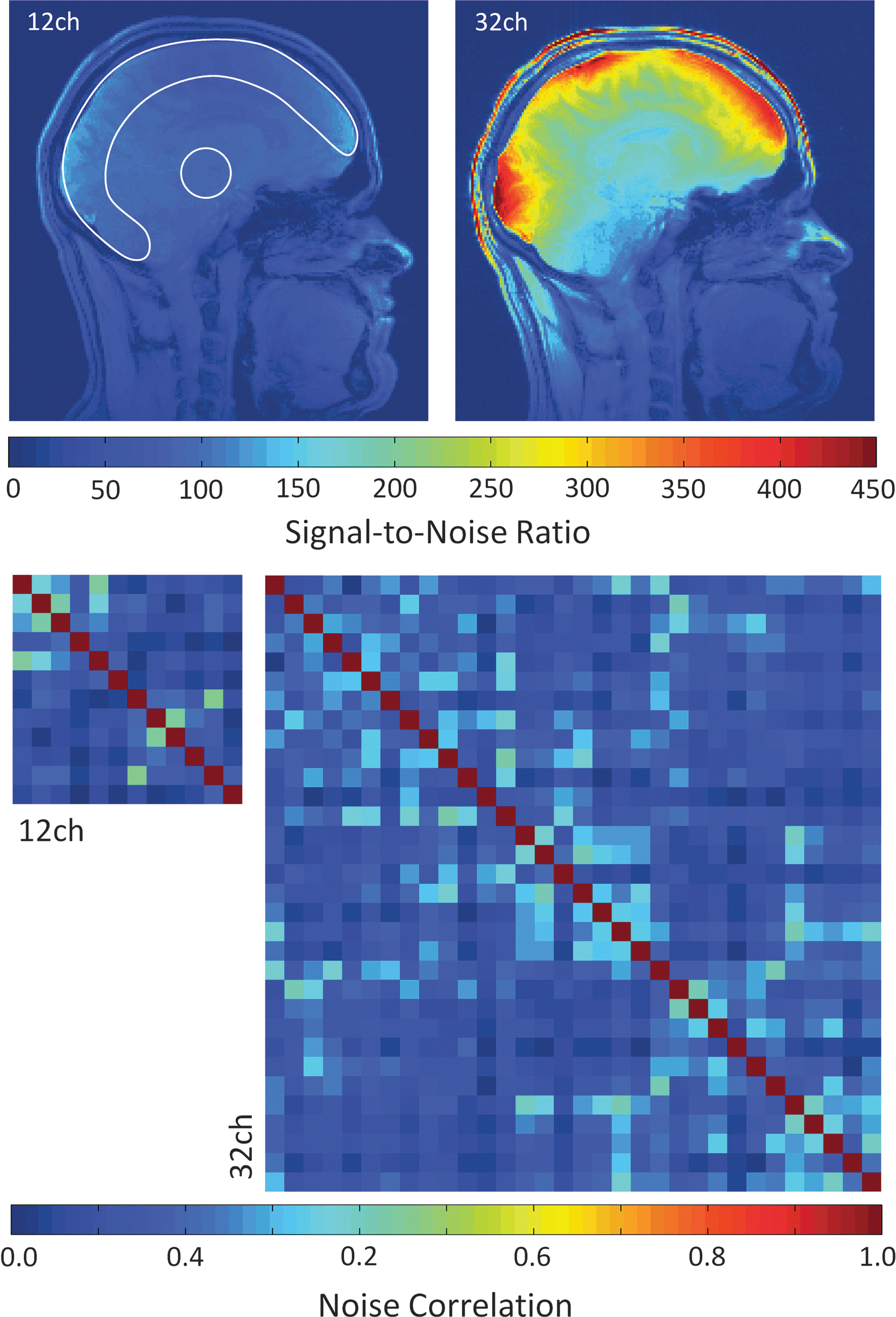
Pixel-wise signal-to-noise ratio (SNR) maps and noise correlation matrices from the 12 Channel (12Ch) and 32 Channel (32Ch) array coils. The 32Ch coil outperforms the 12Ch coil by a factor of 2.3×averaged over the given signal area. SNR from the peripheral cortex and the central brain region were obtained from the labeled regions of interest. The 32Ch coil shows a 1.25-fold and a 2.7-fold SNR improvement in the brain center and cortex, respectively. SNR increase in the corpus callosum region is 1.4 fold. SNR gain of the 32Ch coil can be attributed to both higher channel count and smaller helmet size. The 12Ch and 32Ch coil show average noise correlation (bottom row) of 12.3% and 9.7%, respectively.

Seed-based analysis

Figure 2 shows group-level results for the task-negative default networks (DMN and HCMN) from 32Ch and 12Ch array coils. Connections in all the seeds in the DMN (Fig. 2A) and HCMN (Fig. 2B) are significantly stronger in the 32Ch data set. Connections in left and right inferior temporal gyrus (ITG) extending to left and right parahippocampal gyrus (PHG), superior parietal cortex (SPC), and middle temporal gyrus (MTG) are more significant for DMN in the 32Ch_full>12Ch_full comparison (Table 2). Even with half the data set (Table 3), connections within the superior frontal gyrus (SFG), superior parietal lobule (SPL), and superior temporal gyrus (STG) were revealed with the 32Ch coil. Medial pre-frontal cortex (PFC) was significant even with 32Ch_half>12Ch_full contrast (Table 3).

FIG. 2.

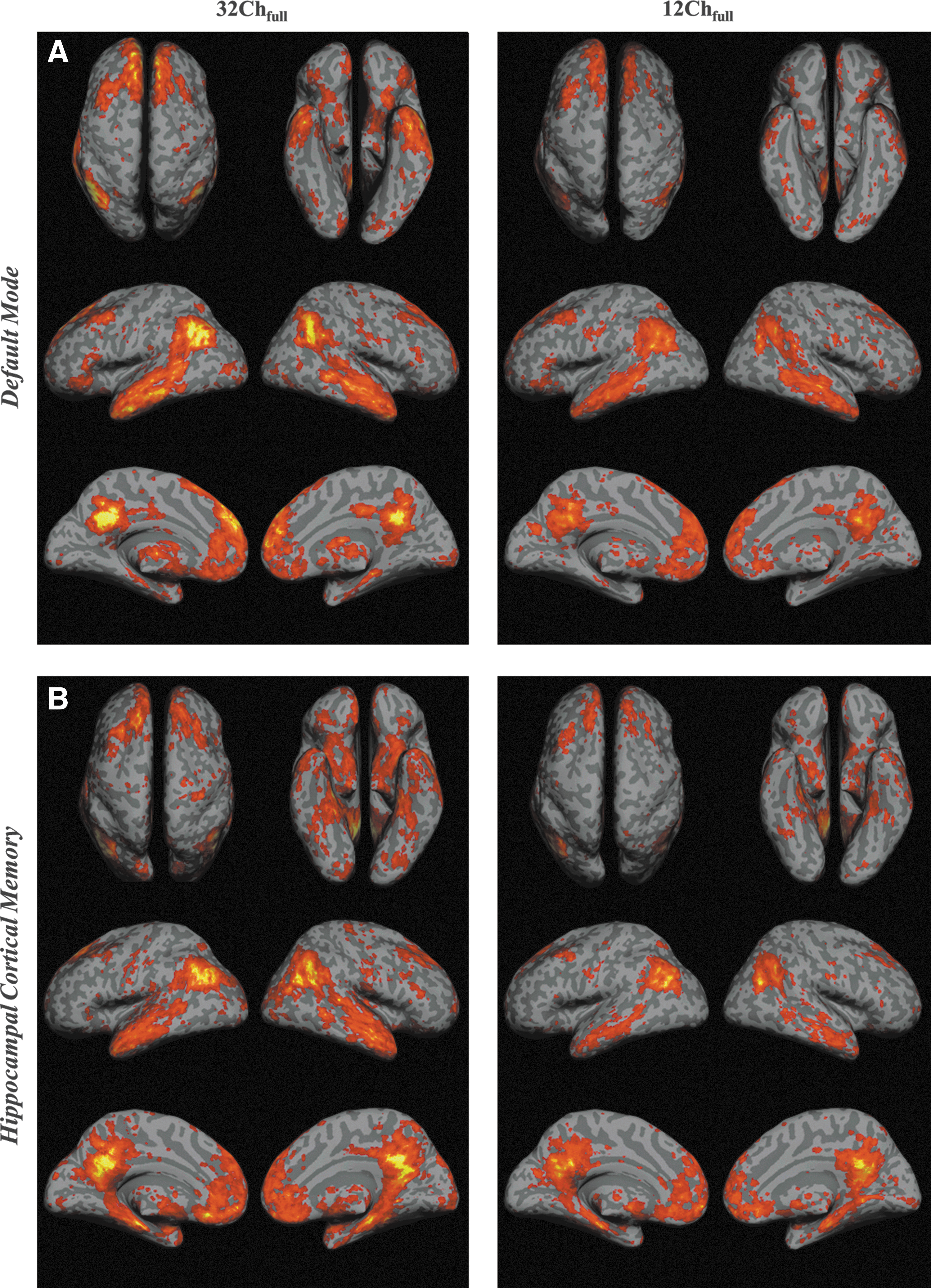
Statistical functional connectivity maps for (A) Default Mode and (B) Hippocampal Cortical Memory networks from 32Ch and 12Ch coils (second-level analysis, n=16 per group; whole-brain p_FDR-corr<0.05).

Table 2.

Positively Correlated Brain Regions for 32Ch_full>12Ch_full Contrast

Brain region	Brodmann area	Peak cluster	Voxels per cluster	T_max
	DMN
Left ITG	BA 20	−48 −6 −38	1016	6.35
Right SPC	BA 40	38 −50 28	161	5.32
Right SVC	BA 18	34 −76 −20	212	4.85
Right ITG	BA 20	40 −2 −48	244	4.38
Right MTG	BA 21	46 −4 −20	160	3.89
	HCMN
Left SVC	BA 18	−16 −100 18	255	6.51
Right MTG	BA 21	56 −12 6	614	5.15
OFC	BA 11	4 24 −22	263	4.99
Left MTG	BA 21	−56 −18 8	207	4.96
Right SVC	BA 18	24 −98 12	223	4.34
	DAN
Right DLPFC	BA 9	44 26 38	212	5.26
Right fusiform gyrus	BA 37	48 −50 −14	309	5.09
Right anterior PFC	BA 10	24 66 −10	144	4.88
Left fusiform gyrus	BA 37	−50 −56 −2	232	4.66
Left ITG	BA 20	−58 −32 −20	151	4.45
Left SPL	BA 7	−16 −48 50	114	4.06
	ECN
Right superior frontal gyrus	BA 8	40 26 38	439	8.73
Left MTG	BA 21	−58 −38 −8	285	5.32
Right MTG	BA 21	56 −44 0	262	4.88
Left DLPFC	BA 9	−36 2 32	225	4.76
Left SPC	BA 40	−52 −38 52	112	4.71
Left anterior PFC	BA 10	−20 62 10	254	4.50
Right anterior PFC	BA 10	36 40 2	138	4.33
Premotor cortex	BA 6	20 14 56	128	3.72
	SN
Left insular cortex	BA 13	−34 6 −2	917	7.07
Right insular cortex	BA 13	32 16 6	1243	6.15
Dorsal anterior cingulate cortex	BA 32	−4 26 24	920	5.51
Right anterior PFC	BA 10	34 3 8	143	4.91
Left DLPFC	BA 9	−26 38 20	507	4.86
Right DLPFC	BA 9	32 46 36	483	4.81
Left DLPFC	BA 9	−46 2 20	112	4.31
Left SPC	BA 40	−58 −38 40	182	4.03

Second-level group analysis, n=16 per group; cluster-level p_FWE-corr<0.05; height threshold: T=2.46; opposite contrast was not significant.

32Ch, 32 Channel; 12Ch, 12 Channel; ITG, inferior temporal gyrus; SVC, secondary visual cortex; MTG, middle temporal gyrus; OFC, orbitofrontal cortex; DLPFC, dorso lateral pre-frontal cortex; SPL, superior parietal lobule.

Table 3.

Positively Correlated Brain Regions for 32Ch_half>12Ch_full Contrast

Brain region	Brodmann area	Peak cluster	Voxels per cluster	T_max
	DMN
SFG	BA 8	14 40 44	98	4.72
SPL	BA 7	34 −64 50	91	4.43
Left superior temporal gyrus	BA 22	−54 −34 −2	106	4.16
	HCMN
Premotor cortex	BA 6	32 −6 54	95	5.08
OFC	BA 11	−6 16 −24	337	4.93
SFG	BA 8	0 34 40	480	4.72
Left DLPFC	BA 46	−44 32 10	102	4.56
Dorsal anterior cingulate cortex	BA 32	6 34 8	153	4.48
Right SPL	BA 7	42 −64 48	113	4.44
Right DLPFC	BA 46	44 46 12	130	4.24
	DAN
Right DLPFC	BA 9	48 36 26	107	6.41
Right anterior PFC	BA 10	38 56 14	210	5.12
Premotor cortex	BA 6	60 −14 16	116	4.83
Left SPL	BA 7	−24 −54 48	102	4.67
	ECN
Right inferior temporal gyrus	BA 20	54 −22 −18	127	6.78
Right anterior PFC	BA 10	40 26 36	789	6.76
Right insular cortex	BA 13	52 −12 2	175	5.69
Right anterior PFC	BA 10	34 52 −6	521	5.20
Right SPC	BA 40	52 −52 50	286	5.14
Left SFG	BA 8	−8 28 46	245	5.10
Left DLPFC	BA 9	−40 28 26	94	4.91
Right fusiform gyrus	BA 37	54 −44 −6	93	4.90
Left anterior PFC	BA 10	−4 46 8	130	4.22
Left SPC	BA 40	−36 −62 50	147	4.12
	SN
Right insular cortex	BA 13	36 −4 −6	146	6.30
Left insular cortex	BA 13	−32 −4 −12	215	5.82
SPL	BA 7	−2 −66 32	170	4.31

Second-level group analysis, n=16 per group; cluster-level p_FWE-corr<0.05; height threshold: T=2.46; opposite contrast was not significant.

SFG, superior frontal gyrus.

Group-level results for the task-positive networks (DAN, ECN, and SN) from 32Ch and 12Ch coils are shown in Figure 3. The 12Ch coil only revealed a small subset of the functional connectivity in DAN (Fig. 3A). Connections in dorso-lateral PFC (DLPFC), left and right fusiform gyrus, anterior PFC (APFC), ITG, and SPL were significantly stronger in the 32Ch data set (Table 2). The 32Ch_half>12Ch_full comparison (Table 3) revealed DLPFC, APFC, premotor cortex, and SPL.

FIG. 3.

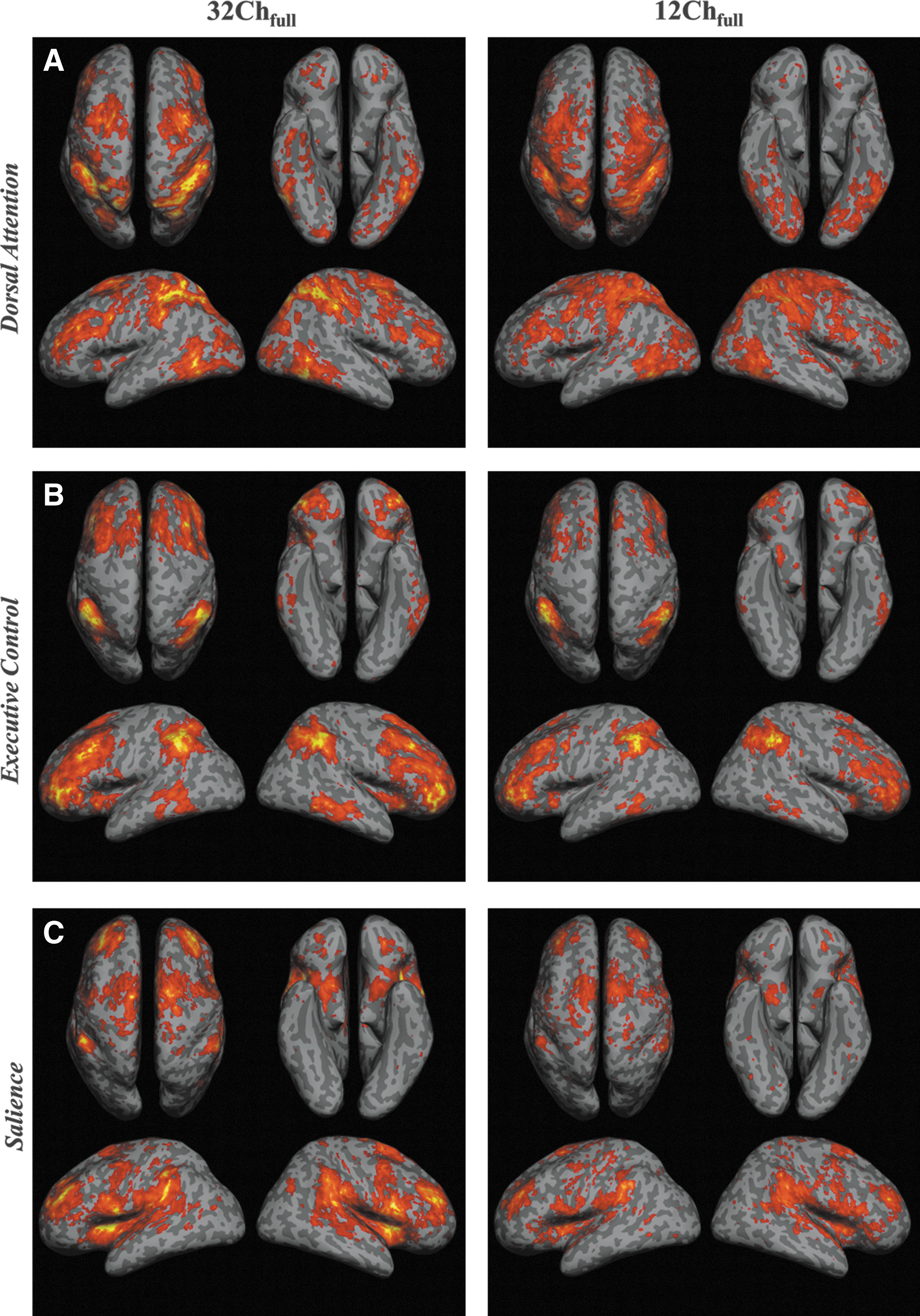
Statistical functional connectivity maps for (A) Dorsal Attetnion (B) Executive Control, and (C) Salience networks from 32Ch and 12Ch coils (second-level analysis, n=16 per group; whole-brain p_FDR-corr<0.05).

Figure 3B shows the functional connectivity correlation maps generated at the second level for ECN. The 32Ch_full>12Ch_full comparison (Table 2) revealed significant differences in SFG, left and right MTG, DLPFC, SPC, left and right APFC, and premotor cortex. The contrast 32Ch_half>12Ch_full (Table 3) also revealed significant differences, primarily in APFC.

Similar to all the networks mentioned earlier, the second-level analysis for SN (Fig. 3C) revealed only a smaller subset of the network for the 12Ch coil. Connections in left and right insular cortex were remarkably stronger with the 32Ch (both full and half data sets) in comparison to the 12Ch coil (Table 2). In addition, a 32Ch_full>12Ch_full comparison revealed dorsal anterior cingulate cortex (ACC), APFC, left and right DLPFC, and SPC (Table 3).

Representative examples for 32Ch_full>12Ch_full and 32Ch_half>12Ch_full contrasts are shown in Figure 4. For HCMN, connections in the left and right secondary visual cortex, orbitofrontal cortex, and left and right MTG were significantly more pronounced in the 32Ch_full>12Ch_full comparison (Fig. 4A). The entire ECN (dorsal medial PFC, left and right APFC, and left and right SPC) was significantly stronger with half the data set from the 32Ch coil (Fig. 4B).

FIG. 4.

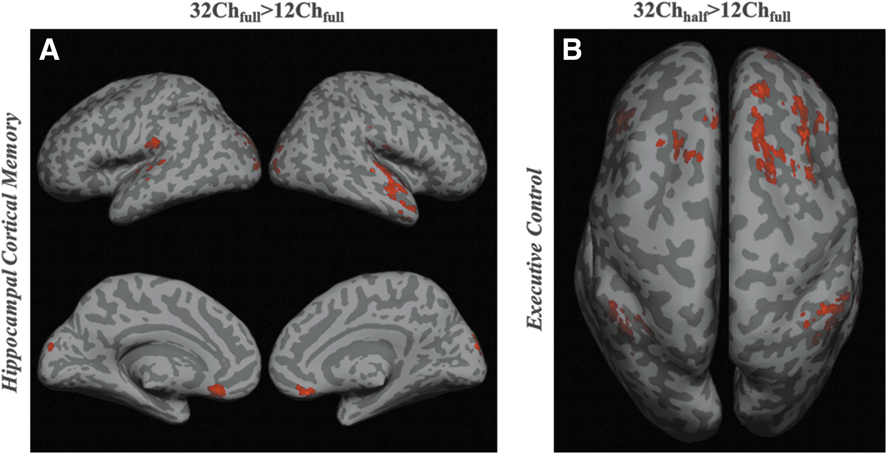
Representative examples from a task-negative and task-positive resting-state network for between-group comparisons from (A) 32Ch_full>12Ch_full and (B) 32Ch_half>12Ch_full contrasts (second-level analysis, n=16 per group; cluster-level p_FWE-corr<0.05; height threshold: T=2.46). (A) Connections in left and right temporal gyrii and medial prefrontal cortices of the default network are more significantly revealed with the 32Ch coil. (B) Entire executive control network (dorsal medial pre-frontal cortex, left and right anterior pre-frontal cortices, and left and right superior parietal cortices) is more significantly revealed with half the data set from the 32Ch coil.

For all the resting-state networks studied earlier, both 12Ch_full>32Ch_full and 12Ch_full>32Ch_half contrasts were not significant.

The sensitivity of the coils in deeper brain structures, the subcortical network of basal ganglia, was explored. Group-level results based on seed-to-voxel analysis demonstrated stronger functional connectivity in all the sub-cortical ROIs with 32Ch coil (Fig. 5). A 32Ch_full>12Ch_full comparison (whole-brain p_FDR-corr<0.05, cluster-level p_FWE-corr<0.05) revealed significantly stronger connections in bilateral pallidum, bilateral putamen, left precentral gyrus (BA 6), and STG (BA 22). ROI-to-ROI connectivity analysis for within-group comparisons (p_FDR-corr<0.05) revealed several interesting findings: (1) With thalamus as seed ROI, the 12Ch group failed to identify functional connectivity from relatively smaller structures such as substantia nigra and subthalamic nucleus; this was also the case when medial globus pallidus was chosen as the ROI; (2) with caudate (a part of the striatum) as seed ROI, correlations with medial globus pallidus were detected only by the 32Ch group; and (3) with lateral globus pallidus as seed ROI, the T scores for positive correlations from substantia nigra and subthalamic nucleus were 6.27 and 5.67 with the 32Ch coil; and 2.26 and 2.17 with the 12Ch coil.

FIG. 5.

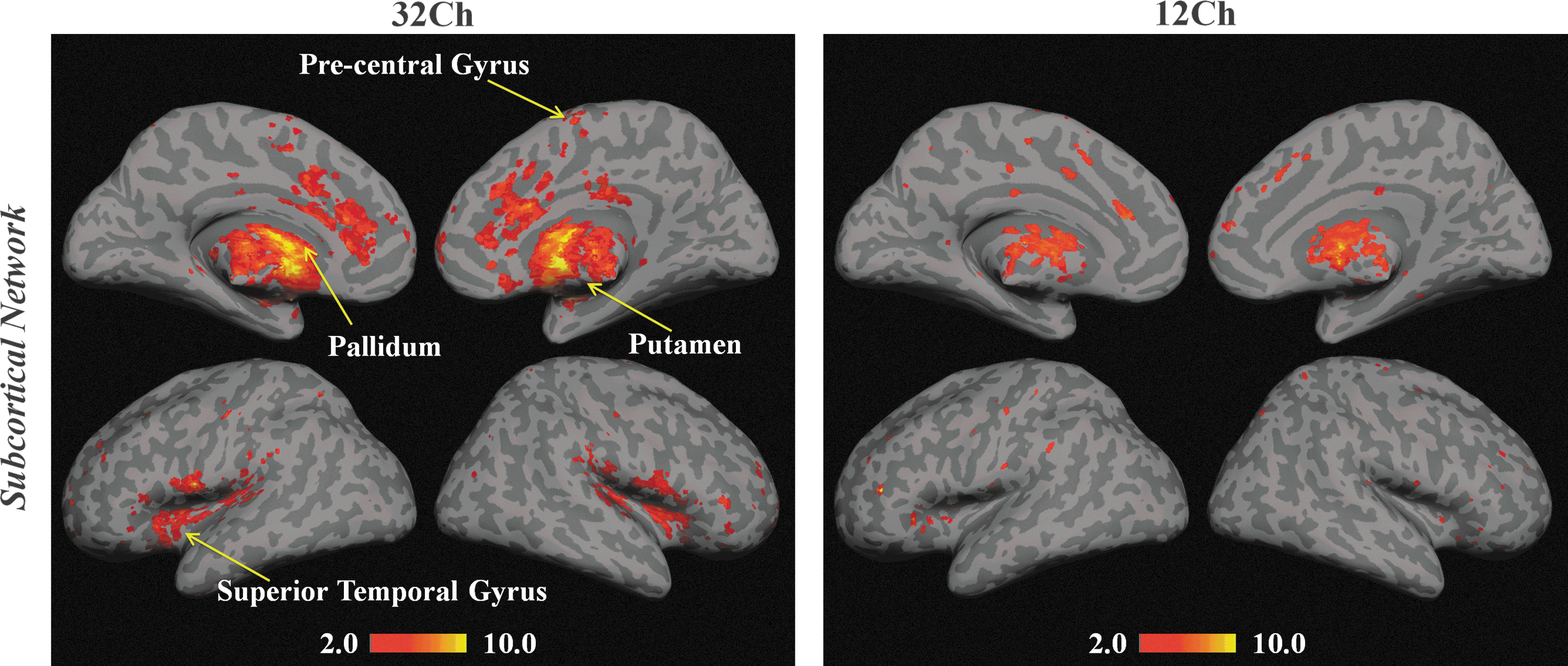
Statistical functional connectivity maps for the subcortical network from 32Ch and 12Ch coils (full data sets, second-level analysis, n=16 per group; whole-brain p_FDR-corr<0.05). Yellow arrows indicate the regions that are significantly different in the 32Ch_full>12Ch_full contrast (whole-brain p_FDR-corr<0.05, cluster-level p_FWE-corr<0.05).

Graph-theory-based analysis

Consistent with the small-world behavior of brain networks reported earlier (Achard and Bullmore, 2007), graph-theory-based analyses revealed monotonic increases in global and local efficiency as a function of cost in all brain networks (Fig. 6). As shown in Figure 6 (top row), the random graph had higher global efficiency than the lattice and vice versa, for costs (K) in the range 0≤K≤0.5. Brain networks (solid black line pertaining to our data represents data from all subjects for both 12Ch and 32Ch coils), however, in the cost range of 0.05≤K≤0.34, had a global efficiency that was greater than the lattice but less than the random graph, and a local efficiency which was greater than the random but less than the lattice graph (Fig. 6, bottom row). We, therefore, chose a cost threshold of 0.15 for our analyses. In the 32Ch_full>12Ch_full contrast, for analysis of global efficiency (p_FDR-corr<0.05), only left and right ACC (BA 33) surpassed the top 15% ROI-to-ROI connectivity (cost threshold of 0.15) from the network of all sources (84 Brodmann areas). Results from a network level analysis of cost are shown in Figure 7. Left and right ACC, left and right anterior entorhinal cortex (BA 34), and right perirhinal cortex (BA 35) surpassed the threshold (p_FDR-corr<0.05) for 32Ch_full>12Ch_full contrast (Fig. 7C). Even with half the data set from the 32Ch coil, an analysis of cost (p_FDR-corr<0.05) in the 32Ch_half>12Ch_full contrast revealed bilateral ACC. An analysis of local efficiency (p_FDR-corr<0.05) revealed right ACC and left PHG (BA 36). The opposite contrasts (12Ch_full>32Ch_full and 12Ch_full>32Ch_half) were not significant for all three measures. Global and local efficiency comparisons of full and half data sets from 32Ch, and full data sets from 12Ch coil at the cost threshold of 0.15 are summarized in Table 4. T values from 32Ch_full, 12Ch_full, and 32Ch_full>12Ch_full comparisons from the network-level analysis of cost (depicted in Fig. 7) for the top 15% ROI-to-ROI connectivity (p_FDR-corr<0.05) from all Brodmann areas (number of nodes=84, 16 subjects per group) are provided in Table 5. Brain regions provided in column 1 correspond to the ROIs represented as circles in Figure 7C (32Ch_full>12Ch_full comparison). Precisely, these are the brain regions that surpassed the threshold (p_FDR-corr<0.05) for 32Ch_full>12Ch_full contrast during the network-level analysis of cost.

FIG. 6.

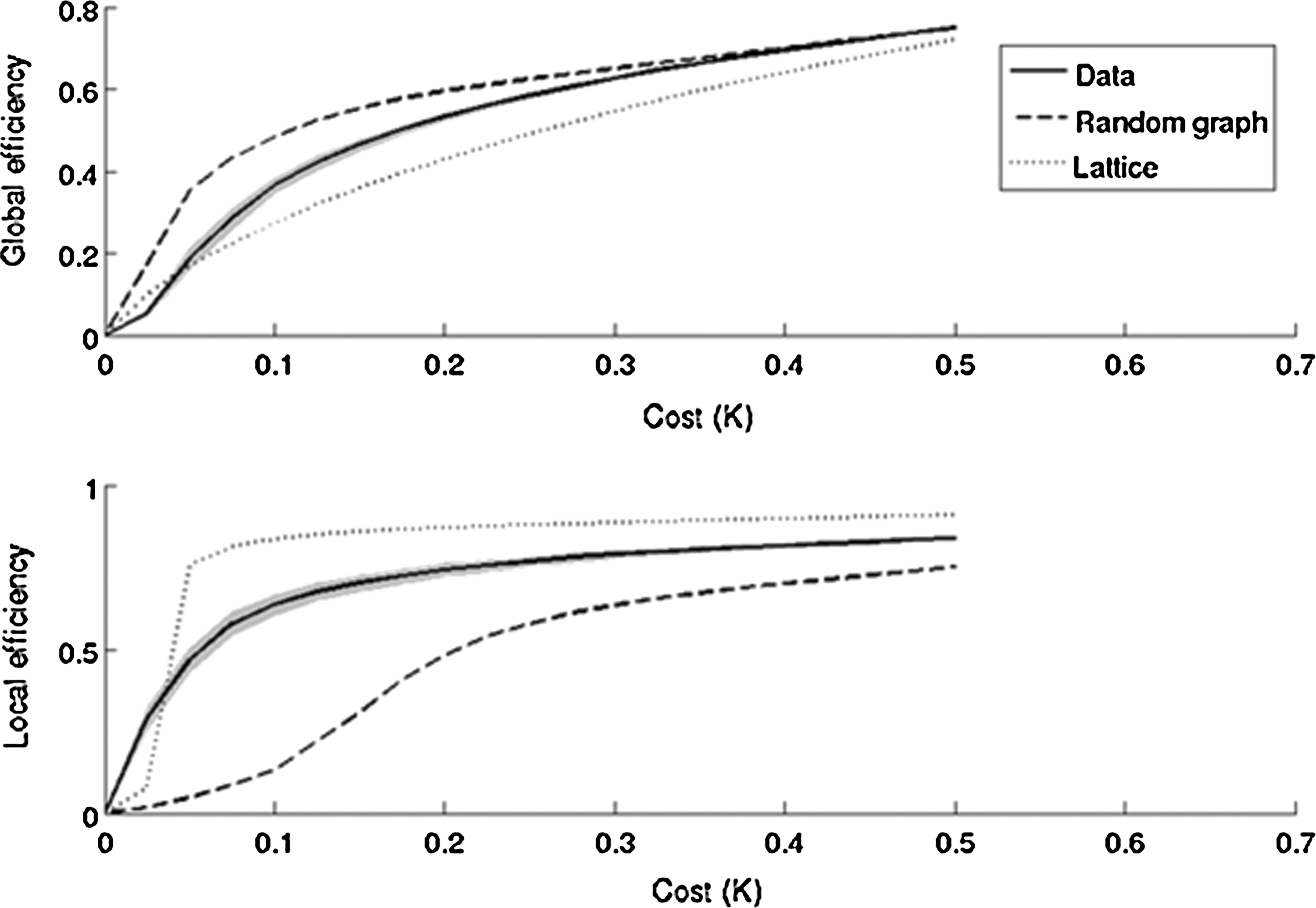
Global and local efficiency (y-axis) as a function of cost (x-axis) for a random graph, a regular lattice, and brain networks. On average, over all subjects in both 12Ch and 32Ch groups, brain networks have efficiency curves located between the limiting cases of random and lattice topology. Solid black line represents data from all subjects for both 12Ch and 32Ch coils.

FIG. 7.

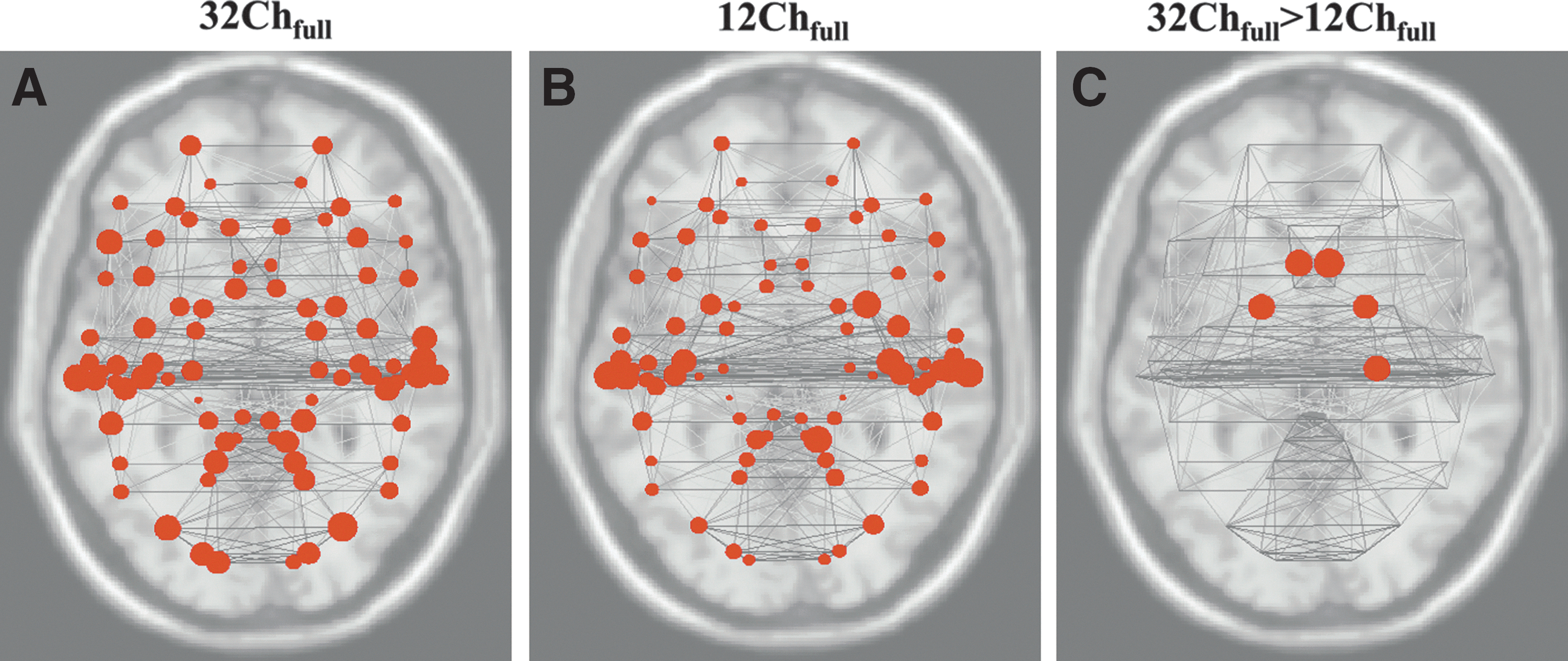
Graph visualization of the network-level analysis of cost for the top 15% region of interest to region of interest connectivity (p_FDR-corr<0.05) from all Brodmann areas for (A) 32Ch_full, (B) 12Ch_full, and (C) 32Ch_full >12Ch_full contrasts (number of nodes=84; 16 subjects per group). Circle sizes represent T values.

Table 4.

Global and Local Efficiency Comparisons of 32 Channel and 12 Channel Coils (Graph Theory Analysis), for the Top 15% Region of Interest-to-Region of Interest Connectivity (p_FDR _-corr<0.05), from All Brodmann Areas (Number of Nodes=84; 16 Subjects per Group)

Coil	Global efficiency	Local efficiency
32Ch_full	0.471	0.717
32Ch_half	0.455	0.697
12Ch_full	0.459	0.688
p_FDR (32Ch_full>12Ch_full)	0.056	0.034
p_FDR (12Ch_full>32Ch_full)	n.s.	n.s.

n.s., not significant.

Table 5.

T Values from 32Ch_full, 12Ch_full, and 32Ch_full>12Ch_full Comparisons from the Network-Level Analysis of Cost (Depicted in Figure 7) for the Top 15% Region of Interest to Region of Interest Connectivity (p_FDR _-corr <0.05) from All Brodmann Areas (Number of Nodes=84; 16 Subjects per Group)

	T scores
Brain region	32Ch	12Ch	32Ch>12Ch
Left anterior entorhinal cortex	9.73	6.21	3.18
Right anterior entorhinal cortex	9.68	8.82	2.99
Right perirhinal cortex	8.45	5.83	3.17
Right ACC	6.01	3.31	3.58
Left ACC	4.70	3.57	3.26

Brain regions provided in column 1 correspond to the regions of interest represented as circles in Figure 7C (32Ch_full>12Ch_full comparison). Precisely, these are the brain regions that surpassed the threshold (p_FDR-corr<0.05) for 32Ch_full>12Ch_full contrast during the network-level analysis of cost.

ACC, anterior cingulate cortex.

Discussion

Multichannel arrays offer close head fittings, impressive increases in the image SNR, especially in cortical areas, and remarkable accelerated imaging capabilities. Due to these advantages, multichannel array coils have recently become widely available not only as experimental devices (Keil et al., 2011, 2012; Wiggins et al., 2006) but also as clinical research tools (Knake et al., 2005; Parikh et al., 2011; Raoult et al., 2011). In this study, task-positive (dorsal attention, executive control, and salience), task-negative (default mode and hippocampal cortical memory), and subcortical (basal ganglia) resting-state networks were assessed to examine whether increases in tSNR with the additive coil sensitivity of a 32Ch brain array can translate to higher functional connectivity detectability when compared with a 12Ch coil. Our findings, from both seed-based and graph-theory-based functional connectivity analyses methods, demonstrated that the 32Ch brain array revealed stronger connections (32Ch_full>12Ch_full contrast) in all the resting-state networks studied. Further, precise localization of functional connectivity mapping was also observed using the 32Ch coil, when fMRI time-series acquisition time was reduced to half of its original duration (∼3 min vs. 6 min scan).

The increased SNR capabilities of the 32Ch coil in combination with the high-resolution acquisition scheme enabled us to identify the resting-state networks at the group level (16 subjects) in greater detail compared with the 12Ch coil. The core of the DMN, according to the literature, is formed by PCC, MPFC, left and right LPC, and left and right inferior temporal cortices (Fox et al., 2005). The fact that the ITG was detected to a significantly stronger extent by the 32Ch coil reflects one of the major limitations of the 12Ch coil in terms of SNR at higher-resolution acquisitions. Further, connections from relatively smaller brain structures, such as PHG, which are not typically identified even at the group level by the 12Ch coil, were detected by the 32Ch coil in our group data. This was particularly accurate in the HCMN comparison between the two coils. Significantly, a better detection of connections between hippocampus and orbitofrontal gyrus offers a clear advantage for using 32Ch coil in studies involving hippocampal–orbitofrontal connectivity, particularly in the context of epilepsy (Catenoix et al., 2005). For the DAN, at which frontal eye field, intraparietal sulcus, and MTG comprise the core signal components (Fox et al., 2005), functional connectivity was extremely weak, particularly in the frontal and parietal cortices when the data from the 12Ch coil were used. Core signal components of the ECN, inferior, middle and superior frontal gyrii (Seeley et al., 2007), as well as the insula and cingulate cortex, which comprise the SN (Taylor et al., 2009), were significantly stronger for the 32Ch_full>12Ch_full comparison. Impairments in the executive network have been suggested in social anxiety disorders (Qiu et al., 2011), where the 32Ch coil could offer a clear benefit. The right insular cortex even surpassed a much stronger threshold (whole-brain p_FDR-corr<0.05) for the 32Ch_full>12Ch_full contrast. This is of particular significance in light of previous research (Sridharan et al., 2008) and, more recently, in addiction studies (Sutherland et al., 2012), which showed that the right-fronto insular cortex is a network hub that plays a critical role in initiating the spontaneous switching between the task-positive (ECN) and task-negative (DMN) networks (Honey et al., 2007).

To further explore the CNR advantages of the 32Ch, we have investigated functional connectivity in the deeper structures of the thalamus and basal ganglia (i.e., sub-cortical network). Between-group comparisons (32Ch_full>12Ch_full) revealed significantly stronger connections in bilateral pallidum, bilateral putamen, left pre-central gyrus, STG, and within the basal ganglia structures, which is consistent with recent reports that use the 16Ch coil at 7T (Lenglet et al., 2012). Further, the 12Ch coil failed to identify connections with substantia nigra and subthalamic nucleus, which are relatively smaller structures and typically excluded from analysis when low-resolution acquisition (3×3×3 mm³) is employed (Di Martino et al., 2008). This result is in agreement with the SNR performance shown in Figure 1, where the 32Ch array outperforms the 12Ch coil in SNR by a factor of 1.25×and 2.7×at the central and peripheral cortex, respectively. By increasing the channel count of a head array coil from 12 to 32, an overall 1.8-fold SNR improvement can be expected, while main SNR gain contribution is expected to occur at the peripheral regions (e.g., brain cortex), while the central SNR will remain relatively the same (Wiesinger et al., 2004). However, the product-available 32Ch head array coils provide a tighter fit compared with dimensionally larger designed 12Ch coils. For the arrays under study in the present work (32Ch and 12Ch coils), since the 32Ch array is constructed on a tighter fitting helmet than the 12Ch (or most other arrays), it also enjoys a sensitivity benefit from the closer proximity between receive element and brain. This benefit extends to deep structures as well as the superficial cortex. Increases in SNR obtained from 32Ch coils can then be traded off for acquisitions with a higher spatial resolution, which becomes particularly important for fMRI.

A graph-theory-based analyses revealed a significantly higher overall global efficiency of nodes (i.e., stronger connections) with the 32Ch coil compared with the 12Ch coil, particularly in ACC. There is converging evidence from recent publications that functional connectivity in ACC changes through brain maturation in healthy subjects (Kelly et al., 2009) and also in attention deficit hyperactivity disorder patients (Qiu et al., 2010). A significantly higher local efficiency of PHG revealed by the 32Ch coil compared with the 12Ch coil showed that this region formed a strong/well-connected network with its neighbors. In the 32Ch_full>12Ch_full contrast, there is a trend (p=0.056) toward a higher global efficiency. This could be indicative of the sensitivity of the 32Ch coil to detect long-range connections. In particular, differences in global efficiency between networks are typically related to differences in the amount of long-range connectivity within the network for small-world networks. Similarly, a significantly different local efficiency (p=0.034) in the 32Ch_full>12Ch_full contrast indicates the sensitivity of the 32Ch coil to detect short-range connections (because short-range connections are associated to a higher local efficiency, that is, how well its neighbors are still connected if we eliminate this node). Since these two metrics are vital to understanding the brain's ability to integrate information at the global level (i.e., functional integration) and cluster level (i.e., functional segregation) (Rubinov and Sporns, 2010), the 32Ch coil would prove more beneficial to elucidate the intricacies of brain networks. Cost advantages of the 32Ch coil are depicted in Figure 7, which provides a graph visualization of the network-level analysis of cost for the top 15% ROI-to-ROI connectivity (p_FDR-corr<0.05) from all Brodmann areas (number of nodes=84; 16 subjects per group). A network-level analysis of cost revealed that connections in ACC are significantly stronger in both 32Ch_full>12Ch_full and 32Ch_half>12Ch_full comparisons. Perirhinal, entorhinal, and parahippocampal cortices are a part of the medial temporal lobe (MTL) and based on our results, especially from graph-theory-based analysis, we suggest that the 32Ch coil would be better suited for studies involving MTL pathologies such as Alzheimer's disease and epilepsy. A significantly higher functional connectivity, observed in inferior/medial temporal regions with the 32Ch coil, consistently in DMN, HCMN, DAN, and ECN, reiterates this benefit.

In this study, time-series data were acquired in a relatively higher spatial resolution (2×2×2 mm³) compared with a typically employed low resolution (3×3×4 mm³) in fMRI, based on findings from a recent work (Triantafyllou et al., 2011) which demonstrated that array coils provide biggest increases in tSNR at high spatial resolutions (small voxel size). In our resting-state protocol, we chose to acquire data at a 2 mm isotropic voxel size to utilize the benefits of the multichannel array as well as to increase the spatial specificity and localization of the networks and to minimize partial volume effects and physiological noise contamination.

In fMRI studies, events/blocks are repeated several times so that task-related activations are detected more reliably. This often leads to long experiments inducing subject fatigue and/or head motion, the levels of which may confound the results. Moreover, such long experiments might not be feasible in specific subject populations, such as pediatrics or patients. Typically, reduction in scan time is possible only at the expense of SNR, but not necessarily if one could capitalize on the increased sensitivity afforded by multichannel arrays or high magnetic field strength. In this study, we demonstrate that increases in tSNR offered by the 32Ch coil can also translate to reductions in scan time, that is, less number of time points per functional run or ultimately less runs of the same experiment in fMRI. In our resting-state experiments, particularly, connections within SFG were significantly stronger in the 32Ch_half>12Ch_full comparison for both DMN and HCMN, as were DLPFC, APFC, premotor cortex, and SPL in DAN (task-positive network). Similarly, the ECN and the SN revealed, within a network, significantly strong connections with half the duration of the 32Ch fMRI acquisition. Similarly, this can also be translated to power calculations for group fMRI studies (Mumford and Nichols, 2008), by having a lesser sample size or preventing the collection of additional data that will have a little impact on power.

The signal dynamic range of the 32Ch receive coil in the brain is approximately twice as that of the 12Ch head coil. This steeply varying spatial sensitivity profile of the small receiver coil elements of the 32Ch array has two important consequences. First, it causes a non-uniform detection sensitivity that spatially modulates the ability to detect BOLD fluctuations. This adds to other sources of BOLD detection variation such as biological effects (differences in cerebral blood flow and cerebral blood volume responses and differing hemodynamic response functions) as well as other instrumental effects such as imperfect B₀ shimming (which creates T2* variation and subsequently degrades the optimality of the TE setting). The effect of the coil sensitivity can be easily visualized by creating a tSNR map of the resting brain. Alternatively, the BOLD sensitivity map (Deichmann et al., 2002; Gorno-Tempini et al., 2002) includes this information through the explicit incorporation of the image signal intensity profile.

The most problematic issue with regard to the spatially varying reception is the increased sensitivity to motion. Motion effects in the resting-state have well-known detrimental consequences (Power et al., 2012; Satterthwaite et al., 2012; Van Dijk et al., 2012), which are exacerbated when parallel imaging acceleration is used to incorporate reference data or coil sensitivity maps are taken at the beginning of the scan. Movement then leads to changing levels of residual aliasing in the time series. Even for non-accelerated imaging, problems are derived from the spatially varying signal levels that are present in an array coil image. Even after perfect rigid-body alignment (motion correction), the signal time course in a given brain structure remains modulated by the motion of that structure through the steep sensitivity gradient. Motion correction (prospective or retrospective) brings brain structures into alignment across the time series but does not alter their intensity changes that are incurred from movement through the coil profiles of the fixed-position coils. This effect can be partially removed by regression of the residuals of the motion parameters; a step that has been shown to be very successful in removing nuisance variance in ultra-high field array coil data (Hutton et al., 2011). An improved strategy might be to model and remove the expected nuisance intensity changes by using the motion parameters and the coil sensitivity map.

As already demonstrated, the achievable SNR improvements of the 32Ch over the 12Ch head coil not only at the cortex but also at deeper brain areas are due to the increased number of elements and the tight-fitting helmet design of the 32Ch array, respectively. However, in practice, potentially two limitations are associated to the tight-fitting design: (1) not all head sizes fit in the helmet, and (2) there is no room for the commonly used MRI compatible headphones with big earmuffs. For the latter, alternative solutions should be considered; for example, inner-ear headphones or ultra-slim earmuffs that are available in the market.

Conclusions

In this work, we demonstrated that the improved signal detection capability of the 32Ch coil and its higher sensitivity result in increased functional connections and stronger correlation strengths, which potentially offer an opportunity for smaller sample size in group-level statistics and, therefore, prevent additional data collection. Our characterization of multichannel arrays was performed on the particular design and coil manufacturer. Other multichannel arrays might offer a different degree of sensitivity in the cortical brain areas compared with deeper structures due to a variability in the design configuration.

Footnotes

Acknowledgments

The authors would like to thank the Athinoula A. Martinos Imaging Center at McGovern Institute for Brain Research, Massachusetts Institute of Technology, for funding and Larry Wald for helpful comments on this article.

Author Disclosure Statement

No competing financial interests exist.

References

Achard

, Bullmore

. 2007. Efficiency and cost of economical brain functional networks. PLoS Comput Biol, 3:e17.

Ashburner

, Friston

. 2005. Unified segmentation. Neuroimage, 26:839–851.

Behzadi

, Restom

, Liau

, Liu

. 2007. A component based noise correction method (CompCor) for BOLD and perfusion based fMRI. Neuroimage, 37:90–101.

Biswal

, Yetkin

, Haughton

, Hyde

. 1995. Functional connectivity in the motor cortex of resting human brain using echo-planar MRI. Magn Reson Med, 34:537–541.

Bullmore

, Sporns

. 2009. Complex brain networks: graph theoretical analysis of structural and functional systems. Nature reviews. Neuroscience, 10:186–198.

Catenoix

, Magnin

, Guenot

, Isnard

, Mauguiere

, Ryvlin

. 2005. Hippocampal-orbitofrontal connectivity in human: an electrical stimulation study. Clin Neurophysiol: official journal of the International Federation of Clinical Neurophysiology, 116:1779–1784.

Chai

, Castanon

, Ongur

, Whitfield-Gabrieli

. 2012. Anticorrelations in resting state networks without global signal regression. Neuroimage, 59:1420–1428.

Corbetta

, Shulman

. 2002. Control of goal-directed and stimulus-driven attention in the brain. Nature reviews. Neuroscience, 3:201–215.

Deichmann

, Josephs

, Hutton

, Corfield

, Turner

. 2002. Compensation of susceptibility-induced BOLD sensitivity losses in echo-planar fMRI imaging. Neuroimage, 15:120–135.

10.

Di Martino

, Scheres

, Margulies

, Kelly

, Uddin

, Shehzad

, Biswal

, Walters

, Castellanos

, Milham

. 2008. Functional connectivity of human striatum: a resting state FMRI study. Cereb Cortex, 18:2735–2747.

11.

Fox

, Snyder

, Vincent

, Corbetta

, Van Essen

, Raichle

. 2005. The human brain is intrinsically organized into dynamic, anticorrelated functional networks. Proc Natl Acad Sci U S A, 102:9673–9678.

12.

Wiggins

, Wald

, Sodickson

. 2010. Performance evaluation of a 32-element head array with respect to the ultimate intrinsic SNR. NMR Biomed, 23:142–151.

13.

Friston

. 2007. Statistical Parametric Mapping: The Analysis of Funtional Brain Images. Amsterdam, Boston: Elsevier/Academic Press.

14.

Gorno-Tempini

, Hutton

, Josephs

, Deichmann

, Price

, Turner

. 2002. Echo time dependence of BOLD contrast and susceptibility artifacts. Neuroimage, 15:136–142.

15.

Greicius

, Krasnow

, Reiss

, Menon

. 2003. Functional connectivity in the resting brain: a network analysis of the default mode hypothesis. Proc Natl Acad Sci U S A, 100:253–258.

16.

Hayes

, Axel

. 1985. Noise performance of surface coils for magnetic resonance imaging at 1.5 T. Med Phys, 12:604–607.

17.

Honey

, Kotter

, Breakspear

, Sporns

. 2007. Network structure of cerebral cortex shapes functional connectivity on multiple time scales. Proc Natl Acad Sci U S A, 104:10240–10245.

18.

Hutton

, Josephs

, Stadler

, Featherstone

, Reid

, Speck

, Bernarding

, Weiskopf

. 2011. The impact of physiological noise correction on fMRI at 7 T. Neuroimage, 57:101–112.

19.

Keil

, Alagappan

, Mareyam

, McNab

, Fujimoto

, Tountcheva

, Triantafyllou

, Dilks

, Kanwisher

, Lin

, Grant

, Wald

. 2011. Size-optimized 32-channel brain arrays for 3 T pediatric imaging. Magn Reson Med, 66:1777–1787.

20.

Keil

, Blau

, Biber

, Hoecht

, Tountcheva

, Setsompop

, Triantafyllou

, Wald

. 2012. A 64-channel 3T array coil for accelerated brain MRI. Magn Reson Med. official journal of the Society of Magnetic Resonance in Medicine/Society of Magnetic Resonance in Medicine.

21.

Kellman

, McVeigh

. 2005. Image reconstruction in SNR units: a general method for SNR measurement. Magn Reson Med: official journal of the Society of Magnetic Resonance in Medicine/Society of Magnetic Resonance in Medicine, 54:1439–1447.

22.

Kelly

, Di Martino

, Uddin

, Shehzad

, Gee

, Reiss

, Margulies

, Castellanos

, Milham

. 2009. Development of anterior cingulate functional connectivity from late childhood to early adulthood. Cereb Cortex, 19:640–657.

23.

Knake

, Triantafyllou

, Wald

, Wiggins

, Kirk

, Larsson

, Stufflebeam

, Foley

, Shiraishi

, Dale

others2005. 3T phased array MRI improves the presurgical evaluation in focal epilepsies: a prospective study. Neurology, 65:1026–1031.

24.

Lancaster

, Woldorff

, Parsons

, Liotti

, Freitas

, Rainey

, Kochunov

, Nickerson

, Mikiten

, Fox

. 2000. Automated Talairach atlas labels for functional brain mapping. Hum Brain Mapp, 10:120–131.

25.

Lenglet

, Abosch

, Yacoub

, De Martino

, Sapiro

, Harel

. 2012. Comprehensive in vivo mapping of the human basal ganglia and thalamic connectome in individuals using 7T MRI. PLoS One, 7:e29153.

26.

Maldjian

, Laurienti

, Burdette

. 2004. Precentral gyrus discrepancy in electronic versions of the Talairach atlas. Neuroimage, 21:450–455.

27.

Maldjian

, Laurienti

, Kraft

, Burdette

. 2003. An automated method for neuroanatomic and cytoarchitectonic atlas-based interrogation of fMRI data sets. Neuroimage, 19:1233–1239.

28.

Mumford

, Nichols

. 2008. Power calculation for group fMRI studies accounting for arbitrary design and temporal autocorrelation. Neuroimage, 39:261–268.

29.

Parikh

, Sandhu

, Blackham

, Coffey

, Hsu

, Liu

, Jesberger

, Griswold

, Sunshine

. 2011. Evaluation of image quality of a 32-channel versus a 12-channel head coil at 1.5T for MR imaging of the brain. AJNR Am J Neuroradiol, 32:365–373.

30.

Power

, Barnes

, Snyder

, Schlaggar

, Petersen

. 2012. Spurious but systematic correlations in functional connectivity MRI networks arise from subject motion. Neuroimage, 59:2142–2154.

31.

Qiu

, Liao

, Ding

, Feng

, Zhu

, Nie

, Zhang

, Chen

, Gong

. 2011. Regional homogeneity changes in social anxiety disorder: a resting-state fMRI study. Psychiatry Res, 194:47–53.

32.

Qiu

, Ye

, Li

, Liu

, Xie

, Wang

. 2010. Changes of brain structure and function in ADHD children. Brain Topogr, 24:243–252.

33.

Raoult

, Petr

, Bannier

, Stamm

, Gauvrit

, Barillot

, Ferre

. 2011. Arterial spin labeling for motor activation mapping at 3T with a 32-channel coil: reproducibility and spatial accuracy in comparison with BOLD fMRI. Neuroimage, 58:157–167.

34.

Roemer

, Edelstein

, Hayes

, Souza

, Mueller

. 1990. The NMR phased array. Magn Reson Med: official journal of the Society of Magnetic Resonance in Medicine/Society of Magnetic Resonance in Medicine, 16:192–225.

35.

Rubinov

, Sporns

. 2010. Complex network measures of brain connectivity: uses and interpretations. Neuroimage, 52:1059–1069.

36.

Satterthwaite

, Wolf

, Loughead

, Ruparel

, Elliott

, Hakonarson

, Gur

. 2012. Impact of in-scanner head motion on multiple measures of functional connectivity: relevance for studies of neurodevelopment in youth. Neuroimage, 60:623–632.

37.

Seeley

, Menon

, Schatzberg

, Keller

, Glover

, Kenna

, Reiss

, Greicius

. 2007. Dissociable intrinsic connectivity networks for salience processing and executive control. J Neurosci: the official journal of the Society for Neuroscience, 27:2349–2356.

38.

Sridharan

, Levitin

, Menon

. 2008. A critical role for the right fronto-insular cortex in switching between central-executive and default-mode networks. Proc Natl Acad Sci U S A, 105:12569–12574.

39.

Sutherland

, McHugh

, Pariyadath

, Stein

. 2012. Resting state functional connectivity in addiction: lessons learned and a road ahead. Neuroimage, 62:2281–2295.

40.

Taylor

, Seminowicz

, Davis

. 2009. Two systems of resting state connectivity between the insula and cingulate cortex. Hum Brain Mapp, 30:2731–2745.

41.

Triantafyllou

, Polimeni

, Wald

. 2011. Physiological noise and signal-to-noise ratio in fMRI with multi-channel array coils. Neuroimage, 55:597–606.

42.

van der Kouwe

, Benner

, Fischl

, Schmitt

, Salat

, Harder

, Sorensen

, Dale

. 2005. On-line automatic slice positioning for brain MR imaging. Neuroimage, 27:222–230.

43.

Van Dijk

, Hedden

, Venkataraman

, Evans

, Lazar

, Buckner

. 2010. Intrinsic functional connectivity as a tool for human connectomics: theory, properties, and optimization. J Neurophysiol, 103:297–321.

44.

Van Dijk

, Sabuncu

, Buckner

. 2012. The influence of head motion on intrinsic functional connectivity MRI. Neuroimage, 59:431–438.

45.

Vincent

, Kahn

, Snyder

, Raichle

, Buckner

. 2008. Evidence for a frontoparietal control system revealed by intrinsic functional connectivity. J Neurophysiol, 100:3328–3342.

46.

Whitfield-Gabrieli

, Nieto-Castanon

. 2012. Conn: a functional connectivity toolbox for correlated and anticorrelated brain networks. Brain Connect, 2:125–141.

47.

Wiesinger

, Boesiger

, Pruessmann

. 2004. Electrodynamics and ultimate SNR in parallel MR imaging. Magn Reson Med: official journal of the Society of Magnetic Resonance in Medicine/Society of Magnetic Resonance in Medicine, 52:376–390.

48.

Wiggins

, Polimeni

, Potthast

, Schmitt

, Alagappan

, Wald

. 2009. 96-Channel receive-only head coil for 3 Tesla: design optimization and evaluation. Magn Reson Med, 62:754–762.

49.

Wiggins

, Triantafyllou

, Potthast

, Reykowski

, Nittka

, Wald

. 2006. 32-channel 3 Tesla receive-only phased-array head coil with soccer-ball element geometry. Magn Reson Med: official journal of the Society of Magnetic Resonance in Medicine/Society of Magnetic Resonance in Medicine, 56:216–223.

50.

Zhang

, Raichle

. 2010. Disease and the brain's dark energy. Nature reviews. Neurology, 6:15–28.