Matching Structural,Effective,and Functional Connectivity: A Comparison Between Structural Equation Modeling and Ancestral Graphs

Abstract

In this study, we examined the accuracy of ancestral graphs (AGs) to study effective connectivity in the brain. Unlike most other methods that estimate effective connectivity, an AG is able to explicitly model missing brain regions in a network model. We compared AGs with the conventional structural equation models (SEM). We used both methods to estimate connection strengths between six regions of interest of the visual cortex based on functional magnetic resonance imaging data of a motion perception task. In order to examine which method is more accurate to estimate effective connectivity, we compared the connection strengths of the AG and SEM models with connection probabilities resulting from probabilistic tractography obtained from diffusion tensor images. This was done by correlating the connection strengths of the best fitting AG and SEM models with the connection probabilities of the probabilistic tractography models. We show that, in general, AGs result in more accurate models to estimate effective connectivity than SEM. The reason for this is that missing regions are taken into account when modeling with AG but not when modeling with SEM: AG can be used to explicitly test the assumption of missing regions. If the set of regions is complete, SEM and AG perform about equally well.

Introduction

The brain is a network of brain regions that are connected by anatomical tracts (Rubinov and Sporns, 2010; Van den Heuvel and Hulshoff Pol, 2010). Brain connectivity can be studied at a structural (anatomical) and a functional level in a noninvasive way by magnetic resonance imaging (MRI) techniques. At the structural level, connectivity refers to the anatomical links of the brain that are made up of white matter tracts which can be modeled by diffusion tensor imaging (DTI) (Guye et al., 2008; Johansen-Berg and Behrens, 2006; Rykhlevskaia et al., 2008; Tournier et al., 2011). At the functional level, connectivity reflects statistical associations (e.g., correlations) between regions based on indirect detection of neural activity through blood oxygen level-dependent (BOLD) signals measured with functional MRI (fMRI) (Bullmore and Sporns, 2009; Friston et al., 2003; He and Evans, 2010).

Connectivity at the functional level can be further divided into functional and effective connectivity. Functional connectivity is defined as the (temporal) correlation between different brain regions, whereas effective connectivity refers to the influence that one brain area exerts on another (Büchel and Friston, 1997; Bullmore and Sporns, 2009; Friston, 2011; Telesford et al., 2011). In contrast to functional connectivity, where connections are undirected, effective connectivity contains directed connections, implying a causal relationship between brain regions (Zhang et al., 2008; but see Ramsey et al., 2010 for a critical review on causality in effective connectivity in brain networks). Since effective connectivity is more informative, it is preferred to functional connectivity. Several methods have been proposed to examine effective connectivity; for example, structural equation modeling (SEM) (Büchel and Friston, 1997; Gonçalves and Hall, 2003; McIntosh and Gonzalez-Lima, 1994), dynamic causal modeling (Friston et al., 2003; Friston, 2011), and Granger causality analysis (Eichler, 2005; Roebroeck et al., 2005). Among these methods, SEM has been one of the most commonly used (Friston, 2011; Penny et al., 2004). In the SEM method, composing a model is always hypothesis driven, and standard SEM models contain only directed connections (McIntosh and Gonzalez-Lima, 1994; see also McIntosh et al., 1996 for examples of SEM models with recurrent connections).

A common problem of SEM and most other methods for assessing effective connectivity is that they implicitly assume that all relevant regions are in the model (except for Eichler's method, Eichler, 2005), because, for example, a region was not deemed relevant, or it did not pass a (corrected) threshold. This is a problematic assumption, because these missing regions can result in spurious connections, meaning that although the model indicates a direct connection between area A and B, the connection between the two areas is actually indirect, due to, for example, an unmeasured common cause, area C (Eichler, 2005; Waldorp et al., 2011). In contrast, ancestral graphs (AGs) represent a class of models for effective connectivity that can detect missing regions in a model (Waldorp et al., 2011). Most methods examining functional or effective connectivity use only undirected (functional connectivity) or directed (effective connectivity) connections, whereas AGs can model undirected, directed, and bidirected connections (Richardson and Spirtes, 2002). Intuitively, a directed connection represents effective connectivity, an undirected connection represents functional connectivity, and a bidirected connection can be interpreted as an indirect connection that is due to an unobserved area. Hence, AGs are able to explicitly indicate missing brain regions (Waldorp et al., 2011).

In this study, we compared the conventional SEM method for studying effective connectivity with AG. Five participants were measured using fMRI while performing one of three visual perception tasks. Since brain connectivity patterns are likely to be different between individuals (Horwitz et al., 2005), effective and structural connectivity were estimated for each of the five subjects separately. To estimate effective connectivity, we analyzed fMRI data for six regions of interest (ROIs) of a task in which motion-defined figures were presented. The ROIs used in the current study included areas V1, V2, and V3 taken together, because this is where the vast majority of visual information enters the brain. We also selected area LO in the lateral occipital cortex because of its involvement in shape processing (Grill-Spector et al., 2001; Malach et al., 1995) and area middle temporal (MT), because it plays a central role in motion processing (Albright, 1984; Albright and Stoner, 1995; Watson et al., 1993). Finally, we included area inferior temporal (IT) because of its role in object perception and integration of information from lower-tier areas (Tanaka, 1996). For each subject and each condition of the task, the best model was selected for AG and SEM. The determination of whether SEM or AGs was better for estimating effective connecitvity was based on the ability of predicting structural connections found with tractography based on DTI. Connection probabilities were estimated with DTI probabilistic tractography between the same six ROIs as used in the effective connectivity analyses. Thus, DTI tractography was used to examine whether connections found with effective connectivity are also likely to be present at a structural level.

We show that, in general, AGs result in more accurate models than SEM. The reason for this is that missing regions are taken into account when modeling with AG but not when modeling with SEM: AG can be used to explicitly test the assumption of missing regions. If the set of regions is complete, SEM and AG perform about equally well.

Materials and Methods

Subjects

Five healthy subjects (three men; mean age: 27.4 years; range: 24–31 years) without any history of neurological or psychiatric disease participated in the study. Three subjects were right handed, and the other two were left handed as was indicated by the Edinburgh Handedness Inventory (Oldfield, 1971). All experimental procedures were approved by the ethics committee of the Faculty of Psychology of the University of Amsterdam, with all subjects providing written informed consent. Subjects had normal or corrected-to-normal vision.

Task and procedure

Before the actual fMRI experiment, subjects practiced the experiment outside the scanner for 20 min to familiarize themselves with the task. During the fMRI experiment, stimuli were projected on a screen at the end of the scanner. Subjects viewed the screen via a mirror system attached to the MRI head coil. To reduce motion artifacts subjects' heads were immobilized using foam pads. Subjects received earplugs and a headphone to decrease scanner noise. The start of a run was triggered by scanner pulses, and stimuli were presented with presentation (Neurobehavioral Systems, Inc.).

Subjects had to discriminate between three stimulus conditions: a Frame, a Stack, and a Homogenous condition (see Fig. 1), by pressing one of three buttons, each corresponding to a condition. Each stimulus consisted of a displacement of randomly distributed black and white dots, which had the size of a pixel. The displacement happened in one out of four directions: 45°, 135°, 225°, or 315°. A stimulus contained three regions: the background, the frame, and the inner region. Stimulus presentation started with the background region (randomly distributed black and white dots), which changed after 100 msec into one of the three stimuli conditions and after another 100 msec into the background again.

FIG. 1.

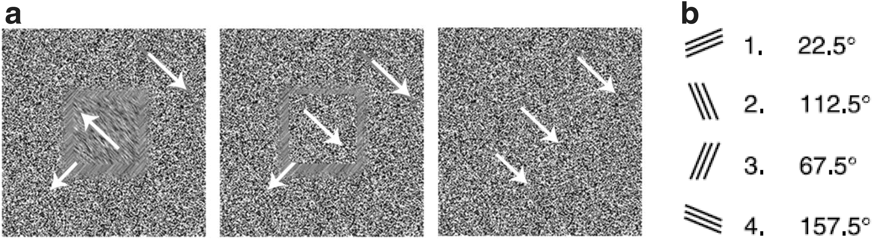
The first part (a) represents the Stack, the Frame, and the Homogenous condition, respectively. The second part (b) represents the four different directions of dot displacement.

In the Frame condition, the dots of the frame region moved in a different direction from the background and the region inside the frame. The Stack condition was similar to the Frame condition, except that the dots within the inner region moved in a different direction from the background as well as from the frame. In the Homogenous condition, the dots in the frame and inner region moved homogenously with regard to the background, in which case almost no frame or inner region movement was visible (see Scholte et al., 2008, for more information). Each trial was presented in 300 msec and was followed by an inter-trial interval of 6 sec. To optimize the measured signal, seven stimuli per trial were presented on the screen: three squares on the left, three on the right side of the screen, and one in the middle.

Magnetic resonance imaging

Scans were conducted on a 3T magnetic resonance scanner (Philips Achieva) that was equipped with a 32-channel SENSE head coil. To obtain DTI and fMRI data, three scanning sessions were performed. The first scanning session was used to acquire DTI data, and the last two scanning sessions were used to acquire the fMRI data. Besides the main task, cortical mappers were used.

fMRI acquisition

The experimental setup was an event-related design, meaning that participants were randomly presented as a Stack, Frame, or Homogenous stimulus; while fMRI recordings of the BOLD response were made at regular intervals. The stimuli were presented in a pseudo-random order for 20 times per stimulus type over two runs. One run lasted for approximately 10.6 min and consisted of acquiring 288 volumes (GE-EPI, 200² mm field of view [FOV]; 80² in-plane resolution; 38 slices, 2.5 mm slice thickness; 0.25 mm slice spacing; repetition time [TR], 2200 msec; echo time [TE], 29.93 msec; flip angle [FA], 80°, SENSE factor 2). Furthermore, high-resolution T1-weighted anatomical images (T1; turbo field echo, 160² mm FOV; 256² in-plane resolution; 160 slices, 1 mm slice thickness; TR, 8.159 msec; TE, 3.73 msec; FA, 8°) were obtained from each subject for registration purposes.

fMRI preprocessing and analysis

Preprocessing and statistical analyses of the functional data were performed with FEAT (FMRI Expert Analysis tool) version 5.98, part of FSL [Oxford Center for Functional MRI of the brain (FMRIB) Software Library (www.fmrib.ox.ac.uk/fsl) (Smith et al., 2004)] and Matlab (Mathworks, Inc.). Preprocessing of functional images included head motion correction, slice time correction, brain extraction, spatial smoothing using a Gaussian kernel of Full Width at Half Maximum of 2 mm, and a high-pass cut-off in the temporal domain using a Gaussian kernel with a standard deviation of 100 s. As a final preprocessing step, the functional data were aligned to the T1 image of the subject, and the data of each subject were transformed to MNI152 (Montreal Neurological Institute) using FNIRT nonlinear registration (Andersson et al., 2008).

Both functional and structural analyses were done for a-priori defined ROIs. Selection of the ROIs was based on a large number of studies on object processing and motion perception (e.g., Albright, 1984; Grill-Spector et al., 2001; Malach et al., 1995; Tanaka, 1996; Watson et al., 1993). The six ROIs were V123, IT cortex, MT area of the left and right hemisphere, and LO area of the left and right hemisphere. Region V123 was defined according to the Jülich histological atlas (Amunts et al., 2005), and the IT cortex was defined according to the Harvard–Oxford cortical structural atlas (available at www.cma.mgh.harvard.edu/).

Since the IT cortex has some overlap with the MT and LO areas, the posterior part of the IT was left out of the IT ROI to prevent overlap. Both the Jülich and the Harvard–Oxford atlas are probabilistic, and, therefore, the threshold of a voxel belonging to the V123 or IT ROI was set at a probability of 25%. Since there are large individual differences for the exact location of the MT and LO areas, we used standard functional mappers to localize these brain regions (Watson et al., 1993). The fMRI settings for these functional mapping scans were the same as described earlier. The data from these mappers were analyzed with a general linear model (GLM), including regressors for each condition (see Scholte et al., 2008 for more details).

The functional data were modeled using a GLM at a single subject level using FMRIB's improved linear model with local autocorrelation correction using an AR(1) model (Woolrich et al., 2001). The event onsets of each trial from a specific condition were convolved with a canonical hemodynamic response function (double gamma) to generate the regressors used in the GLM. Results were rendered on Z statistic images thresholded by Z>5.3 with an uncorrected significance threshold of p=0.05. This resulted in the mean parameter estimates (PE) of only the active voxels of each ROI per trial, condition, and subject.

DTI acquisition

In a different session, diffusion-weighted images (TR 6345 msec, TE 76 msec, FA 90°, 120² mm FOV, 224² in-plane resolution, 60 slices, b=1000 msec) were acquired along 32, 48, and 64 collinear directions for obtaining detailed DW images. Each series of directions was preceded by acquisition of a non-diffusion-weighted volume for purposes of registration and motion correction. The sum of diffusion-weighted volumes was 575 (4*32, 3*48, 2*64). Total acquisition time was 110 min.

DTI preprocessing and analysis

All DTI preprocessing and analyses were conducted using FSL tools (www.fmrib.ox.ac.uk/fsl). Diffusion data were corrected for eddy currents and possible head motion (Jenkinson and Smith, 2001). Next, all non-brain data were discarded, and images were aligned to MNI152 standard space. This ensured that the DTI data were in the same space as the functional data. Images from all subjects were visually inspected to confirm a close registration.

To study the structural connectivity between the six ROIs (V123, IT, MTleft, MTright, LOleft, and LOright; see also fMRI section preprocessing and analysis), we used probabilistic fiber tracking by applying the FMRIB Diffusion Toolkit. Subsequently, the BEDPOSTX tool, which runs a Markov Chain Monte–Carlo estimation process, was used to create distributions of diffusion parameters describing the principle water diffusion direction in each voxel (Behrens et al., 2003). For each voxel included in the ROI or seed mask, 5000 streamline samples were taken from the distribution. This resulted in a probabilistic map indicating the connections of each voxel included in the seed mask with the rest of the brain. Next, the probability map was filtered so that only the streamlines connecting the voxels of two different ROIs, the seed ROI and the target ROI, were taken into account. Probabilistic tractography between two ROIs was done in both directions; for example, from V123 to IT and back. We summed up the number of streamlines that left the seed ROI and reached the target ROI. The number of completed streamlines reflects the confidence that a connection exists at a structural level (Tournier et al., 2011; see also Jones, 2010 for a critical review on DTI as a measure of structural connectivity). These derived pathway strengths are then an (indirect) measure of structural connectivity (Jbabdi and Johansen-Berg, 2011). This number was divided by the volume of the seed and target mask to normalize for between-subject variability in area size.

SEM and AG connectivity analysis

Figure 2 demonstrates the procedure for SEM and AG connectivity analysis. The first three steps are identical for the SEM and AG methods. As described earlier, the event-related BOLD fMRI data were used as input to a GLM, which resulted in PEs of neural activation for all six ROIs (averaged over voxels within ROIs) per condition specific trial. Error trials were excluded from the connectivity analysis. Importantly, connectivity analysis in both SEM and AG is based on the replication of the condition-specific trials and not on the time series. In this way, SEM and AG do not depend on the low temporal resolution of time series in fMRI but on the number of replications per condition (Waldorp et al., 2011). Based on the PEs of single trial data, the covariance matrices for each condition and each subject were determined. Since there were three task conditions and five subjects, this resulted in 15 data covariance matrices.

FIG. 2.

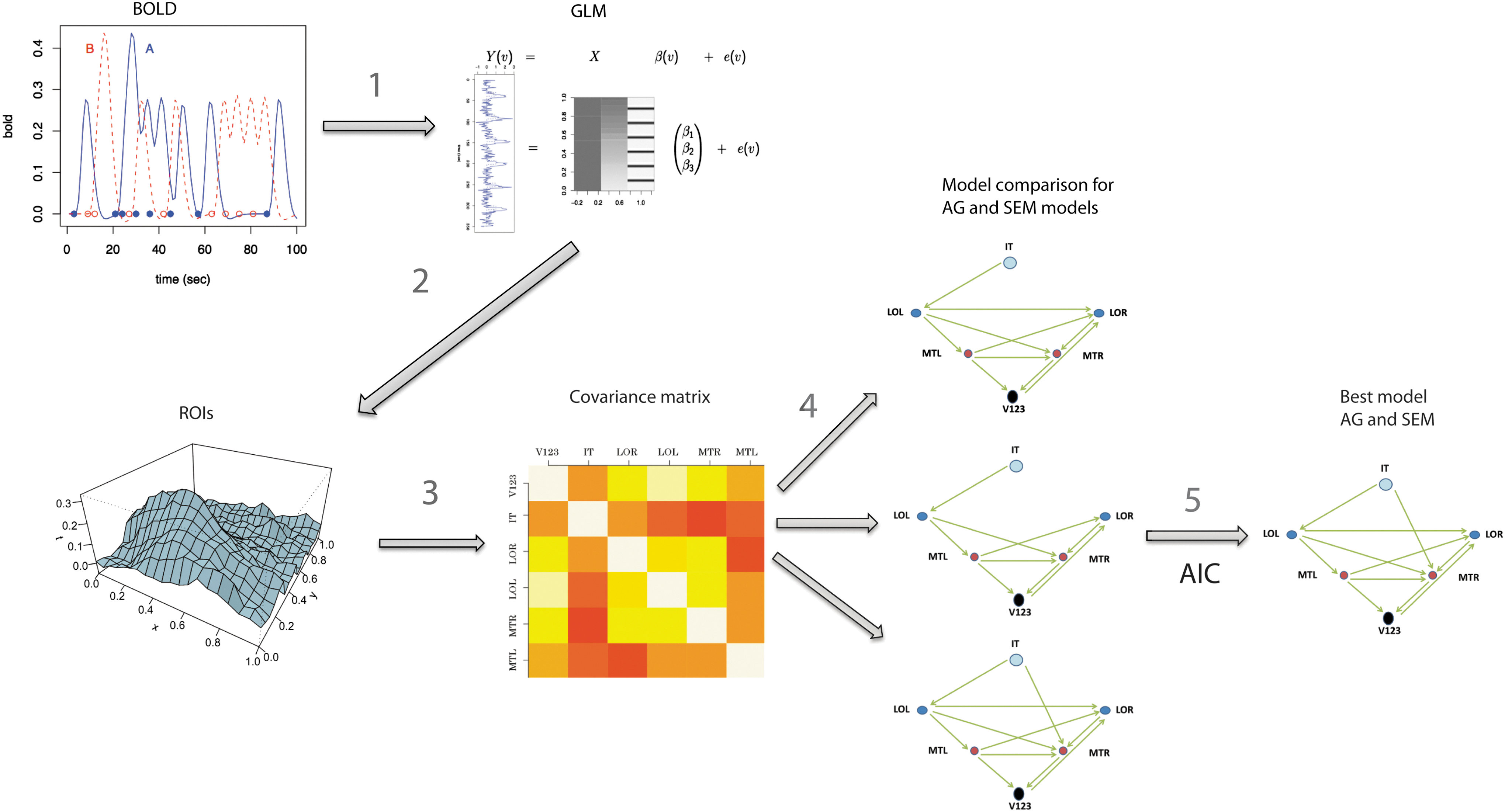
Procedure of effective connectivity analysis for AG and SEM. (1) The event-related BOLD fMRI data are used as input to the GLM. (2) This results in the mean parameter estimates of the neural activation of all six ROIs per condition-specific trial. (3) Based on this, the data covariance matrices for each condition and each subject are determined. (4) Based on the covariance matrices, the model fit of different models is compared. (5) The lower the AIC, the better the model fit. Choosing the best model is based on a joint probability of AIC and robustness probability. AG, ancestral graphs; SEM, structural equation model; fMRI, functional magnetic resonance imaging; BOLD, blood oxygen level dependent; GLM, general linear model; AIC, Akaike's information criterion.

In SEM as well as AG, the parameters of the connectivity models, including the path coefficients or path strengths and the error terms, are estimated by minimizing the difference between the observed and estimated covariance matrix using maximum likelihood. The methods differ, however, in the way in which the population error covariance matrix is modeled. While SEM assumes (most often) that the errors of the regressions (effective connectivity) are uncorrelated, AG distinguishes between correlated and uncorrelated errors (Richardson and Spirtes, 2002), providing a way to determine whether there are missing regions. Consequently, in standard SEM, Σ can only be estimated based on directed connections, regressions, which implies effective connectivity and is indicated by B in SEM (McIntosh and Gonzalez-Lima, 1994). Furthermore, the error structure, denoted by Φ_ɛ , is almost always specified as a diagonal covariance matrix, meaning that the estimated error structure in the model is uncorrelated (Gates et al., 2010; McIntosh and Gonzalez-Lima, 1994).

In AG, two other connection types can be identified besides directed connections (denoted by B): undirected connections (denoted by Λ) and bidirected connections (denoted by Ω). Directed connections are ordinary regression parameters, implying effective connectivity; while undirected connections are partial covariances (unscaled partial correlations), implying functional connectivity. Bidirected connections refer to the covariance of the residuals from the regressions. Such a covariance implies that there is an unexplained structure in the residuals, meaning that a parameter (a brain region) is missing from the model (Waldorp et al., 2011). It should be noted that bidirected connections in AG are not the same as reciprocal connections in SEM; in AG, undirected edges are used to indicate reciprocal information flow and are, therefore, similar to the reciprocal connections in SEM. The covariance matrix is modeled by SEM and AG, respectively: \documentclass{aastex}\usepackage{amsbsy}\usepackage{amsfonts}\usepackage{amssymb}\usepackage{bm}\usepackage{mathrsfs}\usepackage{pifont}\usepackage{stmaryrd}\usepackage{textcomp}\usepackage{portland, xspace}\usepackage{amsmath, amsxtra}\pagestyle{empty}\DeclareMathSizes{10}{9}{7}{6}\begin{document} \begin{align*}{ \rm SEM} : \Sigma = ( I - B ) ^{ - 1} \ \Phi_{\varepsilon} ( I - B^t ) ^{ - 1} \tag{1}\end{align*} \end{document} \documentclass{aastex}\usepackage{amsbsy}\usepackage{amsfonts}\usepackage{amssymb}\usepackage{bm}\usepackage{mathrsfs}\usepackage{pifont}\usepackage{stmaryrd}\usepackage{textcomp}\usepackage{portland, xspace}\usepackage{amsmath, amsxtra}\pagestyle{empty}\DeclareMathSizes{10}{9}{7}{6}\begin{document} \begin{align*}{ \rm AG} : \Sigma = ( I - B ) ^{ - 1} { \Lambda^{ - 1} \ 0 \choose 0 \ \ \ \Omega} ( I - B^t ) ^{ - 1} \tag{2}\end{align*} \end{document}

where I is the identity matrix, t indicates transposition, and −1 indicates inversion. Thus, the AG method can model both effective (directed connections) and functional connectivity (undirected connections), and it can indicate missing regions (bidirected connections) (see Waldorp et al., 2011 for more details); whereas standard SEM only models direct effective connections. How well the estimated covariance matrix of the model fits the data covariance matrix is indicated by Akaike's information criterion (AIC) (Akaike, 1973), which involves the log-likelihood L(θ) with q parameters collected in the vector θ for model or graph G_q : \documentclass{aastex}\usepackage{amsbsy}\usepackage{amsfonts}\usepackage{amssymb}\usepackage{bm}\usepackage{mathrsfs}\usepackage{pifont}\usepackage{stmaryrd}\usepackage{textcomp}\usepackage{portland, xspace}\usepackage{amsmath, amsxtra}\pagestyle{empty}\DeclareMathSizes{10}{9}{7}{6}\begin{document} \begin{align*}AIC ( G_q ) = - 2L ( \theta ) + 2q. \tag{3}\end{align*} \end{document}

The lower the AIC, the better the model fit.

The differences between the AICs of different models are often small, which makes it difficult to distinguish between models. To overcome this problem, we used Akaike weights, that is, we normalized the AIC differences and treated them as probabilities (Burnham and Anderson, 2004; Wagenmakers and Farrel, 2004). This was done with the following formula, where W stands for Akaike weights, Δ is the difference between the lowest AIC and a current model in AICi, exp() is the natural exponent, and R is the number of models in the probability space: \documentclass{aastex}\usepackage{amsbsy}\usepackage{amsfonts}\usepackage{amssymb}\usepackage{bm}\usepackage{mathrsfs}\usepackage{pifont}\usepackage{stmaryrd}\usepackage{textcomp}\usepackage{portland, xspace}\usepackage{amsmath, amsxtra}\pagestyle{empty}\DeclareMathSizes{10}{9}{7}{6}\begin{document} \begin{align*}W_i = \frac { \exp \ ( - \Delta_i / 2 ) } { \Sigma_ { r = 1 } ^R \ \exp ( - \Delta_r / 2 ) } . \tag { 4 } \end{align*} \end{document}

The probabilities were given for the 20 models (R=20) having the lowest AIC. In order to choose the best model of the 20 models selected with the AIC, we also considered the robustness of the model. The degree of robustness depends on how many connections in the model are also present in the other models. A model has a higher degree of robustness if the connections of the model are in all or most of the other 20 models as well, indicating that the connection is invariant over different configurations in a graph. Thus, besides Akaike weights, we also take robustness into account when selecting the best-fitting model. This leads to the following joint probability of AIC and robustness probability: \documentclass{aastex}\usepackage{amsbsy}\usepackage{amsfonts}\usepackage{amssymb}\usepackage{bm}\usepackage{mathrsfs}\usepackage{pifont}\usepackage{stmaryrd}\usepackage{textcomp}\usepackage{portland, xspace}\usepackage{amsmath, amsxtra}\pagestyle{empty}\DeclareMathSizes{10}{9}{7}{6}\begin{document} \begin{align*}& P {(\rm AIC \ and \ robustness\ \mid\ data ) } = P {( \rm AIC\ \mid \ data)} \\ & \quad P {( \rm robustness \mid \ data )} \tag{5}\end{align*} \end{document}

The model with the highest joint probability was selected as the best-fitting model for each subject and condition.

In SEM, composing a model is always hypothesis driven, because no data-driven method is available. We, therefore, constructed models for the SEM method based on previous research. The areas that make up the visual cortex are vastly interconnected. One approach to modeling their organization is to presume that processing is both distributed and hierarchical (Felleman and VanEssen, 1991). From this perspective, it would be expected that information is relayed from the earliest, very broadly tuned, visual areas (V123) to somewhat higher-tier processing stations devoted to motion signals (MT) and object shape perception (LO) before being finally relayed to pure object processing areas (IT). It is, however, clear that there are many projections between different visual areas (Felleman and VanEssen, 1991) and that these, furthermore, not only project from lower-tier to higher-tier areas but also vice versa (Lamme and Roelfsema, 2000).

Based on this, we constructed three models having directed connections that either start from the V123 area going up to the IT area via the MT and LO areas (model 1, see also Fig. 8) or start from the IT area going down to the V123 via LO and/or MT areas (models 2 and 3). These hypothesis-driven models were tested for the different conditions (Homogenous, Frame and Stack condition) with SEM (Mplus version 6.11) (Muthén and Muthén, 2010), and for each condition, the model with the highest joint probability was selected as the best-fitting model.

Since there are many projections between different visual areas, it is difficult to predict how exactly the information flows between the visual areas. Thus, in this case, a more explorative or data-driven method is likely to be beneficial. Furthermore, a data-driven method can lead to new insights on possible connections or directions between the ROIs. Even though there is no data-driven method for SEM, such a data-driven search process has been developed for the AG method in the language R (R Development Core Team, 2011). To make the comparison between AG and SEM more optimal, we used the models found with (data-driven) AG to be fitted with SEM. This resulted in hypothesis-driven SEM models, data-driven SEM models, and data-driven AG models. AG was compared with both hypothesis-driven and data-driven SEM models. Next, we describe the data-driven search process in greater detail.

Since the number of possible models in the AG method is between 14 million and 1.07 billion, it is impossible to test all models. Instead, we developed a method that can find the best-fitting model without testing all models. In this data-driven approach, we started for each of the three conditions with the six ROIs without any connections. Next, a single directed connection entered the model. The fit of this connection was determined for all pairs of ROIs. The connection having the lowest AIC remained in the model. Subsequent connections are obtained in a similar manner. This procedure continued until adding a new connection did not lead to a lower AIC. The same procedure was executed for a combination of directed, undirected, and bidirected connections. For SEM, the best three models that were found with the data-driven AG procedure and contained only directed edges were fitted (Mplus version 6.11) (Muthén and Muthén, 2010). Again, for each condition, the model with the highest joint probability was selected as the best-fitting model. This resulted in 15 models for the AG method and 15 models for the hypothesis- and data-driven SEM method (3 conditions×5 subjects).

Combining effective and structural connectivity

In order to analyze the performance of both AG and SEM with regard to predicting structural connectivity, the connection strengths of the effective connectivity analyses were correlated with the connection probabilities resulting from probabilistic tractography (probtackx in FSL), which reflect the confidence that a connection exists between brain areas. We tested differences between the different methods: AG, SEM (data-driven SEM or SEM supplemented by AG), and SEMS (standard or hypothesis-driven SEM) using normalized scores. Normalization ensured that different scales of each method were not causing differences.

Scores for each method were normalized per subject and per condition (Euclidean distance) across the 30 connections. We used a Wald-type test for the difference between two parameter vectors of connections, which incorporates the covariance matrix of the connections, such as Hotelling's test for MANOVA. Under the null hypothesis of no difference between the vectors of connections, this test has a chi-square distribution (since the parameters of the connections are approximately normally distributed).

The covariance matrix was obtained by assuming that it is the same for all subjects and conditions, such that the data from the different subjects and conditions could be pooled. Then, a lasso estimate of the covariance matrix was obtained using the glasso function in R (Friedman et al., 2008). The degrees of freedom were determined using the Satterthwaite approximation, as is common in linear mixed models. We tested at a Bonferroni corrected level of 0.05/15=0.0033.

Results

Structural connectivity

To study structural connectivity, probabilistic tractography was performed for six ROIs. Figure 3 displays the positions of the ROIs of one subject projected on the MNI 152 brain, whereas ROIs V123 and IT were defined with a probabilistic atlas; ROIs MTleft, MTright, LOleft, and LOright were defined with functional mappers (as described in section “fMRI preprocessing and analysis”). In line with previous research, MT was defined as the activation cluster in IT sulcus, and lateral occipital sulcus and the LO area was defined as the activation cluster between area MT and V123 (Scholte et al., 2008).

FIG. 3.

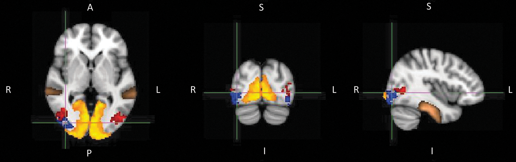
The six ROI. The yellow region is V123, the brown region is IT cortex, the red regions are the temporal motion areas, MTleft and the MTright, and the blue regions are the lateral occipital areas, LOleft and LOright. S, superior; I, inferior; R, right; L, left; A, anterior; ROI, regions of interest; MT, middle temporal; IT, inferior temporal.

The pathway strength between two ROIs was derived from the number of completed paths between two ROIs. In Fig. 4, an example of probabilistic tractography is presented. Tracking starts in this example from ROI MTleft. The two target ROIs presented in the figure are MTright and the LOleft. As the figure shows, almost no tracts from the MTleft area reach the MTright area, whereas a large number of tracts from the MTleft area reach the LOleft area.

FIG. 4.

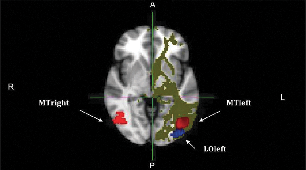
An example of probabilistic tractography as displayed in standard MNI space. The red areas indicate the MT) areas, and the blue area indicates the LO area. Tracking starts in this example from ROI MTleft. The figure shows that more tracts are going from MTleft to LOleft than to MTright. P, posterior; R, right; L, left; A, anterior.

In line with previous findings (Honey et al., 2009; Kaiser and Hilgetag, 2004), connectivity between ROIs decreases with distance between ROIs (Fig. 5). For example, the connection probability between LOleft and V123 is smaller than the connection probability between LOleft and MTleft. Thus, it is less likely that there is a direct structural connection between LOleft and V123 than between LOleft and MTleft.

FIG. 5.

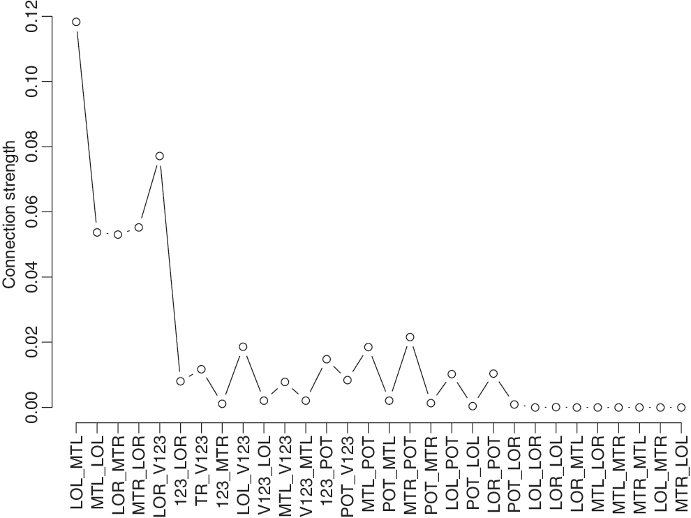
Connection probabilities of DTI connectivity analysis as a function of pairs of ROIs with increasing (Euclidean) distance between ROIs from left to right. Connection probabilities are averaged over all subjects. LL, LOleft; ML, MTleft; LR, LOright; MR, MTright; V, V123. DTI, diffusion tensor images.

Effective connectivity

Effective connectivity analysis using either SEM or AG is based on the replication of the condition-specific trials of the motion perception task (see Figs. 6 and 7). The motion perception task comprised three conditions (Homogenous, Frame and Stack), each consisting of 40 trials. On average, subjects responded correctly to 92.0% of the trials in the Homogenous condition (36.8 trials with a standard deviation (SD) of 2.59), to 86.5% in the Frame condition (34.6 trials with an SD of 5), and to 76.0% in the Stack condition (30.4 trials with an SD of 8.23).

FIG. 6.

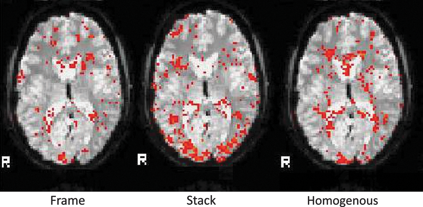
The fMRI data of one trial per condition for one subject. For each condition, the 20th trial of the first run is shown. The fMRI images are images of correctly performed trials. R, right.

FIG. 7.

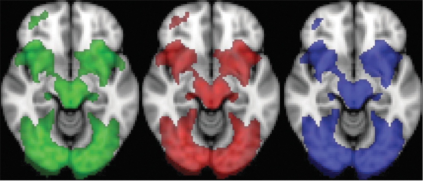
From left to right, the figure shows the activation pattern of, respectively, the Homogenous, Frame, and Stack condition over all runs (within a subject fixed, over subjects mixed).

For each subject and each condition, the best model was selected for the SEM and AG method. Here, the best is defined in terms of Akaike weights and robustness (see Methods). The best three models obtained with the data-driven AG procedure were tested with SEM. Therefore, there are 15 models (5 subjects×3 conditions) for the hypothesis-driven SEM method, the data-driven SEM method, and the data-driven AG method.

An example of the best model for the AG and the data-driven and hypothesis-driven SEM models for the first subject of the Homogenous condition is displayed in Fig. 8. In this particular case, the AG model includes both bidirected connections (displayed in dashed orange arrows) and directed connections (displayed in green solid arrows), whereas the SEM model includes only directed connections. The bidirected connections have a strength of zero, indicating that there is a missing region causing a correlation but no direct connection between the two ROIs.

FIG. 8.

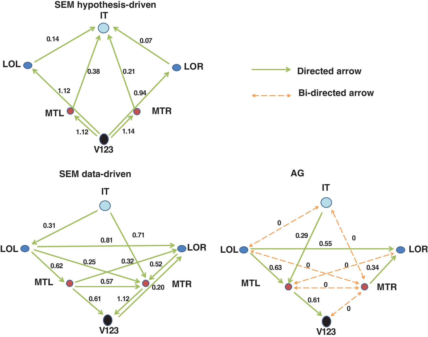
The best-fitting models for the first subject in the Homogenous condition. Orange dotted connections are bidirected connections and indicate that there is a missing region. Green solid connections are directed connections. Besides the connections themselves, the unstandardized strengths of the connections are also presented in the figure.

Validating the AG method using SEM and DTI

To examine whether the AG method can predict structural connectivity equally well or even better than the conventional SEM method, the standardized connection strengths of both the AG and SEM models were correlated with the standardized connection probabilities from tractography (see Fig. 9). Standardization was performed for each subject and condition separately (compare the method of Urbach and Kutas, 2002). The standardized connection strengths have a scale from 0 to 1.

FIG. 9.

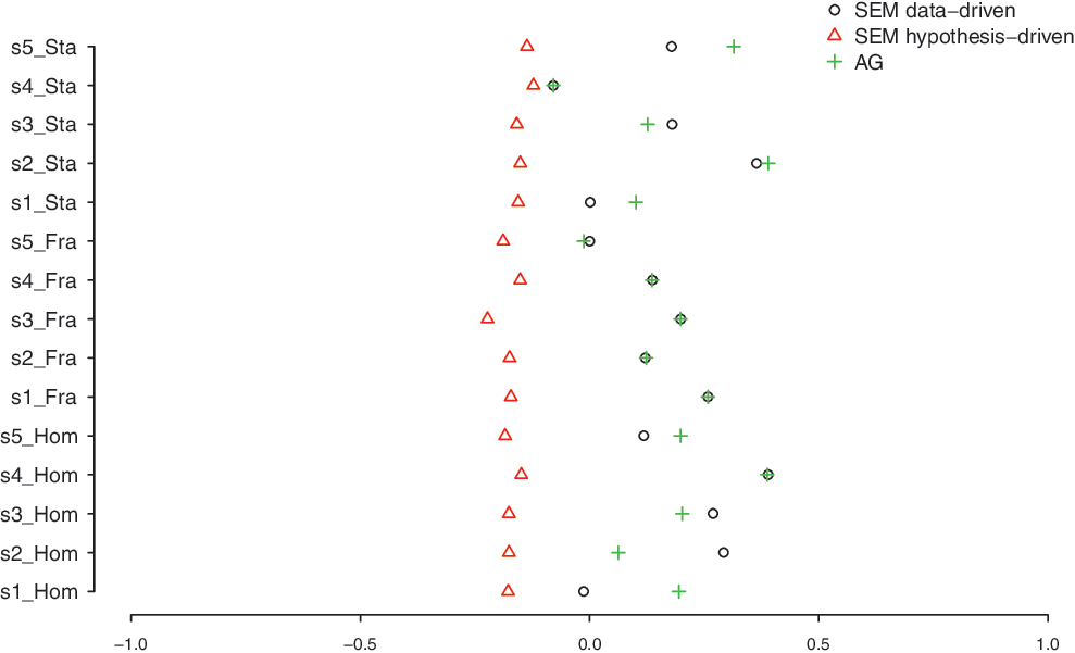
Correlations of AG, SEM, and SEMS methods with DTI values. s, subject; Hom, homogenous condition; Fra, frame condition; Sta, stack condition; SEMS, SEM standard (hypothesis driven).

We tested differences between the different methods: AG, SEM, and SEMS (hypothsis driven) with the normalized scores using a Wald type that has a chi-square distribution under the null hypothesis of no difference. We tested individual and condition-specific tests at 0.05 and subsequent tests for each individual and condition separately (15 in total) at a Bonferroni-corrected level of 0.05/15=0.0033. Overall tests revealed that there were no differences between AG and SEM (χ² [10.71]=8.56, p=0.6382). However, the difference between AG and SEMS was significant (χ² [16.60]=28.99, p=0.0300), and also the difference between SEM and SEMS was significant (χ² [17.09]=29.87, p=0.0282). This indicates that AG and SEM perform equally well, but SEMS performs worse. The results for the individual and condition-specific tests are in Table 1.

Table 1.

Significance Tests of Differences Between Methods of Analysis for 30 Connections

	AG-SEM		AG-SEMS		SEM-SEMS
	df=10.71		df=16.60		df=17.09
Subj-cond	χ²	P	χ²	p	χ²	p
S1-hom	35.04	0.0002^a	53.40	0.0000^a	57.69	0.0000^a
S1-frame	0.00	1.0000	26.23	0.0620	26.24	0.0721
S1-stack	35.87	0.0001^a	36.84	0.0029^a	37.47	0.0030^a
S2-hom	13.58	0.2378	40.57	0.0009^a	41.55	0.0008^a
S2-frame	0.00	1.0000	28.60	0.0334	28.66	0.0389
S2-stack	6.01	0.8573	30.01	0.0226	36.44	0.0042
S3-hom	13.61	0.2361	17.25	0.4099	21.66	0.2022
S3-frame	0.00	1.0000	17.00	0.4266	17.00	0.4602
S3-stack	5.52	0.8910	28.99	0.0300	28.05	0.0457
S4-hom	0.00	1.0000	29.06	0.0295	29.06	0.0350
S4-frame	0.01	1.0000	21.90	0.1709	21.73	0.1995
S4-stack	0.00	1.0000	31.51	0.0148	31.56	0.0176
S5-hom	0.84	1.0000	23.74	0.1134	23.81	0.1276
S5-frame	9.84	0.5187	26.42	0.0590	23.08	0.1500
S5-stack	8.03	0.6872	23.30	0.1255	24.02	0.1217

The degrees of freedom (df) were computed for each method separately using the Satterthwaite approximation.

p-Values are significant at level 0.05/15=0.0033.

AG, ancestral graph; SEM, structural equation modeling (data driven through AG); SEMS, SEM standard (hypothesis-driven).

Most important are the differences between SEM and AG for subject 1 in the homogeneous and stack condition. For this subject in the AG model, six bidirected edges were obtained, indicating no direct connection. This corresponded well with the DTI values. SEM and SEMS, on the other hand, had nonzero coefficients for these connections, making its relation with DTI poor (see also Fig. 8). In the stack condition, the AG model obtained five undirected connections, indicating mutual influence (or at least no direction could be estimated reliably). This also corresponded well with DTI, but not with SEM or SEMS. These results are in line with the results from the correlations.

Discussion

In this study, we examined AGs for studying effective connectivity. AG was compared with the conventional SEM. We compared the more explorative or data-driven AG method with both the standard hypothesis-driven and a data-driven SEM method. For the data-driven SEM method, we used the models found with AG, as no data-driven method is currently at hand for SEM. We used the data-driven AG and SEM and the hypothesis driven-SEM methods to estimate the connection strength between six ROIs of the visual cortex based on fMRI data of a motion perception task. The achieved effective connection strengths between the ROIs of all methods were correlated with connection probabilities derived from the DTI analysis to compare the performance between AG and SEM methods.

Results indicated that the least accurate models were the models of the hypothesis-driven SEM method. The hypothesis-driven SEM method performed worse than both the data-driven SEM and the AG method. This is probably due to the complicated structure of projections between different visual areas (Felleman and VanEssen, 1991), going not only from lower-tier to higher-tier areas but also vice versa (Lamme and Roelfsema, 2000). At this moment, too little is known about this exact information flow between the different regions, which makes it logical that an explorative model has a better fit than a theory-based model.

A comparison of the data-driven SEM and AG methods showed that, in general, the AG and the SEM method predicted structural connectivity equally well. We performed the correlational analyses for each subject and condition separately. Only in the Homogenous and Stack condition of the first subject, the AG method predicted structural connectivity significantly better than the SEM method. In the Homogenous condition and the Stack condition of this subject, the AG models contained a lot of bidirected or undirected connections, respectively. This seems to indicate that whenever there are possibly missing regions, as indicated by the bidirected connections, the AG method outperforms SEM.

Furthermore, it is beneficial for SEM to use models that are based on a selection from AG. Using AG to compose models for SEM has led to models that usually would not be found with SEM. Thus, AG can lead to more informative and accurate models of brain networks in future connectivity research.

Conclusion

This study showed that AG is a fruitful method to study effective connectivity. In contrast to conventional methods to study effective connectivity, such as SEM, AG can detect, besides directed connections, whether there are undirected connections, indicating mutual influence (or at least no direction could be estimated reliably) and bidirected connections, indicating that there is a missing region causing a correlation but no direct connection between the two ROIs. In particular, the ability to detect missing regions is a unique feature of AG that leads to network models with fewer spurious connections.

Footnotes

Acknowledgments

The authors would like to thank Martijn Wokke for helping setting up the experiment and the subjects who participated in the experiment. Furthermore, they would like to thank Markus Eronen and the two anonymous referees of this journal for their helpful comments.

Authors Disclosure Statement

The authors have no competing financial interests.

References

Akaike

. 1973. Information and an extension of the maximum likelihood principle. Petrov

, Csáki

. Proceedings of the Second International Symposium on Information Theory. Budapest: Akademia Kiado, 267–281.

Albright

. 1984. Direction and orientation selectivity of neurons in visual area MT of the macaque. J Neurophysiol, 52:1106–1130.

Albright

, Stoner

. 1995. Visual motion perception. Proc Natl Acad Sci U S A, 92:2433–2440.

Amunts

, Kedo

, Kindler

, Pieperhoff

, Mohlberg

, Shah

, Habel

et al. 2005. Cytoarchitectonic mapping of the human amygdala, hippocampal region and entorhinal cortex: intersubject variability and probability maps. Anat Embryol, 210:343–352.

Andersson

, Smith

, Jenkinson

. 2008. FNIRT—FMRIB's non-linear image registration tool. Poster presented at the annual meeting of the Organization Human Brain Mapping, Melbourne, Australia.

Behrens

TEJ

, Woolrich

, Jenkinson

, Johansen-Berg

, Nunes

, Clare

, Matthews

, Brady

, Smith

. 2003. Characterization and propagation of uncertainty in diffusion-weighted MR imaging. Magn Reson Med, 50:1077–1088.

Büchel

, Friston

. 1997. Modulation of connectivity in visual pathways by attention: cortical interactions evaluated with structural equation modeling and fMRI. Cereb Cortex, 7:768–778.

Bullmore

, Sporns

. 2009. Complex brain networks: graph theoretical analysis of structural and functional systems. Nat Rev Neurosci, 10:186–198.

Burnham

, Anderson

. 2004. Multimodel inference: understanding AIC and BIC in model selection. Soc Methods Res, 33:261–304.

10.

Eichler

. 2005. A graphical approach for evaluating effective connectivity in neural systems. Philos Transact R Soc B, 360:953–967.

11.

Felleman

, VanEssen

. 1991. Distributed hierarchical processing in the primate cerebral cortex. Cereb Cortex, 1:1–47.

12.

Friedman

, Hastie

, Tibshirani

. 2008. Glasso: graphical lasso- estimation of Gaussian graphical models. R package version 1.4. http://cran.r-project.org/web/packages/glasso/index.html

13.

Friston

. 2011. Functional and effective connectivity: a review. Brain Connect, 1:13–36.

14.

Friston

, Harrison

, Penny

. 2003. Dynamic causal modelling. Neuroimage, 19:1273–1302.

15.

Gates

, Molenaar

, Hillary

, Ram

, Rovine

. 2010. Automatic search for fMRI connectivity mapping: an alternative to Granger causality testing using formal equivalences among SEM path modeling, VAR, and unified SEM. Neuroimage, 50:1118–1125.

16.

Gonçalves

, Hall

. 2003. Connectivity analysis with structural equation modeling: an example of the effects of voxel selection. Neuroimage, 20:1455–1467.

17.

Grill-Spector

, Kourtzi

, Kanwisher

. 2001. The lateral occipital complex and its role in object recognition. Vis Res, 41:1409–1422.

18.

Guye

, Bartolomei

, Ranjeva

. 2008. Imaging structural and functional connectivity: towards a unified definition of human brain organization? Curr Opin Neurol, 24:393–403.

19.

, Evans

. 2010. Graph theoretical modeling of brain connectivity. Curr Opin Neurol, 23:341–350.

20.

Honey

, Sporns

, Cammoun

, Gigandet

, Thiran

, Meuli

, Hagmann

. 2009. Predicting human resting state functional connectivity from structural connectivity. Proc Natl Acad Sci U S A, 106:2035–2040.

21.

Horwitz

, Warner

, Fitzer

, Tagamets

, Husain

, Long

. 2005. Investigating the neural basis for functional and effective connectivity. Application to fMRI. Philos Trans R Soc Lond B Biol Sci, 360:1093–1108.

22.

Jbabdi

, Johansen-Berg

. 2011. Tractography: where do we go from here? Brain Connect, 1:169–183.

23.

Jenkinson

, Smith

. 2001. Global optimisation method for robust affine registration of brain images. Med Image Anal, 5:143–156.

24.

Johansen-Berg

, Behrens

. 2006. Just pretty pictures? What diffusion tractography can add in clinical neuroscience. Curr Opin Neurol, 19:379–385.

25.

Jones

. 2010. Challenges and limitations of quantifying brain connectivity in vivo with diffusion MRI. Imaging Med, 2:341–355.

26.

Kaiser

, Hilgetag

. 2004. Modelling the development of cortical systems networks. Neurocomputing, 58:297–302.

27.

Lamme

VAF

, Roelfsema

. 2000. The distinct modes of vision offered by feedforward and recurrent processing. Trends Neurosci, 23:571–579.

28.

Malach

, Reppas

, Benson

, Kwong

, Jiang

, Kennedy

, Ledden

, Brady

, Rosen

, Tootell

RBH

. 1995. Object-related activity revealed by functional magnetic resonance imaging in human occipital cortex. Proc Natl Acad Sci U S A, 92:8135–8138.

29.

McIntosh

, Gonzalez-Lima

. 1994. Structural equation modeling and its application to network analysis in functional brain imaging. Hum Brain Mapp, 2:2–22.

30.

McIntosh

, Grady

, Haxby

, Ungerleider

, Horwitz

. 1996. Changes in limbic and prefrontal functional interactions in a working memory task. Cereb Cortex, 6:571–584.

31.

Muthén

, Muthén

. 2010. Mplus User's Guide. 6th. Los Angeles, CA: Muthén & Muthén.

32.

Oldfield

. 1971. The assessment and analysis of handedness: the Edinburgh inventory. Neuropsychologia, 9:97–114.

33.

Penny

, Stephan

, Mechelli

, Friston

. 2004. Comparing dynamic causal models. Neuroimage, 22:1157–1172.

34.

R Development Core Team. 2011. R: a language and environment for statistical computing. Vienna, Austria: R Foundation for Statistical Computing www.R-project.org/. 2012 Nov. 9.

35.

Ramsey

, Hanson

, Halchenko

, Poldrack

, Glymour

. 2010. Six problems for causal inference from fMRI. Neuroimage, 49:1545–1558.

36.

Richardson

, Spirtes

. 2002. Ancestral graph markov models. Annual Statist, 30:962–1030.

37.

Roebroeck

, Formisano

, Goebel

. 2005. Mapping directed influence over the brain using granger causality and fmri. Neuroimage, 25:230–242.

38.

Rubinov

, Sporns

. 2010. Complex network measures of brain connectivity: Uses and interpretations. Neuroimage, 52:1059–1069.

39.

Rykhlevskaia

, Gratton

, Fabiani

. 2008. Combining structural and functional neuroimaging data for studying brain connectivity: a review. Psychophysiology, 451:73–87.

40.

Scholte

, Jolij

, Fahrenfort

, Lamme

VAF

. 2008. Feedforward and recurrent processing in scene segmentation: electroencephalography and functional magnetic resonance imaging. J Cogn Neurosci, 20:2097–2107.

41.

Smith

, Jenkinson

, Woolrich

, Beckmann

, Behrens

, Johansen-Berg

, Bannister

, De Luca

, Drobnjak

, Flitney

, Niazy

, Saunders

, Vickers

, Zhang

, De Stefano

, Brady

, Matthews

. 2004. Advances in functional and structural MR image analysis and implementation as FSL. Neuroimage, 23:208–219.

42.

Tanaka

1996. Inferotemporal cortex and object vision. Annu Rev Neurosci, 19:109–139.

43.

Telesford

, Simpson

, Burdette

, Hayasaka

, Laurienti

. 2011. The brain as a complex system: using network science as a tool for understanding the brain. Brain Connect, 1:295–308.

44.

Tournier

J-D

, Mori

, Leemans

. 2011. Diffusion tensor imaging and beyond. Magn Reson Med, 65:1532–1556.

45.

Urbach

, Kutas

. 2002. The intractability of scaling scalp distributions to infer neuroelectric sources. Psychophysiology, 39:791–808.

46.

Van den Heuvel

, Hulshoff Pol

. 2010. Exploring the brain network: a review on resting-state fMRI functional connectivity. Eur Neuropsychopharmacol, 20:519–534.

47.

Wagenmakers

E-J

, Farrell

. 2004. AIC model selection using Akaike weights. Psychon Bull Rev, 11:192–196.

48.

Waldorp

, Christoffels

, van den Ven

. 2011. Effective connectivity of fMRI data using ancestral graph theory: dealing with missing regions. Neuroimage, 54:2695–2705.

49.

Watson

, Myers

, Frackowiak

, Hajnal

, Woods

, Mazziotta

, Shipp

, Zeki

. 1993. Area V5 of the human brain: evidence from a combined study using positron emission tomography and magnetic resonance imaging. Cereb Cortex, 3:79–94.

50.

Woolrich

, Ripley

, Brady

, Smith

. 2001. Temporal autocorrelation in univariate linear modeling of FMRI data. Neuroimage, 14:1370–1386.

51.

Zhang

, Snyder

, Fox

, Sansbury

, Shimony

, Raichle

. 2008. Intrinsic functional relations between human cerebral cortex and thalamus. J Neurophysiol, 100:1740–1748.