
Abstract
Two aspects play a key role in recently developed strategies for functional magnetic resonance imaging (fMRI) data analysis: first, it is now recognized that the human brain is a complex adaptive system and exhibits the hallmarks of complexity such as emergence of patterns arising out of a multitude of interactions between its many constituents. Second, the field of fMRI has evolved into a data-intensive, big data endeavor with large databases and masses of data being shared around the world. At the same time, ultra-high field MRI scanners are now available producing data at previously unobtainable quality and quantity. Both aspects have led to shifts in the way in which we view fMRI data. Here, we review recent developments in fMRI data analysis methodology that resulted from these shifts in paradigm.
Introduction
“More is different” was the title of a seminal work published in 1972 by the Nobel Prize winner P.W. Anderson (Anderson, 1972). It was one of the first articles to recognize the complexity of large-scale systems and the implications this might have on progress in science. In the field of functional magnetic resonance imaging (fMRI), it is now widely accepted that patterns of activation and their complex interactions distributed across large parts of the brain are fingerprints of cognitive processes, so that the whole is, in fact, larger than the sum of its parts. In this sense, more may really be different. While this insight is taking hold, a second aspect sometimes called “big data” or “data-intensive research” has engulfed fMRI (Bell et al., 2009). Examples of this are the Connectome project (Van Essen et al., 2012), the International Neuroimaging Data-sharing Initiative (Biswal et al., 2010), or the BrainMap database (Laird et al., 2005), each providing access to thousands of datasets. In addition, ultra-high field MRI with its increased spatial resolution and massive data volumes requires data-intensive research, allowing us to address questions that were previously beyond reach (Bandettini et al., 2012).
These new developments have necessitated a paradigm shift in data analysis strategies for fMRI data. Here, we will review recent methodological advances in this field. Our focus will be on the design of algorithms rather than on the neuroscientific results they have produced. “More is different” provides a common ground for both trends that also implies methodological commonalities.
Most (if not all) researchers today will agree that the human brain is a complex adaptive system (e.g., Breakspear and McIntosh, 2011; Bullmore and Sporns, 2009; Koch and Laurent, 1999; Logothetis, 2012; Panagiotaropoulos et al., 2012; Skarda and Freeman, 1990; Sporns, 2011b; Tononi et al., 1994). However, it is often not quite clear what this term actually means, nor what it entails with respect to the analysis strategy used on our fMRI data. There is at present no rigorous and generally accepted definition of the term “complex system” or “complex adaptive system.” The term “complex” is sometimes simply considered to be synonymous with “complicated.” However, a large body of literature now exists that provides a deeper and more interesting picture. So, what is a “complex adaptive system”? John Holland, who is one of the pioneering researchers in the field of complex systems, wrote “CAS (complex adaptive systems) are systems that have a large number of components, often called agents, that interact and adapt or learn.” (Holland, 2006).
One of the key features of complexity is thus the sheer size of the system. Small systems with few constituents can never display a considerable complexity by this definition (see also Baranger, 2012). Geometric studies suggest that this property is more dominant in systems with a large number of constituents (Ay et al., 2011). Systems with many constituents have a higher probability of developing an adaptation process to increase complexity. In this context, scaling properties of various complexity measures have been studied in (Olbrich et al., 2008).
According to Baranger (2012), complexity is quite distinct from chaos. Chaos is characterized by high sensitivity to initial conditions resulting in unpredictable behavior (not to be confused with random noise), while the hallmark of complexity is emerging behavior and a tendency toward self-organization (Rickles et al., 2007). Complex systems exhibit an interplay of chaos and complexity, whereas fully chaotic systems are unpredictable in their entire phase space. Very small systems can be fully chaotic (e.g., a double pendulum), while complexity requires positive feedback mechanisms as well as a large number of nonlinearly interacting agents. If our brains were merely chaotic, but not complex, we would certainly not be able to survive.
Another aspect to be considered is that the complex system inside our brain is not static, but changes over time and is thus termed an adaptive system. We need to distinguish adaptability due to the fast dynamics of activation patterns versus the slower changes in synaptic coupling strength. Both aspects come into play and leave traces in the data that we measure.
Several recent studies show that complexity is apparent even at the macroscopic level measured with fMRI. For instance, Achard and colleagues (2006) showed evidence for properties found in many real-world complex networks, such as small worldness (Song and Makse, 2005). Furthermore, Gonzalez-Castillo and colleagues (2012) showed that even very simple paradigms may produce activations in almost the entire brain, which suggests that a large network may have been activated. The emergence of resting-state spontaneous fluctuations and the spatiotemporal patterns they produce may also be seen as indications of complexity (Biswal et al., 2010). Fraiman and Chialvo (2012) as well as Kitzbichler and colleagues (2009) recently reported evidence of self-organized criticality in fMRI data. For more information, see also Stam and Reijneveld, 2007; Vértes et al., 2012.
The second topic big data is also rapidly gaining importance. A well-known example of data-intensive research is the recent initiative to collect resting-state fMRI data of more than 1400 volunteers at 35 international centers (Biswal et al., 2010). The idea is to map an individual's functional connectome and investigate its variations across genetic influences and brain–behavior relationships. At ultra-high field strengths (≥7 T), the data volume increases drastically with the improved spatial resolution that becomes feasible. While conventional fMRI at (3 mm)3 resolution requires about 50,000 voxels to cover the entire brain, ultra-high field fMRI at (1.5 mm)3 resolution takes about 400,000 voxels to cover the same area. Explorative, machine learning-based strategies are needed to harvest this data treasure and new data analysis methods for this purpose are currently being developed or are already in existence.
Two distinct classes of algorithms are relevant for the topics described above (see Fig. 1). The first class identifies spatial patterns of connectivity in voxel space. It is related to the notion of complex systems in that this class of methods is designed to analyze emergent patterns.
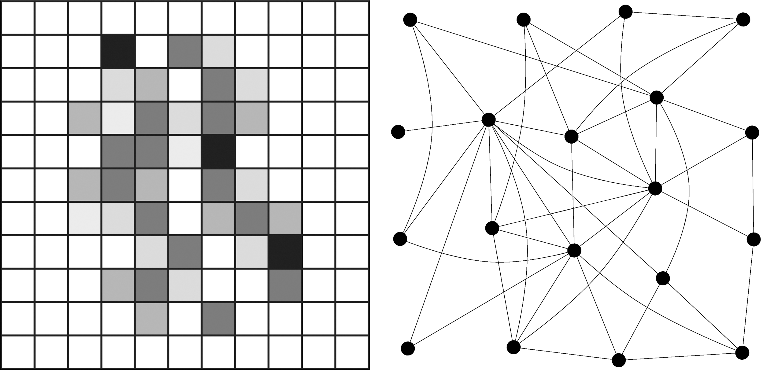
Networks represented by spatial patterns in voxel space (left) versus networks as graphs (right).
Matrix decomposition techniques, such as independent component analysis (ICA), belong to this group as well as machine learning methods such as multivariate pattern classification techniques (multivariate pattern analysis [MVPA]) (Haxby, 2012). MVPA is particularly relevant for the analysis of ultra-high field fMRI data in that it does not require spatial smoothing and can thus make full use of the increased spatial resolution.
The second class of algorithms arise from the new field of network science (Sporns, 2011a). These algorithms are designed to analyze properties of networks that are characteristic of complex systems. They are also highly relevant in the emerging data-intensive (big data) research that is rapidly gaining importance. In this article, we will give an overview of these two classes of algorithms and review their impact on the field.
Spatial Patterns in Voxel Space
In this chapter, we are interested in functional networks that are represented as spatial patterns of connectivity in voxel space. These patterns are characterized by whole brain maps in which each voxel describes the degree of membership in a pattern, where the term “connectivity” refers to correlations between fMRI time series. As discussed in more detail later on, such correlations can be defined by various measures. Patterns may overlap so that a voxel may belong to different patterns to different degrees and membership may change over time. Analysis algorithms in this domain are multivariate and aim to analyze or detect spatial patterns rather than fuzzy blobs.
Preprocessing strategies
Before we begin to review the analysis methods, let us first note that fMRI data need to be preprocessed before any of these techniques can be applied. Various preprocessing strategies have been implemented and recommended. However, the choice of strategy can have a troublingly large impact on the final results. In particular, physiological noise, such as respiration or heart beat, may bias results and is often regressed out (Birn et al., 2008). However, global signal regression as a surrogate for suppressing the effect of physiological noise has been the object of some controversy (Murphy et al., 2009; Weissenbacher et al., 2009).
A comprehensive review of the many preprocessing strategies is beyond the scope of this article. We refer the reader to excellent articles by Strother (2006) and Carp (2012).
Measures of association
Multivariate techniques to be discussed later on in this chapter require the specification of a measure of association between fMRI time courses. In the following, we discuss several such measures that have played prominent roles in this context. For a very careful experimental evaluation of some of these measures based on a simulation study, see also Smith et al., 2011.
Correlation-based measures
Pearson's linear correlation is a bivariate linear measure of association with values ranging between +1 and −1. Linear correlations between fMRI time series are sometimes used synonymously with the term “functional connectivity.” In fact, the majority of seed-based functional connectivity studies are based on linear correlations. The basic strategy is to start with a user-specified seed voxel or region of interest (ROI) and test time courses in the remaining voxels for correlations with the seed. This strategy was successfully used in a number of studies, perhaps one of the most famous example being the study published by Biswal and colleagues (1995). Many other publications too numerous to list have followed since then.
Note that linear correlation can only detect linear dependencies between time series. Therefore, uncorrelatedness is not equivalent to independence because of the potential presence of nonlinear dependencies. Equivalence only holds in the special case when the two time series are jointly normal. Therefore, one should take care to avoid false conclusions about independence when linear correlations were used.
Spearman's rank correlation measures the linear correlation between ranks of values rather than the values themselves. Therefore, this measure is slightly less prone to errors of this type. Partial correlation can be used to measure the degree of linear association between two time series with the effect of other influences regressed out. Smith and colleagues (2011) found that partial correlation gave high sensitivity and performed comparatively well.
Frequency-based measures
As noted by Salvador and colleagues (2005), interregional dependencies can often be more readily observed in the frequency domain than in the time domain. The two most commonly used measures of association in the frequency domain are spectral coherence and wavelet coherence. In both cases, two time courses are considered to be coherent if their power spectra correlate for a given frequency window. Both measures ignore phase shifts, which makes them insensitive to a fixed lag between two time series.
Their main difference is that spectral coherence assumes stationarity of the signals, whereas wavelet coherence does not. Therefore, spectral coherence is insensitive to changes in the coupling between the two time series. It was used for fMRI data analysis in Salvador and colleagues (2005), Müller and colleagues (2003, 2007), and Lohmann and colleagues (2010).
Wavelet coherence was used in fMRI in many studies (e.g., Achard et al., 2006). Chang and Glover (2010) used it to investigate the nonstationary effects of the coupling. Some care must be taken because much of the power in fMRI signals resides in very slow fluctuations around 1/30 Hz. In other words, only about two of these very slow fluctuations occur within 1 min of measurement time. Therefore, to be able to reliably observe effects of nonstationarity, the time series must be long enough to cover several occurrences of these very slow waves.
Granger causality
Perhaps, the best known measure of directed connectivity is Granger causality (GC). A time series X is said to Granger cause some other time series Y if knowledge of past values of X helps to predict future values of Y in a statistically significant way. It is assumed that the data can be adequately described by a linear autoregressive model of some user-specified order p, where p generally ranges between one and four. It was introduced to the fMRI community by Roebroeck and colleagues (2005). For a recent review and recent developments regarding GC, see for example, Deshpande et al., 2010.
The application of GC to fMRI data has been controversial. Smith and colleagues (2011) investigated GC in the context of the simulation study mentioned above. They found that measures based on temporal lags such as GC performed very poorly. Their main point of critique was that the variability of the BOLD response makes the interpretation of temporal effects prone to error. Inter-regional differences in the hemodynamic response function may, in fact, be due to differences in the vasculature rather than to neuronal effects. For an experimental evaluation of the variability of the BOLD response, see e.g., Neumann et al., 2003.
However, rebutting this critique, Schippers and colleagues (2011) claimed that GC fared not so badly when used at the group level, rather than at the individual subject level. They reported that the directional information found by GC was “accurate in the vast majority of the cases.” Smith and colleagues (2012a) responded by noting that there may be a systematic bias not only at the single-subject level, but also at the group level, so that the conclusion drawn by Schippers and colleagues should be taken with care.
This debate was recently taken up by Seth and colleagues (2013). They show that even though GC is surprisingly robust to a wide variety of changes in hemodynamic response properties, it is still prone to error in the presence of heavy measurement noise or severe downsampling. Since both effects are typical of fMRI data, it would be inappropriate to give an all-clear signal for GC.
A possible solution to this problem was proposed by Deshpande and colleagues (2009). They note that a version of GC called “directed transfer function (DTF)” may be appropriate for fMRI data provided it is used in a way that is compatible with the true temporal resolution of the hemodynamic response, namely, at a scale of 6–12 sec. Using a this much reduced temporal resolution, they found that the primary motor area had a causal influence on the supplementary motor area, premotor area, and cerebellum.
Another problem inherent in bivariate directed measures such as pairwise GC is that misleading information may result if the system at hand has interdependencies among more than two nodes (see e.g., Blinowska et al., 2004). In this case, bivariate measures are often inadequate and should be replaced by multivariate methods. Figure 2 shows an example where a trivariate model would be required to disambiguate the two cases.
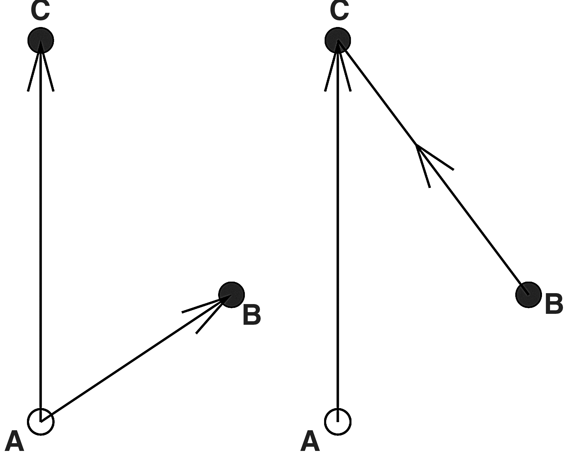
These two cases cannot be disambiguated using bivariate Granger causality.
Note, however, that the number of coefficients to be estimated for a multivariate autoregressive linear model is quadratic in the number of nodes (Harrison et al., 2003). For instance, if the model order p is two and the number of nodes d is five, then the number of coefficients to be estimated is k=p×d×d=50. In the case of fMRI, this may be problematic. The number of data points required for a reliable estimation of a multivariate autoregressive model should be many times larger than k, so that very long time series are needed. In fMRI, time courses generally only contain a few hundred data points so that this requirement may be hard to meet. Nonetheless, Deshpande and colleagues (2011) recently presented a multivariate GC analysis using 33 ROIs, and Tang and colleagues (2012) applied a highly multivariate GC to every voxel within two ROI.
Measures based on information theory
Mutual information
To avoid the limitations of linear correlations, it is sometimes advantageous to assess functional connectivity using mutual information as a measure of higher order statistical dependence. In the context of fMRI analysis, this was, for instance, recently done in a study by Ma and colleagues (2012). Mutual information is a nonlinear measure based on information theory defined as
where p(x, y) is the joint probability distribution function of X and Y, and p(x), p(y) are the marginals. Estimation of density functions can be cumbersome and inaccurate. In the special case, when the two time series are known to be Gaussian with zero mean, unit variance, then a much simpler formula exists (Kraskov et al., 2004). Let cov denote the covariance between X and Y, then
Transfer entropy
Another information theoretic measure of association called Transfer entropy (TE) was introduced by Schreiber (2000). In contrast to mutual information, it allows to describe directed relationships. The idea is to measure the degree to which knowledge of the time course in some voxel j at time n helps to predict the value at some other time course i at time n+1. In other words, we are interested in the deviation from the Markov property p(in
+1|in
, jn
)=p(in
+1|in
). TE is defined as
In the absence of information flow from j to i, knowledge of jn will not help to predict in +1 so that p(in +1|in , jn )=p(in +1|in ) and T=0. A large value of T indicates a strong influence from j to i. TE and multivariate extensions of it were applied to fMRI data in Chai and colleagues (2009), Hinrichs and colleagues (2006), and later also in Lizieri and colleagues (2011).
TE bears some resemblance to GC. The main difference is that GC is a parametric method that requires that the data can be described by a linear autoregressive model. TE on the other hand makes no prior assumptions about the structure of the data and thus allows detection of nonlinear relationships. However, since TE is based on temporal lags in the hemodynamic response, it is plagued by the same problems and controversies that hold for GC.
Matrix decompositions
A prominent class of methods for identifying patterns of connectivity is based on matrix decompositions. Such decompositions are used to factorize the data into weighted components representing these patterns. Mathematically, matrix decompositions can be described as follows. Suppose there are m real-valued data vectors of length n, for instance, fMRI time courses in m voxels measured at n time points arranged in an n×m matrix V. Alternatively, the matrix V may also be an m×m correlation matrix. We then seek approximate factorization of the form:
The spatial patterns to be identified are encoded as rows in the matrix H with weights in the columns of W. In the following, we review several types of matrix factorization that have been used in the context of fMRI data analysis.
Principal component analysis
Principal component analysis (PCA) is a classical approach to matrix factorization. It was originally invented by Pearson (1901). It is used to obtain maximally decorrelated components.
Mathematically, it can be described as follows. Let V be a real-valued p×q matrix whose rows are measurement vectors, for example, fMRI time series. The columns of V must be centered, that is, their means must be subtracted. Let C be the p×p covariance matrix of V, and E the matrix of eigenvectors of C. Since E is orthogonal, EET
equals the identify matrix I, and hence
Let the eigenvectors in E be sorted such that the leftmost columns belong to the largest eigenvalues, and let W denote the matrix consisting of the r leftmost columns of E. Then, an approximation to the matrix V can be obtained by
Thus, with H=WTV, we have a matrix decomposition of the form V≈W H. The first principal components contain most of the variation in the data.
PCA was first applied to fMRI data by Friston and colleagues (1993) who aimed at identifying spatially decorrelated activity patterns. Nowadays, PCA is often used as a data reduction step to be followed by other methods such as ICA.
Independent component analysis
While the aim of PCA is to obtain maximally decorrelated components, ICA is intended to produce maximally independent components (Bell and Sejnowski, 1995). In this sense, ICA can be seen as a special case of blind source separation (BSS). Since very good reviews about ICA exist, we keep this section short and refer the reader to other references (e.g., Calhoun et al., 2009; Kiviniemi et al., 2003; Margulies et al., 2010).
In ICA, we assume that the data can be represented as a mixture of independent sources so that the data matrix V can be approximated as V≈W S, where W is a mixing matrix usually assumed to be square and invertible, and S is a matrix of source signals that we try to recover. The sources can then be reconstructed by inverting the mixing matrix so that the final outcome of an ICA decomposition is
where W −1 is sometimes referred to as the “unmixing matrix.” Many procedures for estimating the unmixing matrix exist (see e.g., Hyvärinen and Oja, 2000).
ICA was introduced into fMRI data analysis by McKeown and colleagues (1998), and later became one of the principal tools for analyzing resting-state fMRI data (Beckmann et al., 2005). In a highly cited study, Smith and colleagues (2009) reported that ICA components at the resting brain match up well with patterns of activations found in the BrainMap database of functional imaging studies (Laird et al., 2005). They concluded that networks in the brain are continuously active even when at rest.
Methodological extensions to the original ICA were, for instance, proposed in Beckmann and Smith (2005), who described a tensorial ICA that allows investigating groups of subjects rather than single-subject data. Most recently, decompositions into the temporal rather than spatial components were discussed in Smith and colleagues (2012b).
Both PCA and ICA require specification of a model order, that is, the number of components to be expected. Since the intrinsic dimensionality of the data is unknown, the selection of an appropriate model order is a difficult problem. For more details, see for example, Abou-Elseoud and colleagues (2010), Li and colleagues (2007), and Yourganov and colleagues (2011).
In addition to the difficulty of specifying model order, the selection and interpretation of meaningful components may often be quite problematic. Furthermore, Daubechies and colleagues (2009) have noted that two ICA algorithms most commonly used for fMRI (InfoMax and FastICA) seem to select for sparsity rather than for independence (Daubechies et al., 2009). In other words, ICA tends to lead to decompositions in which components are sparse in the sense that many of their voxels are close to zero [see Daubechies et al. (2009) for a discussion of the terms “independence/sparsity/separability”]. As a consequence, the authors suggest developing decomposition methods that directly target sparsity instead of independence. In the following paragraph, we introduce an alternative decomposition technique, which may perhaps be useful in this regard.
Non-negative matrix factorization
An alternative to ICA is non-negative matrix factorization (NMF) (Lee and Seung, 1999; Paatero and Tapper, 1994). In contrast to ICA, the components obtained by NMF are not designed to be independent. Rather, the aim is to obtain a decomposition into additive parts. NMF produces a decomposition of the n×m data matrix V such that
with W an n×r
NMF can be seen as a form of BSS with non-negativity constraints. Non-negativity is a sensible requirement as the networks that are detected by decomposition techniques can only be present or absent, but not negatively present. Thus, negative weights for networks are difficult or even impossible to interpret in this context. Note that the non-negativity requirement still permits anticorrelations between networks.
In the context of fMRI, NMF permits a spatiotemporal factorization. In this case, the columns of V are time courses measured at m voxels so that the decomposition yields r spatial and n temporal components. The order r of the decomposition must be specified beforehand. As with ICA, determining a suitable order may be difficult.
Surprisingly, while NMF has been widely used in other domains of science, its application to fMRI data has not been widespread so far. Only very few publications exist so far (Ferdowsi et al., 2011; Lohmann et al., 2007; Potluru and Calhoun, 2008; Zhang et al., 2011). Given the large potential that this method might have, we have included it in this review.
Multivariate pattern analysis
MVPA methods in neuroimaging attempt to capture and analyze large-scale patterns of the neuronal activity (Haxby, 2012). The formation of these patterns itself can be regarded as a direct implication of the brain being a dynamic complex system; ultimately, the role of communication among neurons and neural networks can hardly be overstated. From these considerations, it appears straightforward that the establishment of patterns of brain activity is an emergent property arising from the complex system nature of the underlying neuronal system.
Functional brain analysis methods, which include neuronal communication as a fundamental factor did not always enjoy today's popularity, as univariate frameworks had been predominant.
Such single voxel analysis techniques stand in sharp contrast to the multivariate methods presented in our article, as they treat voxels as isolated and independent from each other. As an example stands the widely used general linear model (GLM), which finds the voxelwise least-squares fit between a function parameterizing the experimental design (convolved with a hemodynamic response function) and the experimental time course. MVPA techniques have found their way into neuroimaging data analysis since the beginning of the 1990s when they were applied to positron emission tomography data (Clark et al., 1991; Moeller and Strother, 1991). In these early works, the main focus of application was clinical, such as the diagnosis of brain diseases. Later on, when MVPA techniques were applied to task designs of cognitive neuroscience studies (Carlson et al., 2003; Cox and Savoy, 2003; Haxby et al., 2001; McIntosh et al., 1996), they became increasingly widespread. Presumably, the debate engaging studies in the context of reading out unconscious thought (Soon et al., 2008) propagated the usage of MVPA methods even further.
The most widely used MVPA technique nowadays is the pattern classifier decoding (Kriegeskorte, 2011). Decoding techniques assume that different classes or categories of experimental conditions and stimuli evoke diverging patterns of brain activation. Utilizing pattern classifier algorithms, it is possible to categorize the different brain response patterns and to predict their corresponding experimental category. In other words, pattern classification methods use information from a pattern of brain activation to infer the task or state in which the brain is engaged (Kriegeskorte and Bandettini, 2007).
Classifiers employed for decoding
Decoding techniques employ classifiers, which, put simply, are functions that partition a set of data into two or more classes (Langford, 2006). The input data space X consists of examples (or observations)
The output space of the classifier are the labels Y={−1, 1}, given a two class paradigm. Crucially, there exists a distribution D: X×Y. Using this notation, we can define a classifier as a function
Classifiers differ in the way the decision boundary is derived. Linear classifiers achieve the classification decision by computing the dot product between the example
Examples for linear classifiers are Fisher's linear discriminant analysis, linear support vector machines (SVM), or pattern correlation classifiers. Nonlinear classifiers, such as the Gaussian naive Bayes, nonlinear SVMs, or artificial neural networks, provide a more flexible decision boundary, however, are more prone to overfitting of the training data (i.e., adjusting the decision boundary to potentially noisy characteristics). A comparison of multiple classifiers in the context of fMRI can be found in Misaki and colleagues (2010) and Pereira and colleagues (2009). For more information on SVM, see Schölkopf and Smola (2002).
Strategies for feature reduction
As the number of voxels in an fMRI data set is very large (about 50,000 for 3 T data and 500,000 or more for 7 T data), the dimensionality of the feature space (the classifier's input space) most commonly is reduced. Moreover, the number of available samples (e.g., scans) typically is very low, which increases the chance that the classifier overfits the data (O'Toole et al., 2007).
The reduction of the feature space in the case of fMRI usually increases performance, for instance, it appears straight forward that it may well be beneficial to exclude a voxel containing both negligible levels of information and high levels of noise. In addition, feature selection methods increase the interpretability of the decoding result, as they indicate which locations of the brain actually contain relevant information. As there exists a variety of different strategies for the selection of features, we want to briefly sketch out the most common approaches used in the context of fMRI.
ROI analysis
A very simple and obvious solution for narrowing down the number of voxels is ROI analysis. Generally, ROIs can be defined by functional or anatomical means (Poldrack, 2007). A very common approach for determining functional ROIs are functional localizer scans, where an area of interest is mapped out. Usually this is realized by a univariate inclusion criterion, that is, voxels responding to the localizer task are selected for the ROI (Cox and Savoy, 2003; Haxby et al., 2001; Haynes and Rees, 2005; Kamitani and Tong, 2005). It should be noted that univariate methods for feature selection may very well discard voxels that taken together would encode information in regard to the localizer task (Norman et al., 2006). Possibly, this issue is mitigated if multivariate approaches are used for the feature selection itself, such as the later discussed searchlight approach or wrapper methods. On the other side, anatomically defined ROIs also can provide interesting insights, especially in regard to the structural functional organization of the brain. One possibility for defining structural ROIs is the usage of probabilistic atlases [for instance, Eickhoff et al. (2005), which was applied in Etzel et al. (2009)]. The usage of atlases, however, should be taken with great care, as the intersubject alignment, to put it mildly, has been shown to be rather poor (Nieto-Castañon et al., 2003). The golden road to anatomical parcellation would be a microstructural parcellation of the cortex (Geyer et al., 2011), tailoring anatomical ROIs for each individual subject. Most importantly, this approach would overcome the limitations of spatial normalization. At present, however, to our knowledge, there is no fully automated in vivo Brodmann mapping available.
Dimensionality reduction of the feature space. In the machine learning literature, many different approaches for the dimensionality space reduction are described, for instance, clustering, basic linear transformation, and other transformations or convolutions (Guyon and Elisseeff, 2003). The most common approach used in the context of MVPA is PCA (Carlson et al., 2003; Moeller and Strother, 1991; Strother et al., 2002) (see section Principal component analysis). This procedure vastly reduces the dimensionality of the feature space and allows a back projection of the classification results from the principal component axes to the high-dimensional voxel space (Mourão-Miranda et al., 2005).
Searchlight approach
As the name already suggests, searchlight methods traverse the 3D space of functional MRI data in a scanning fashion (Kriegeskorte et al., 2006). At each location, a (spherical) neighborhood of voxels is selected, which are used as features for classification. It is then common to map back the classification result into the investigated location, which yields a map of classification results if repeated over all locations. Recently, the searchlight approach has been adapted for cortical surfaces (Chen et al., 2010).
The searchlight method yields a high performance in classification and gives spatially unbiased estimates of the local information content, as there is no spatial hypothesis. On the other side, it acts as a spatial filter, as searchlights of adjacent locations largely overlap. For this reason, the resulting maps of classification results can be inflated or, even worse, distorted. Furthermore, it should be stressed that the searchlight method only operates in a small neighborhood of voxels. Long-range interaction and jointly encoded information of distinct brain areas thus cannot be captured. This limitation, however, is sometimes desired, for instance, when decoding finger-specific activity patterns confined to the ipsilateral hemisphere (Diedrichsen et al., 2012).
Wrapper methods
Another interesting way for distinguishing important from less informative features (voxels) is realized by the so-called wrapper methods (Yousef et al., 2007). In a nutshell, wrapper methods treat the classifier as a black box and score subsets of the features, ultimately attempting to find a subset with maximum predictive power. There exist two types of wrapper methods, backward elimination and forward selection (Guyon and Elisseeff, 2003). Backward elimination techniques, such as the recursive feature elimination (RFE) approach start with a large set of features (for instance, all voxels) and compute a metric, allowing ranking the features. In an iterative way, irrelevant features (the ones with lowest ranks) are discarded until a set of most discriminative features is distilled. For an article comparing the sensitivity of the discriminating maps of RFE and other methods, see De Martino and colleagues (2008).
An example of techniques embodying forward selection is the genetic algorithm (Goldberg and Holland, 1988). In a similar fashion to evolutionary processes, features are exchanged (mutation) and the discriminative power of the new set is evaluated (selection). Over iterations (generations), a maximally discriminative set of voxels can be worked out (Boehm et al., 2011).
The crucial question when using wrapper methods is the definition of the stopping criterion. Generally, either a criterion based on the change rate of performance between subsequent iterations is used, or the best feature set is selected post hoc as the one with the highest performance (De Martino et al., 2008).
Multivariate regression
Instead of classifying the fMRI data into different classes using a discrete label space (for instance, Y={ −1, 1}), it is also possible to regress the data to a continuous response variable of an interval, for example, Y=[0, 1]. As example for Y, consider an fMRI experiment where the subject continuously reports how positive his/her thoughts are. Using linear regression, it is then possible to find a set of voxels, which best describes the subject's rating. The best estimate of the rating variable Y then is given by
where xi is the time series of the i-th voxel (given a total number of v voxels) and v β-coefficients are determined. In other words, the matrix X contains v columns where each column is an fMRI time series, and β is a vector of length v, so that the time series of all voxels combined are used to explain the continuous response variable Y.
The standard method is an ordinary least squares approach, where the sum-squared approximation of the error becomes minimal (Carroll et al., 2009). Alternatively, a regularization can be introduced by applying a constraint on the β-coefficients of the regression model. For instance, L 1 norm regularizations can be applied (introducing a constraint on the sum of the absolute values of the coefficients). The LASSO method (Tibshirani, 1996) uses such a constraint and is shown to result in sparse solutions. Further regularization constraints are proposed by Hoerl and Kennard (1970), Zou and Hastie (2005), Carroll and colleagues (2009), and Ryali and colleagues (2010). Alternatively, multivariate regression can be performed using support vector regression (Formisano et al., 2008).
Note that multivariate regression is strongly underdetermined, as in general, there are vastly more voxels than time points in fMRI data. Therefore, the results of this procedure depend heavily on the choice of constraints. For instance, sparsity constraints may be problematic as it is not clear to what extent the brain function really is sparse. As noted earlier, whole-brain participation is found even for very simple visual paradigms (Bandettini et al., 2012).
Encoding approaches
Arguably, the weak point of the classification and regression methods is the limitation of neurophysiological interpretability of the data, while classification methods allow claiming that there exists a difference in the evoked response patterns of two conditions, it is hardly possible to gain insight into the underlying mechanisms driving the formation of these patterns. Encoding approaches are complementary and attempt to fill the gap left by decoding methods. Principally, encoding methods first explicitly construct a model, which implements the experimental stimuli as input and then predict patterns of BOLD responses. Importantly, the quality of the model can be evaluated and compared, for instance, by assessing how much of the variance in the data can be captured by the model. Encoding approaches mostly find application in prediction of early sensory (mostly visual) areas (Naselaris et al., 2011; Nishimoto et al., 2011).
At this point, we want to note that a possible conceptual weakness of encoding models lies in the construction of the model, where features are computed from the experimental stimuli. Presently, at best, these features are extracted from the experimental stimuli by neurally inspired mechanisms (Nishimoto et al., 2011). It remains unclear to what extent these mechanisms reflect the actual underlying neuronal computations—a problem shared by almost all models proposed in cognitive neuropsychology. However, the data-driven nature of encoding approaches offers significant promise for more robust generalizations regarding classification strategies endogenous to the human brain.
Methodology Based on Network Science
In the previous chapter, we have reviewed methods in which networks are represented as patterns in voxel space. Now, we discuss another set of methods in which networks are seen as wiring diagrams, mathematically represented as graphs. Such wiring diagrams can represent anatomical as well as functional relations between the brain regions. They can range in size from very small systems with just a few nodes to very large systems with thousands of nodes. In the following, we review a class of analysis strategies that is based on concepts of graph theory. In these approaches, the network of interacting brain regions is seen as a graph in which nodes correspond to regions and edges correspond to links between them. As discussed in the introduction, we assume that complex systems are very large graphs, and their nodes dynamically group together in transient coalitions forming complex patterns.
Let us begin by reviewing some basic notations. In the following, nodes are indexed by integer numbers i=1,…n, and weights between them are stored in an n×n connectivity matrix A where entries aij , i, j=1,…n contain a measure of connection strength between nodes i and j. The weights may, for instance, be defined as correlations between fMRI time series, or by some other measure of association discussed in the section “Measures of association.” In some approaches, the weights are binarized by thresholding so that the connectivity matrix A becomes binary. Furthermore, the connectivity matrix may be symmetric or unsymmetric. If symmetric, the network contains only undirected links. Otherwise, the network represents directed connections.
Network topologies
A key element in any consideration within the context of graph theory is combinatorial explosion. Let us assume that a graph has n nodes, and that all the weights are binary, so that either a link between two nodes i and j exists or not. For the moment, we ignore the strength of that link. Then, the number of possible ways these links can be arranged to form various network topologies is staggering. In fact, the overall number of links in this graph is n×n, but the number of potential network topologies is 2 n×n . For example, for a small directed graph with just n=5 nodes, we already have 225=33, 554, 432 possible arrangements. In a symmetric connectivity matrix (undirected graph), the number of links reduces to n(n−1)/2, with the number of potential network topologies being 2 n(n−1)/2. In other words, searching through the complete space of network topologies to find the one that best represents our data is prohibitive.
Luckily, however, topologies in real-world networks show distinct signatures with strong impact on their functionality (Honey et al., 2010). Thus, instead of searching through the entire space of possibilities it is much better to identify such signatures and measure how far they deviate from randomness.
In the following, we will briefly list some fundamental concepts. For a more comprehensive review, see for instance, Newman (2010), Rubinov and Sporns (2010), and Sporns (2011a). For the moment, we restrict our description to networks whose links are unweighted so that connection strengths are ignored.
A shortest path between two nodes i and j is the shortest sequence of links that connects i and j. There may be more than one such path, but in many cases, we are only interested in the length of this path rather than its exact location. The average path length is the number of edges in the shortest path between any two nodes, averaged over all pairs of nodes.
Random networks
Random networks are useful as a benchmark against which more informative topologies can be tested. They are constructed by randomly connecting pairs of nodes according to some prespecified probability p. The average path length L in a random network is quite small and grows only slowly with network size.
Small worlds
A more interesting topology is found in so-called small-world networks. The principal idea was first published in a seminal article by Watts and Strogatz (1998). They observed that many real-life networks showed not only short paths between any two nodes, but also a strong local cohesiveness or cliquishness expressed by a parameter called clustering coefficient. This coefficient measures the extent to which friends of some node are also friends with each other.
The authors showed that such topologies may, for instance, arise by the following process. Starting from an initial regular network in which every node is connected to a fixed number of neighbors, some of these connections are randomly reassigned so that nodes that are far apart have a chance of becoming connected. These long-range connections provide shortcuts through the network and cut down on the average path length.
A number of studies have shown that small-world properties are present in fMRI data of the human brain (e.g., Achard et al., 2006; Varoquaux et al., 2012), for a review, see for example, Bassett and Bullmore (2008). However, as Zalesky and colleagues (2012) pointed out in a recent study, some care must be taken when using linear correlation as a measure for network analysis. The correlation coefficient is transitive, that is, if A and B are each strongly correlated with C, then A is also correlated with B, regardless of whether or not there is a direct connection between A and B. As a result, linear correlation shows a local cohesiveness suggestive of small-worldness, which may not show up with other connectivity measures. Linear correlation may therefore paint a biased picture of small-worldness. Zalesky and colleagues recommend to benchmark network measures against some null networks to counterbalance this problem.
Scale-free networks
The degree of a node is the number of its connections, that is, the number of nodes to which it is linked. The degree distribution is the probability distribution of these degrees over the whole network. Of particular interest are networks whose degree distribution is scale free (Barabasi and Albert, 1999).
Let pi
(k) denote the probability that node i has degree k, and
with c a proportionality constant so that if degrees are scaled, the distribution does not change:
In many real-like networks, the parameter γ is in the range between two and three. Scale-free properties have been observed in several fMRI studies (Eguíluz et al., 2005; He, 2011; Tomasi and Volkow, 2011).
Barabasi and Albert (1999) proposed a mechanism by which such networks can be constructed. The idea is to start with a small collection of initial nodes and expand by addition of new nodes such that new nodes attach preferentially to sites that are already well connected. This is called the preferential treatment principle, or “The rich get richer” principle. Networks that are constructed by this principle have a scale-free degree distribution and obey a power law.
The most important property of such distributions is that they are fat-tailed so that there exist some very few nodes with extremely high degrees. These nodes act as hubs and play central roles in these networks. These hubs provide shortcuts through the networks so that the average path lengths become very small. Scale-free networks are therefore sometimes called “ultra-smallworld” (Cohen and Havlin, 2003).
Note that a network may have small-world characteristics without having major hubs. On the other hand, scale-free networks may lack local cohesiveness so that they are not always small worlds. See Figure 3 for an illustration of these concepts.
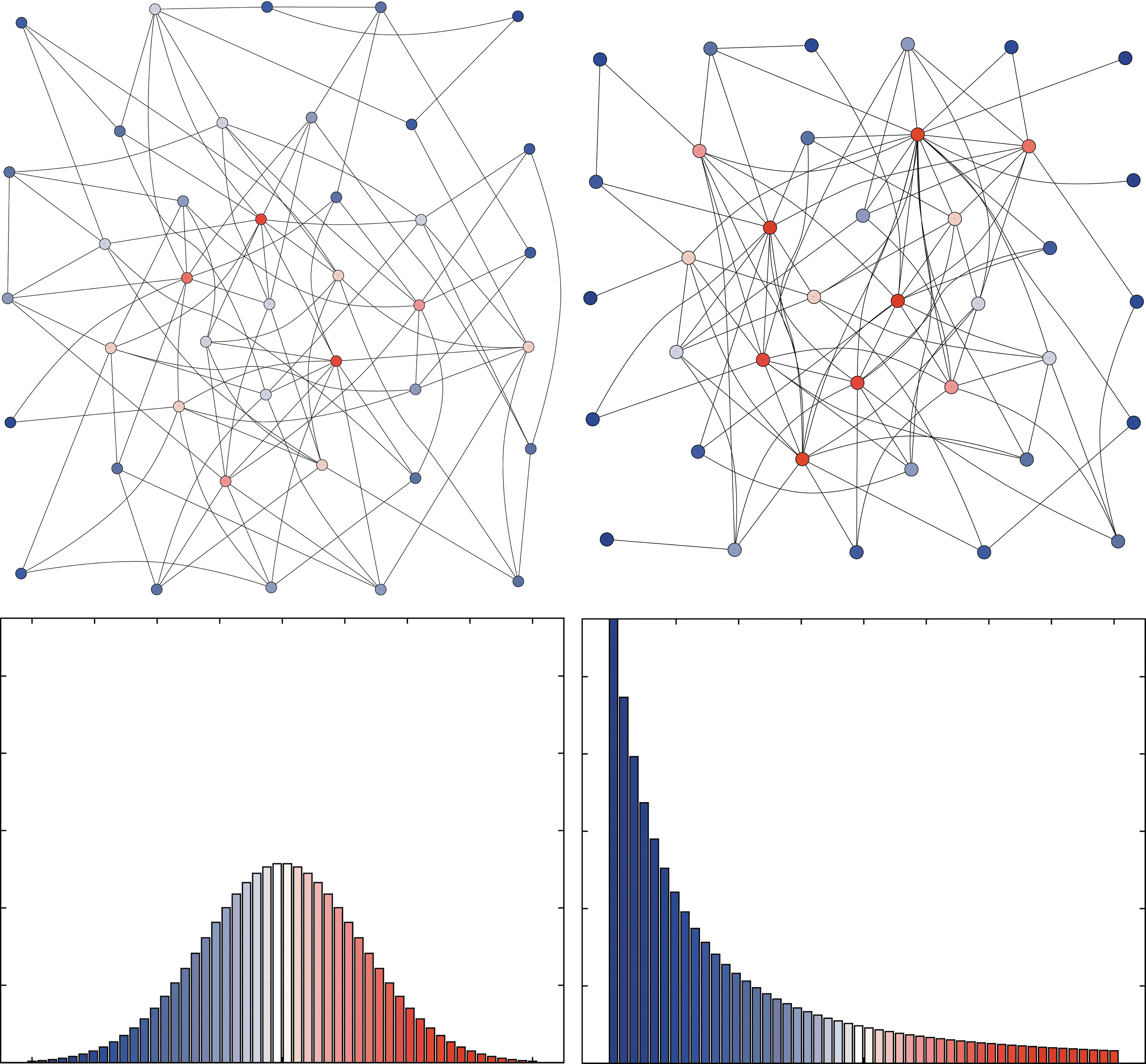
A random network (left) and a scale-free network (right). Node degree is color coded such that red corresponds to high degrees, and blue to low degrees. Note that the scale-free network has a few distinct hubs, whereas the random network has a more even distribution of degrees. The corresponding degree distributions are shown below.
Network algorithms
In the following, we review several graph-based algorithms. We begin with a class of algorithms for large graphs with hundreds or even thousands of nodes. These algorithms perform an analysis of the connectivity matrix and differ in the way in which this is done. Later, we move to algorithms that are designed for smaller graphs with few nodes.
Node selection
Graph-based algorithms require specification of network nodes. In the context of fMRI-based analysis, this usually amounts to some form of presegmentation or parcellation of the imaging data so that each parcel or ROI represents a node. Several authors have proposed and investigated various strategies, and they all agree that this remains a challenging problem (e.g., Smith et al., 2011; Zalesky et al., 2010). No universally accepted parcellation method exists so far, making this point one of the main issues of graph-based analysis techniques.
Zalesky and colleagues (2010) provide a quantitative evaluation of several methods for ROI identification. They found that the overall small-world or scale-free topology remained intact regardless of the spatial scale at which ROIs were defined. However, the quantitative markers of small-worldness changed considerably depending on the spatial scale.
Perhaps, the most frequently used approach is the automated anatomical labeling (AAL), which provides an atlas-based predefined parcellation into 90 anatomical regions (Tzourio-Mazoyer et al., 2002). While this method is easy to use and therefore quite popular, its suitability is often quite problematic. Its main drawback is that the parcellation may be too crude and may fail to adequately represent individual neuroanatomy.
The number of regions of interest may also play a significant role and was recently discussed by Craddock and colleagues (2012). They reported a tradeoff between interpretability and accuracy with regard to the number of ROIs. Fewer than 200 ROIs seemed to make identification of the reported regions easier, while 600 or 1000 ROIs were more accurate in representing functional connectivity patterns. They propose a data-driven parcellation method based on spectral clustering.
Mumford and colleagues (2010) present an interesting algorithm for node selection called “weighted voxel coactivation network analysis”. The main idea is to assign two voxels to the same ROI if their fMRI time series are highly correlated and the voxels they are correlated with are also highly correlated among themselves. This roughly corresponds to the local clustering coefficient explained above.
Centrality mapping
In the following, we will review techniques for assessing hubness or centrality of network nodes. The degree of a node is the sum of its connections or in binary graphs its number. Nodes with high degrees can be assumed to have important roles within their network. Many studies have investigated changes in the node degree in response to changes in the brain state or as a consequence of pathologies (Buckner et al., 2009; Tomasi and Volkow, 2011).
For lack of space, we will not discuss other graph-based measures, and refer the reader to other reviews (e.g., Bullmore and Sporns, 2009) and a test–retest evaluation (Braun et al., 2012). For a comprehensive assessment of a range of centrality measures, see for instance, Zuo and colleagues (2012).
Note that preprocessing strategies may heavily influence results obtained by any of these methods, see also the section Preprocessing strategies. A commonly used procedure in this context is to first parcellate the data space according to some regime as described in the section Node selection. In principle, any of the measures of association described in the section “Measures of association” can be used to define links in the network. However, the most commonly used measure is the pairwise linear correlation between time courses averaged within each parcel. Correlation values are often thresholded so that the connection strength is ignored (Zuo et al., 2012).
Eigenvector centrality mapping
An alternative to degree centrality is eigenvector centrality. It was originally introduced in the field of social network research by Bonacich (1972). A later variant of eigenvector centrality plays a major role in Google's PageRank algorithm [Langville and Meyer (2006)]. Much like node centrality, it favors nodes that have high correlations with many other nodes (see Fig. 4). However, in contrast to node centrality, it specifically favors nodes that are connected to nodes that are themselves central within the network. It is this feature that mimics the preferential treatment effect typical in scale-free networks. As discussed earlier, this effect is caused by positive feedback mechanisms that are essential ingredients of complex systems.
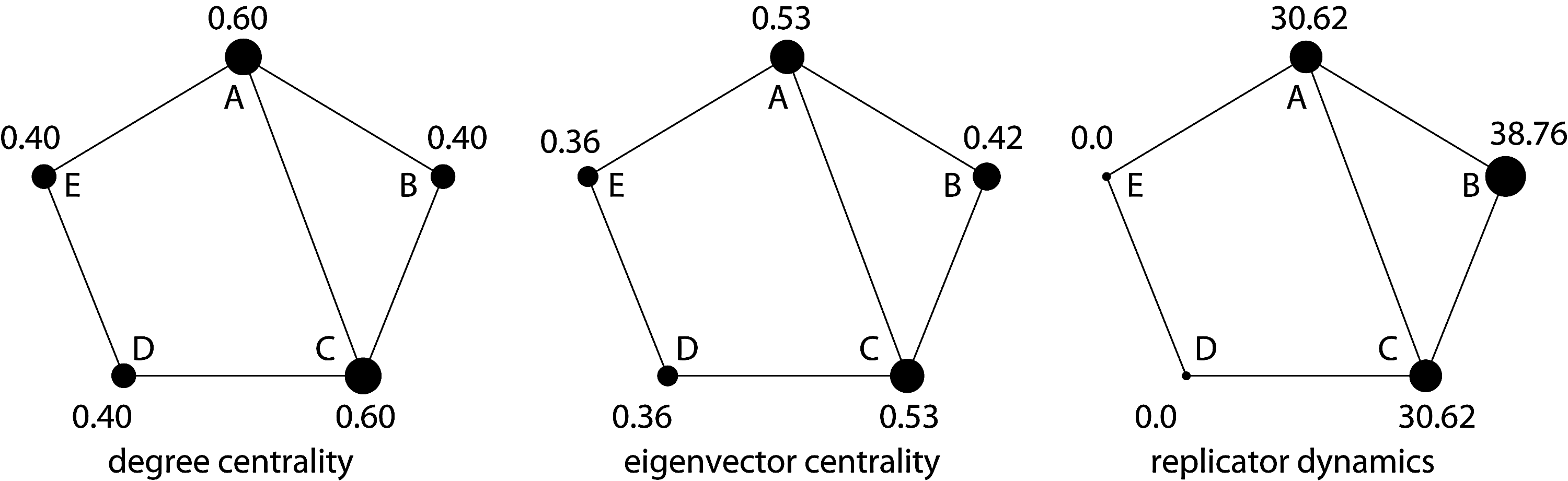
Illustration of centrality measures and replicator dynamics. Nodes A and C are most central in both degree and eigenvector centrality (EC). In degree centrality, nodes B, D, E, are all equal because they all have the same number of connections. However, in eigenvector centrality, B is stronger than D, E because B has connections to two strong nodes, whereas D, E, have only connections to one strong and one weak node. Replicator dynamics identifies the clique structure A, B, C after 100 iterations and sets the other two nodes to zero.
Eigenvector centrality mapping (ECM) was proposed for fMRI data analysis in (Lohmann et al., 2010), and later applied in several other fMRI studies. In its original formulation, the ECM is applied at the voxel level so that each node in the network corresponds to one voxel, and no prior parcellation is required. The mathematical background is as follows. Let A denote an n×n similarity matrix with non-negative values only. The eigenvector centrality xi
of node i is defined as the i-th entry in the eigenvector belonging to the normalized largest eigenvalue of A. Let λ be the largest eigenvalue and x the corresponding eigenvector, then
with proportionality factor μ=1/λ so that xi is proportional to the sum of similarity scores of all nodes connected to it. Thus, nodes that are well connected to other well-connected nodes are favored.
Eigenvector centrality is related to PCA in that both methods are based on eigenvector decompositions of similarity matrices. However, the difference is that the first principal component is really a projection of the data along the direction of the first eigenvector, not the eigenvector itself (see description of PCA in the section “Principal component analysis”). Furthermore, PCA differs from ECM in that it is based on linear correlations as a similarity metric. However, linear correlations may be negative so that the first principal component is not uniquely defined because of possible multiplicities of eigenvalues. Other metrics such as spectral coherence, for example, are not customary with PCA.
Many algorithms for computing eigenvectors of symmetric matrices are known. In the present context, it suffices to find the eigenvector belonging to the largest eigenvalue. For this special case, the power iteration method (Golub and van Loan, 1996, 405ff) is one of the most efficient.
Replicator dynamics
Let us now discuss another approach for analyzing the network structure. Here, we want to identify networks of brain activity such that all members that belong to the same network interact with each other. In such a network, every element is close to every other element. Such networks can be detected using a concept well known in theoretical biology called “replicator dynamics” (RD). RD describes the growth of populations consisting of several species that interact with each other [Hofbauer and Sigmund (1988) and Schuster and Sigmund (1983)]. It is described by the following equation known as the replicator equation:
where xi
, i=1,…n are membership values for each of the n elements, and the n×n matrix A is a similarity matrix whose elements must be non-negative, and k denotes the iteration step. Initially, at the first iteration k=0, all elements i=1,…n have the same weight
RD was first applied to fMRI data in Lohmann and Bohn (2002), and later, also in Müller and colleagues (2007) and Neumann and colleagues (2005, 2006). Recently, an extension to group level analysis was proposed by Ng and colleagues (2012). RD shares some similarities with ECM. Both RD and ECM highlight networks in which interaction among highly weighted elements is favored, and RD was shown to yield scale-free networks (Santos et al., 2006).
See Figure 4 for an illustration of centrality measures and RD.
Dynamic causal modeling
Dynamic causal modeling (DCM) (Friston, 2011; Friston et al., 2003) is a technique designed to investigate the influence between brain areas using time series data measured by fMRI or EEG/MEG. DCM is a model-based method in which a set of user-specified directed graphs represent possible arrangements of functional connections between predefined brain areas. Based on a model fit and parsimony, the best model is chosen and taken to be the winner. DCM is typically applied to small networks consisting of a handful of nodes.
At the heart of DCM is the following system of differential equations, which expresses temporal dynamics of functional connections represented by their corresponding matrices:
with matrix A representing intrinsic connectivity among n brain regions, matrices Bj , j=1,…m representing connectivity modulated by m experimental manipulations, and matrix C representing influences of inputs on the neural activity. The brain regions whose connections we want to investigate are usually represented by peak activations obtained by a standard GLM-based analysis. The transformation from neuronal states to the observed hemodynamic response is modeled via the Balloon-Windkessel model (Buxton et al., 1998). A dynamic causal model is generative in that it generates synthetic time courses, which are subsequently matched against the measured data. Several extensions of this method have been proposed (Li et al., 2011; Penny et al., 2010; Stephan et al., 2008). For a review, see Friston (2011).
The validity of DCM was recently debated in a series of articles (Breakspear, in press; Friston et al., in press; Lohmann et al., 2012; Lohmann et al., in press). The main points of critique were related to combinatorial explosion, the validity of the model selection procedure, and problems with respect to model validation.
The reasons underlying the problems of DCM may be seen in view of our introductory remarks about complex systems. Complex systems are characterized by a large number of constituents, and complexity arises out of the multitude of nonlinear interactions among those many agents. Small systems with few constituents cannot be complex, even though they may be highly complicated (Baranger, 2012; Rickles et al., 2007). As was recently shown, even very simple paradigms may activate large portions of the brain (Gonzalez-Castillo et al., 2012), so that insufficient model size of DCMs may in fact be one of the key issues to be investigated in this context.
In this context, it is important to note the difference between generative and discriminative models. Generative models such as DCMs should provide a full probabilistic description of all variables in the model, whereas discriminative models only need to provide a model for some target variables conditional on the observed variables (Ng and Jordan, 2001). In other words, generative models are much more ambitious, and we would expect a generative model of a brain function to reproduce at least some of its most salient features reflecting complexity such as large-scale spatial patterns of activation. We cannot expect a model with a handful of nodes to yield a realistic picture of cognitive and, hence, complex functions.
Bayesian networks
Bayesian networks have been proposed as a tool to estimate interdependencies between brain regions from fMRI time series or coactivation patterns. This idea rests upon the concept of conditional probabilities. Consider, for example, the activation of two functional brain regions A and B. If activation of region B depends on the activation of region A, then the conditional probability of activation of B given A will be greater than the conditional probability of activation of A given B: P (B|A)>P (A|B). Conditional probabilities can thus be utilized to estimate a pairwise directionality between brain regions (Patel et al., 2006).
Bayesian networks extend this notion, representing a set of random variables and their full probabilistic dependence structure. More formally, a Bayesian network is a directed acyclic graph G that comprises • a set of nodes or vertices V in a one-to-one correspondence with a set of random variables • a set of directed links or edges connecting these nodes.
Each variable Xi
is assigned a conditional probability distribution P (xi|
The structure of a Bayesian network and hence, the interdependencies between brain regions can be learned from observational data, in our context from the covariance matrix of fMRI time series. For a discussion and comparison of the various network learning techniques see, for example, Chickering and colleagues (1995), Pearl (2000), Spirtes and colleagues (2000), and Steyvers and colleagues (2003). One caveat of structure learning is that some of the links typically remain undirected due to the statistical equivalence of several networks underlying the observed data (Pearl, 2009). Despite this limitation, Smith and colleagues (2011) demonstrated in an extensive simulation assessing the suitability of different network modeling approaches for the detection of network connections and their directionality that Bayesian network techniques scored among the highest when applied to good quality fMRI data.
This technique is typically applied to small networks with few numbers of nodes. However, since it is not a generative modeling approach, lack of complexity is not an issue, so that here we do not have the problem inherent in DCM.
Importantly, the use of Bayesian networks for inferring directed functional brain networks can be extended to data obtained from several independently performed fMRI experiments (Laird et al., 2005; Neumann et al., 2010, 2011). On this so-called meta-analysis level, coactivation patterns for several brain regions rather than the covariance structure of individual fMRI time series serve as observational data. This way, inference on possible brain network structures can be grounded on data collected across multiple sources.
Such meta-analytic techniques are among the big data research directions that we mentioned in the introduction. “More is different” is particularly true for the technique described in (Neumann et al., 2010) because Bayesian network estimation requires very large amounts of data. It becomes unreliable otherwise.
Conclusion
We have reviewed a broad collection of recent approaches for fMRI data analysis. These approaches are either directly or indirectly inspired by three major developments that have begun to dominate the field, namely, complex systems theory, data-intensive research, and ultra-high field MRI. In one way or other, they all fall under the heading “more is different.” However, we should note that sometimes, “more may be less” because more data does not necessarily imply more knowledge.
Open issues
A number of issues are still open for debate. In particular, we need to be aware of the fact that preprocessing strategies have a major impact on our results, and it is presently not clear which strategies are best or even legitimate. In general, one should always try to preserve as much as possible of the original data, and refrain from a rigorous alteration of the data. In this case, less may often be better. Another open point is the choice of free parameters. Some techniques, for instance, require some form of thresholding, and it is often unclear how this should be done.
The most pressing concern may perhaps be the difficulty in validation and interpretation of results. Since we do not have access to any form of ground truth, it is often next to impossible to validate or even to interpret the results that come out of our new algorithms. How do we know that a new algorithm is correct and suitable? Currently, the standard procedure is to apply it to our data and hope to find something familiar. Of course, this is not a very satisfactory way of dealing with this problem. There is clearly a need to specify more principled criteria by which to judge the suitability of an algorithm. One possibility may be to check for reproducibility of results (Lange et al., 1999; Zuo et al., 2012) or to provide some form of test bed against which algorithms should be checked. In any case, it is essential to be aware not only of the possibilities, but also of the limitations of fMRI to avoid an overinterpretation of results (Logothetis, 2008).
A similar problem relates to the estimation of statistical significance. The novel techniques reported in this article often require new forms of statistical inference. The inference methods that are presently available were originally designed for univariate GLM-based studies. Simply transferring these methods to the multivariate domain is often not legitimate. New inference methods are clearly needed (see for instance, Stelzer et al., 2012).
Future trends
The complex system inside our brain changes over time. Understanding the dynamics of the intricate patterns that are formed by this complex system will be one of the most challenging tasks in the future. Increasing the sensitivity to these spatiotemporal patterns should be a key element of the future algorithm design (Bressler and Menon, 2010; Hasson and Honey, 2012).
We predict that future brain analysis methods will highlight the view of the brain as a complex system, and therefore move away from limitations posed by univariate, or small-scale multivariate algorithms. This entails that in the future, the focus will shift toward identification and analysis of emergent large-scale spatiotemporal patterns that provide a more realistic picture of brain function. After all, the hallmark of cognitive processes is the formation of transient coalitions of brain areas that collaborate to perform a task. In conclusion, in the future, we will need massively multivariate algorithms because “more is different.”
Footnotes
Acknowledgments
J.N.'s work is supported by the Federal Ministry of Education and Research (BMBF), Germany, FKZ: 01EO1001.
Author Disclosure Statement
No competing financial interest exists.