
Abstract
Inferences of strong modular and hierarchical structure from some cortical network studies conflict with the broadly isotropic homogeneous connectivity that has been found to a first approximation in classical anatomical studies. This conflict is resolved via consideration of the geometry of the cortex. A new geometrically based connection matrix (CM) visualization method is used to better compare experimental CMs with model CMs and thereby minimize appearance of artifacts. Model networks based on spherical geometry containing similar isotropic, homogeneous connection distributions to the experiment are shown to reproduce, interrelate, and explain key properties of experimentally derived networks, such as clustering coefficient (CC), path length, mean degree, and modularity score, using only two parameters that are fitted to an experimental spatial connectivity distribution. A greater CC in the experiment than the model indicates that, while isotropy and homogeneity of connections is a good first approximation, connections at shorter range may exhibit additional perturbations that increase clustering. These geometrically based models provide a comparative framework to assist in the next stage of revealing and analyzing anisotropic and/or inhomogeneous connections in data and their effects on network properties and visualization.
Introduction
The cortex is extremely complex anatomically and performs many highly specialized functions. It is considered that to implement such a diverse set of capabilities, there should exist highly specialized connections within the white matter of the cortex; however, the amount of specialization and the connective architecture in general is not well understood. Concepts such as modularity and hierarchy currently guide much research in the area of cortical networks, but the modularity and hierarchy of cortical connectivity cannot yet be described conclusively (Meunier et al., 2009, 2010; Zhou et al., 2006). Here, hierarchy refers to cases in which a collection of modules are successively grouped together to form larger modules with decreasing connection strength between them. Moreover, some types of anatomical studies have observed that connectivity is isotropic (rotationally invariant) and homogeneous (translationally invariant) across the cortex to a first approximation (Braitenberg and Schüz, 1998; Kaiser et al., 2009; Schüz and Braitenberg, 2002; Schüz et al., 2006), and such observations have been successfully applied to work in areas such as mean-field modeling of brain activity (Deco et al., 2008). Conversely, other types of connectivity have also been observed, particularly in fine-scale horizontal connectivity such as patchy connectivity in the visual cortex (Rockland and Lund, 1983).
The observations of broad isotropy and homogeneity cited earlier appear to conflict with inferences of extensive modularity and hierarchy. Are both sets of observations related and can, therefore, be reconciled? Can the broad isotropy and homogeneity be disentangled from other anisotropic and/or inhomogeneous connectivity; modular, hierarchical, or otherwise?
In addition to modular and hierarchical structure, network analysis has identified a variety of general principles that apply to cortical networks, with two key features being the small-world properties of simultaneous high clustering and low path length (Bullmore and Bassett, 2011; Bullmore and Sporns, 2009; Meunier et al., 2010; Sporns, 2010; Zalesky et al., 2010). However, a list of individual features does not provide an integrated understanding of connectivity; the relations between such properties need to be developed through modeling and reconciled with other known properties of the brain, especially its functions and basic physical properties such as its geometry. One approach to synthesizing this knowledge and answering such questions is to investigate strong links between underlying physical features of the cortex and these observed network properties (da F Costa et al., 2007; Robinson et al., 2009). Models based on consideration of simple physical quantities with a few starting assumptions should be able to provide insights by connecting physical quantities with observed properties of cortical networks.
The connections of the cortex and the cortical regions they link are, of course, embedded in three-dimensional (3D) space. The geometrical arrangement of regions and connections that evolution has produced is likely to have a strong impact on the network architecture of the cortex. Surprisingly, although the spatial arrangement of cortical connections has been widely studied (da F Costa et al., 2007; Robinson et al., 2009; Voges et al., 2007), incorporation into cortical network modeling is only now beginning in earnest. In particular, there has been significant focus on the idea of wiring length minimization in the brain. This has been studied in Caenorhabditis elegans (Varshney et al., 2011) as well as in the macaque (Kaiser and Hilgetag, 2006). These studies have shown that wiring lengths tends to be small, but could be reduced further. In Bullmore and Sporns (2012), it has been suggested that the brain economy makes trade-offs between costs, such as those associated with wiring length and topological network benefits. Investigations into functional brain networks have shown that distance-based connectivity partly accounts for observed functional connectivity, but additional mechanisms such as preferential attachment produce a better match to data (V'ertes et al., 2012). However, such models are abstracted and well removed from underlying mechanisms and, hence, difficult to interpret in terms of dynamics operating on an underlying structural network, as well as measurement procedures such as global signal regression that heavily influence correlation and, hence, functional connectivity results (Robinson, 2012). Instead, developing models of structural connectivity based on anatomy and physiology, and applying a consistent theory of cortical dynamics would produce much greater insights into the properties of functional networks and their relation to the underlying structural networks (Knock et al., 2009). Good models of structural connectivity highlighting the dominant influences on structural connectivity are critical to such studies.
Recently, Henderson and Robinson (2011) compared the properties of a simple network model consisting of a planar two-dimensional (2D) sheet of nodes connected to nearest neighbors to a low-resolution experimental cat cortical network. This idealized model was the simplest model to enable qualitative understanding of how the broad features of two dimensionality and local connectivity combine to produce network properties that are similar to those found in experimental cortical networks. While this model qualitatively supports a strong influence of geometry on cortical networks, a greater degree of cortical specificity, for example, curvature and closed topology, is required for detailed and quantitative analysis and comparison to higher-resolution experimental data.
In this article, we explore a geometric model that includes realistic isotropic and homogeneous features, extending beyond the work of Henderson and Robinson (2011). Specifically, we aim at investigating geometric isotropic homogeneity in cortical connectivity as a step toward uncovering how such underlying principles can give rise to observed cortical network properties and then inferring which properties require other anisotropic, inhomogeneous connectivity. To do this, we introduce a more brain-like model geometry than previously used by constructing a spherical spatial distribution of nodes that can be more directly compared with experimental data than the planar model in Henderson and Robinson (2011), and an exponentially decaying probability of connection kernel, modeled on experimental data. Once results for these models have been established, new models may be investigated to understand the impact of cortical convolutions.
The resulting networks are found to reproduce many features of experimental connection data despite using no free parameters. Two geometrically based indexing methods are presented that allow a more direct and informative visual comparison as well as potential for simpler mathematical manipulation and interpretation. Quantitatively, both model and experimental networks have very similar clustering coefficient (CC), though the model CC is slightly lower than observed in experimental data. The similarity in mean degree, path length, and modularity is a significant improvement compared with planar and hierarchical models (Henderson and Robinson, 2011; Robinson et al., 2009), despite the model lacking any modularity. These results indicate that a base homogeneous, local connectivity is sufficient to produce observed mean degree, path length, and modularity properties, but we find that additional modification and specialized short-range structures are required to increase the CC. Thus, this model connects geometric and network properties of the cortex, showing that issues of isotropy, homogeneity, and modularity are closely related in realistic cortical geometry. This provides a framework to enable future work to assess the effect on network properties arising from other anisotropic and/or inhomogeneous structures. These results are also likely to be applicable to a wide range of other noncortical networks embedded in 2D surfaces, including networks of transport, ecological, economic, and other interactions (Barthelemy, 2011; Bullock and Geard, 2010; Henderson and Robinson, 2011).
Methods
Here, we present the methods of construction and visualization of the network models used in the later analysis, as well as a description of the network measures applied to them.
Construction of 2D spherical cortical network model
The cortex has two simple features that we use as the basis for our network model. First, the overall geometric structure of the cortex is that it comprises a thin 2D folded sheet of neuronal cell bodies (gray matter) overlaid on bundles of connections (white matter). Second, the white matter is predominantly arranged to link spatially close regions of gray matter (Braitenberg and Schüz, 1998; Kaiser et al., 2009). As is typical in network modeling of the cortex, the gray matter forms the nodes of the cortical network and white matter forms the edges. There are many short-range connections within the gray matter itself, typically much smaller than individual nodes considered in current experiments; so, we do not specifically model these here (Braitenberg and Schüz, 1998).
In order to probe connection properties due to isotropic, homogeneous connections in the cortex, we use an isotropic, homogeneous model in which each node is identical and there are no special nodes. Henderson and Robinson (2011) used a 2D plane geometry as the basis for such a cortical network model. This is suitable as a first approximation or as a model of a patch of cortex, but curvature and more realistic boundary conditions need to be considered, especially for low-resolution whole-cortex networks in which boundary effects are significant. Spherical topologies are often used to represent the cortex (Yotter et al., 2011). Here, a spherical topology is used as a closer approximation to a whole cortex or hemisphere when comparing with experimental cortical networks. In future, models with more complex geometry will be used to understand the impact of detailed cortical convolutions.
Generation of spherical node distribution
The following procedure is used to produce a set of isotropic, homogeneous node locations that are distributed evenly over the surface of a sphere of unit radius, as illustrated in Figure 1. A spherical surface is initially approximated using the vertexes of a regular icosahedron (12 vertexes, 20 equilateral triangular faces). Each face is repeatedly replaced by four smaller equilateral triangles with their vertexes on the spherical surface (i.e., displaced outward from the plane of the original triangle), until the desired number of vertexes is realized, thus yielding a mesh of equilateral triangles that approximates a spherical surface. At successive iterations, i=1, 2, 3…the method produces 12, 42, 162, 642, 2562,…,10×4 i−1+2,…vertexes, with vertex positions used as node positions in the inflated-sphere representation of the cortex. When a required network size differs from these values, a subset of these nodes is randomly chosen.
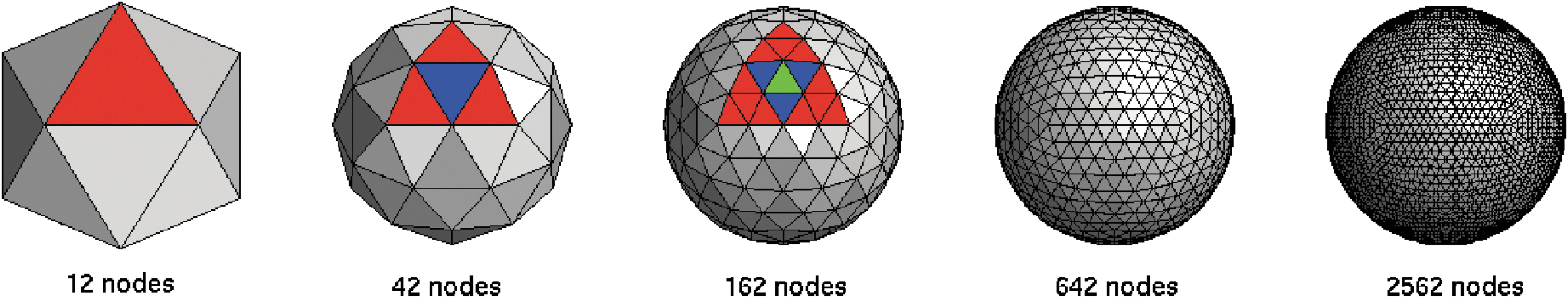
Construction of spherical distribution of nodes. Left: Beginning with a regular icosahedron (12 vertexes, 20 equilateral triangular faces), faces are repeatedly replaced by 4 smaller equilateral triangles with their vertexes on the spherical surface. Two iterations are highlighted for one starting triangle with the colors indicating each iteration. The red triangle on the left is divided into 4 smaller triangles (3 red, 1 blue) on the first iteration, the 4 triangles are then divided into 16 smaller triangles (12 red, 3 blue, 1 green) on the second iteration, and so on.
Connection kernels
Here, we describe how the connection kernel is used to form a network from the spherical distribution of nodes. We aim at generating and analyzing the properties of a network containing brain-like local isotropic, homogeneous connectivity. Then, further, we aim at identifying differences from experimental data to highlight the importance of other anisotropic and/or inhomogeneous connectivity. To do so, we introduce four specific models of connectivity, as discussed next. We mainly focus analysis on the third model, and use the others for comparison, as network properties are more easily interpreted via comparison to other networks with known characteristics. The four models are as follows:
Model 1, Random Network: Each pair of nodes is connected randomly with connection probability p. This distribution is unrealistic as a model of an actual cortex, but is a well understood, standard network (Sporns, 2010) and is, thus, used here for comparison with other more realistic distributions. Geometry does not influence the architecture of a network with random connectivity, because the spatial distribution of nodes does not affect the probability of connection.
Model 2, Nearest Neighbor: A nearest neighbor connection kernel is applied at each node that connects it exclusively to all nodes within Euclidean distance r. This was used by Henderson and Robinson (2011) and provides a simple, easily interpreted model that captures fundamental local isotropic, homogeneous connectivity properties of data networks.
Model 3, Single Exponential: A connection kernel is modeled on data to approximate brain-like local isotropic, homogeneous connectivity that decays with distance. Connection data exist for cat and macaque cortexes (Felleman and Van Essen, 1991; Scannell et al., 1995); however, the parcellations used contain relatively few areas and they have a high degree of nonuniformity in node geometry. This makes them difficult to compare directly with this model (Butts, 2009; Wang et al., 2009). In contrast, the diffusion spectrum MRI (DSI) connectivity data for the human cortex published by Hagmann et al. (2008) have significantly higher resolution and greater uniformity in parcellation, so we use them here. The unweighted connection matrix (CM) is shown in Figure 2a, indexed as in Hagmann et al. (2008). The distributions of connections with Euclidean spatial separation r of nodes and fiber lengths are shown in Figure 3. Note that the spatial separations are straight line distances and do not account for curvature of the cortical surface or other effects. Both the Euclidean distance and fiber length distributions in Figure 3 have a similar functional form. This justifies the use of Euclidean distance as the governing parameter for connectivity in the models (We have also tested similar models which use distances on the spherical surface and have found that these produce similar results, see Supplementary Fig. S1; Supplementary Data are available online at
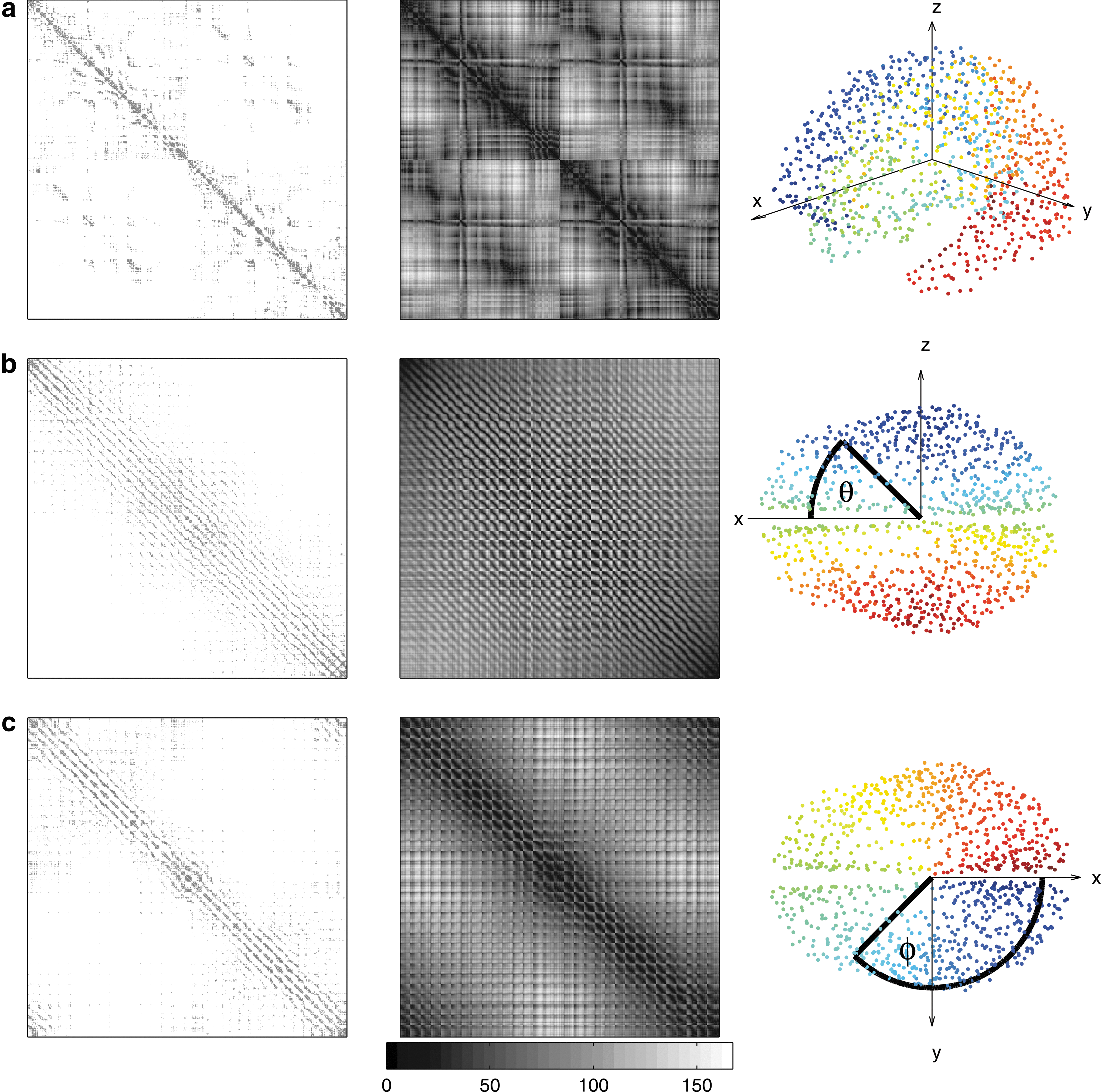
Comparison of human DSI experimental unweighted connectivity data (Hagmann et al., 2008) with each row having a different indexing method. First column: Human DSI experimental unweighted CM with
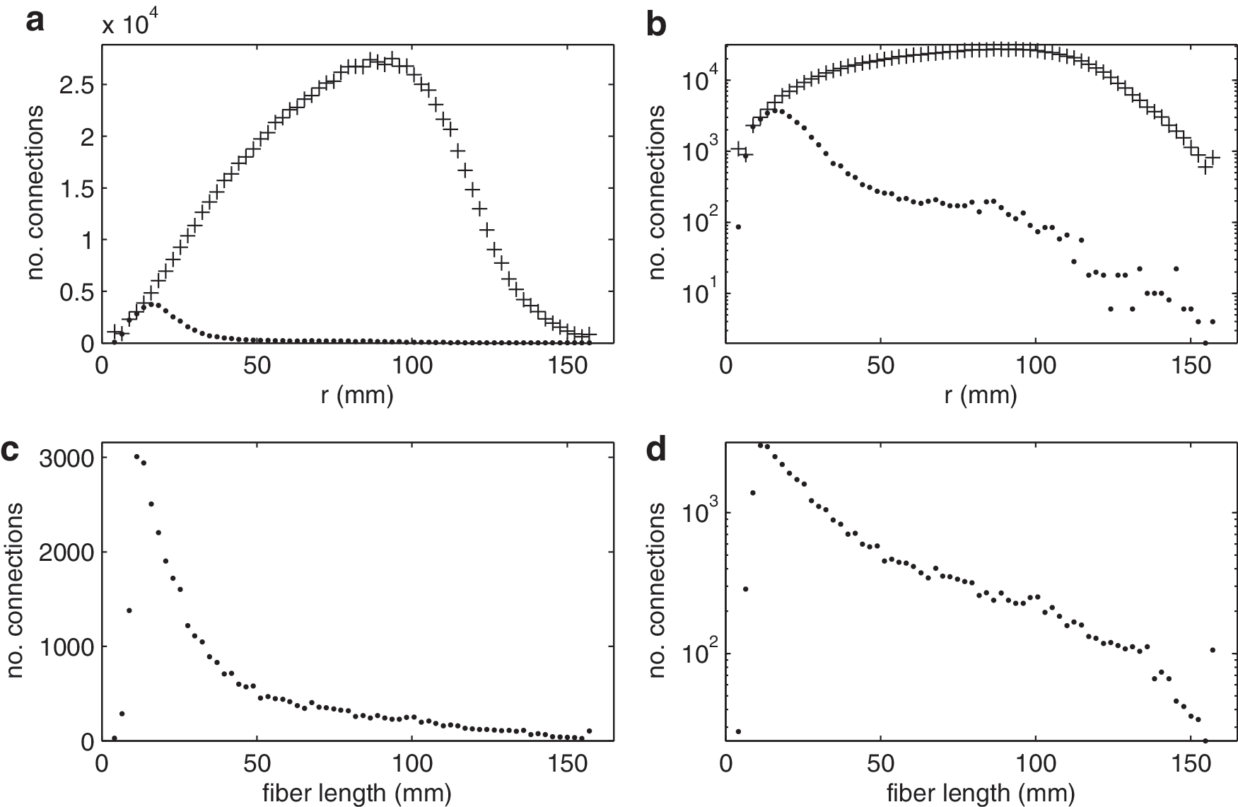
Human DSI connection data spatial distributions. Frames
Human DSI connection data spatial distributions. Frames
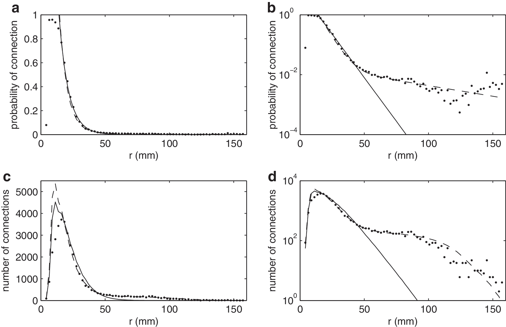
We approximate the connectivity distribution in Figure 4a and b with a simple exponentially decaying probability of connection. A network with an exponential probability of connection was previously studied in the context of growing cortical networks (Kaiser and Hilgetag, 2004; Newman and Girvan, 2004); however, this model was somewhat unrealistic in its highly inhomogeneous spatial positioning of nodes, and involved two free parameters, whereas the present models have no free parameters. Mathematically, each pair of nodes in the model has probability of connection
where C and r 0 are constants fitted to DSI data (Fig. 4), and r is the Euclidean separation of nodes.
In the case of a continuous distribution of nodes on the sphere, integrating around a polar angle on the spherical surface gives the connection density
where R is the radius of the sphere. This displays similar features to those observed in Figures 3 and 4; a rapidly increasing number of connections at small node separation, which decays at large r, thus capturing the vast majority of connections. At ranges r>50 mm, the curve corresponding to Equation (2) decreases faster than the experimental one. The absence of these longer-range connections in this model serves to highlight their importance in determining network properties on a comparison of the model to experimental data and/or Model 4 given next.
Model 4, Double Exponential: The longer-range connections present in data can be modeled by adding a second exponential to the probability of connection used in Model 3. Mathematically, each pair of nodes in the model then has probability of connection
where Cs
and rs
are constants fitted to DSI data for a short-range exponential distribution, Cl
and rl
are fitted constants for a long-range exponential distribution (Fig. 4), and r is the Euclidean separation of nodes. Analogously to Equation (2), the r-dependent connection density is
The longer-range connections in DSI data are rare and, hence, appear anisotropically and inhomogeneously distributed; however, it is not currently known how much anisotropy and/or inhomogeneity can be attributed to artifacts from measurement where detection of certain types of connections is biased (Bihan et al., 2006) or factors are involved in actual connectivity. Some potential sources of anisotropy and inhomogeneity in actual connectivity are (i) shot noise in which a homogeneous isotropic connectivity distribution contains a region of low probability, resulting in only a few scattered connections forming (ii) more detailed anisotropic and/or inhomogeneous geometry (such as lobe structure or cortical folding), resulting in anisotropic and/or inhomogeneous connectivity, or (iii) highly specialized connections which are separate from cortex-wide connectivity distributions; for example, one that might form a network backbone architecture (Hagmann et al., 2008).
CM indexing
CMs are widely used to visualize connectivity data. In a CM, the indexes of the matrix represent each individual node in the network. Nonzero entries within the matrix indicate the presence of a connection between the two nodes which index that location.
To visualize connectivity data from experiments or the models described eartlier in the form of a CM, the two dimensions of the gray matter sheet need to be placed in a one-dimensional (1D) index sequence. By considering the geometry of the cortex, experimental CMs can be usefully reindexed in a manner that reveals important structure and can be replicated in the model for comparison. We present a simple procedure for indexing that involves consideration of the geometrical location of nodes. Nodes are divided into angular bands based on spherical coordinates and indexed in order of θ (azimuth angle) or φ (polar angle). The spherical coordinates of each node are calculated using the mean position of all nodes as the origin. The choice of x, y, and z axes is arbitrary; different choices produce CMs with the same broad structure, but with different fine-scale features. Different axes may be used to highlight different features such as front–back or left–right connectivity within the CM. Once a coordinate system is chosen, nodes are sorted into bands of θ (azimuth angle) or φ (polar angle) with equal numbers of nodes in each band, as shown in Figure 2.
The choice of node index order in a CM does not alter the connectivity information contained in the matrix; however, it affects the CM structure and impacts visualization and some types of mathematical manipulation of network connectivity data, as detailed next.
The nodes in the previously published form of the DSI CM were indexed in each hemisphere, beginning at the frontal lobe, then moving successively through the parietal, occipital, and temporal lobes, as shown in Figure 2a (Hagmann et al., 2008). While the CM in this format clearly has structure and is not random, it is not immediately obvious what that structure is and, importantly, it is not clear how this translates back to the structure of the cortex. In addition, the ordering of CM indexes is based on inhomogeneous geometrical features that are found in real cortexes, but which do not typically exist in models; this complicates finding equivalent indexing in models and a direct visual comparison between model and data.
Indexing has a vital role in visualizing the network, and its effect in shaping apparent CM structure can be as strong as the connection data itself. For example, the CMs shown in Figure 2a and b have a very different structure, despite identical underlying networks. A standard indexing technique does not exist for cortical networks, so published experimental CMs are difficult to compare visually despite qualitative conclusions sometimes being drawn from such comparisons, for example, (Johansen-Berg et al., 2004). However, most published CMs appear to be pregrouped anatomically through grouping of associated functional processing areas; for example, visual/auditory, producing a roughly block diagonal form (Felleman and Van Essen, 1991; Scannell et al., 1995). These experimental CMs can at first appear to contain structures such as modules and hubs; however, these observed structures are subject to artefacts introduced via choice of index ordering and may be artificial, or enhanced or reduced from those that actually exist in the cortex (Henderson and Robinson, 2011). It is, thus, necessary to be careful when selecting a method of ordering indexes so as to be able to visually compare different CMs, reveal certain desired structures, and recognize any misleading artefacts that result from indexing or otherwise. This highlights the possibility of arriving at flawed interpretations of network structure from an observation of CMs alone and raises the question of which method of index ordering should be used as well as the need for labeling independent measures.
Apart from visual interpretation, for the purposes of calculations, the choice of ordering nodes can produce CMs with certain forms that simplify, improve, or speed up calculations and enable use of mathematical theorems. For example, as shown in the next section, in the case of predominantly locally connected or modular networks, the nodes can be ordered in such a way so as to produce Toeplitz-like matrices (a matrix in which the descending diagonals from left to right all contain the same entries), and circulant-like matrices (special types of Toeplitz matrices in which each row/column is a cyclic permutation of the previous row/column) (Gray, 2005) whose eigenvalues can be easily computed and other useful results apply (Gray, 2005; Sarkar et al., 2013). In addition, many existing algorithms, such as those for detecting modules, have differing outputs that depend on the initial CM format; so, CM node ordering can be important (Blondel et al., 2008). Using multiple runs with different, random indexing is often used to find an ensemble mean algorithm output. However, a decision to use a set of random indexes could also bias results. For example, the mean output of an ensemble of randomly indexed CM inputs neither necessarily produces the most suitable modular division of a network, nor removes the fact that there is variation, and, hence, uncertainty in the interpretation of the output of a given algorithm for a given network. Carefully indexed CM inputs may, thus, produce superior results.
Network measures
Network structure is difficult to assess visually; so, quantitative visualization-independent measures applied to both the network in question and a range of comparison networks are required. In this article, only undirected networks are considered. We compare models and experimental data with the following commonly used network measures that highlight key properties of networks (Bullmore and Sporns, 2009; Zalesky et al., 2010).
(i) Mean degree
(ii) Path length L: the fewest connections linking a pair of nodes in the network, averaged over all pairs of nodes in the network. This is not a geometrical length; it relates to numbers of synapses or processing steps between nodes.
(iii) CC: for a single node, the ratio of actual number of connections between its neighboring nodes to the maximum number possible. Again, we consider the average compared with all nodes in the network.
(iv) Modularity Q: one of the key aims of investigation into cortical network architecture is to quantify the possible presence of modules; groups of nodes that connect strongly to each other and less strongly to other groups. The modularity of a network is often quantified by dividing the network into a set of distinct modules, then comparing the number of actual intramodule connections to the number expected if all the connections were redistributed randomly, subject to maintaining the network's degree distribution. Mathematically, this is expressed as
where A is the CM of the network, m is the total number of connections in the network
Results and Discussion
The network models presented in the Methods section are analyzed and discussed next in the context of the following motivating questions: What is the underlying architecture of cortical networks? How can this be accurately and precisely described? What do simple geometrical observations of the cortex imply about its network architecture? To what extent can the observed properties of cortical networks be attributed to isotropic, homogeneous connectivity and to what extent are they due to anisotropic and/or inhomogeneous connectivity?
CM visualization
Visualization of complex connectivity data can be useful in guiding intuition and identifying interesting features in data for further analysis if done carefully. CMs are a common way of visualizing connectivity data; however, as described earlier, the CM should be constructed appropriately to reveal different structures and visualization-independent measures used in conjunction. The indexing methods described here reveal the geometric pattern of short-range connections that dominate the data and models; hence, they are useful in interpreting the data in many cases. However, there is no single indexing method that is universally better than others, as the most suitable method will depend on which aspects of the connectivity the visualization intends to focus on, as different methods focus on different aspects, or on the details of an algorithm to be applied to the CM. In choosing a visualization, it is important to be aware of any artefact structure that is produced in the CM, but is not representative of the structure of the underlying network.
We now describe how a broad geometric connectivity pattern, local connectivity, can be visualized in the DSI CM. Figure 2 shows the DSI CM with its published indexing as well as indexing using the spherical angle technique from the Methods section. The distances between nodes are shown using distance matrices (DMs) containing spatial Cartesian distances between nodes in the second columns of Figure 2. This indexing elucidates at least one structural property of the CMs and DMs: periodic bands of connections along the diagonal. The periodic structure arises from reconfiguring the cortex's two dimensions into a 1D index sequence. Each period corresponds to a band of azimuth or polar angles, depending on indexing, with period equal to the number of nodes allocated to each band. Even though connecting fibers do not take straight line paths between cortical areas, by comparing the bands of connections in the CMs in Figure 2b and c with the bands of short distances between nodes in their corresponding DMs, these bands indicate that local connectivity dominates the structure of the CM, with the same band structure observed in both the DM and the CM.
These DSI CMs in Figure 2b and c are broadly uniform in structure. Note that the matrices do not visually appear to have any obvious modular or hierarchical structure. In comparison, with the published indexing technique, Figure 2a appears to have some block diagonal modular structure. This highlights the potential errors inherent in forming impressions of network structure from a visual observation of CMs alone and the need for careful interpretation of the CM indexing order, as well as the calculation of indexing-independent network metrics, to reveal information about network structure.
In particular, this implies that apparent modular and/or hierarchical structures in CMs can be misleading, and the dominant connectivity may yet be isotropic and homogeneous (Henderson and Robinson, 2011) (this still permits some anisotropy and/or inhomogeneity to be overlaid, which could yield additional modular and/or hierarchical structure).
Indexing by azimuth angle produces a CM that is approximately Toeplitz or block Toeplitz (Gray, 2005) as in Figure 2b with diagonal stripes from top left to bottom right, and in the case of the polar angle indexing as in Figure 2c, approximately circulant or block circulant (Gray, 2005) with descending diagonals as well as a cyclic structure containing diagonals in the top right and bottom left corners of each CM. The Toeplitz/circulant component of the matrices roughly represents an average connection kernel. Homogeneous and inhomogeneous connectivity could potentially be differentiated by extracting the Toeplitz/circulant component of the matrices. This could be achieved through subtraction of an average Toeplitz/circulant component or by removal of connections with distances below a threshold; however, this is beyond the scope of the present article.
Given that we have used geometry to define an indexing technique with a simple geometric interpretation, the experimental CMs are able to be broadly compared visually with model CMs. The DSI data CM in Figure 5a and model CMs in Figure 5b–f have a similar structure, indicating that local connectivity in two dimensions is an important feature of cortical connectivity. A closer examination of Figure 2 reveals some interesting inhomogeneous features in the DSI CMs. Areas of spatial homogeneity in the distribution of nodes and the cortical surface produce corresponding regions of uniform diagonal structure in the DM, because nodes are equally separated in space. Deviation from this uniform structure in the same parts of the CM implies connective anisotropy and/or inhomogeneity in that area. Areas of inhomogeneity in the DM highlight geometrical nonuniformity in the cortex, which may imply connective anisotropy and/or inhomogeneity, leading, for example, to modularization.
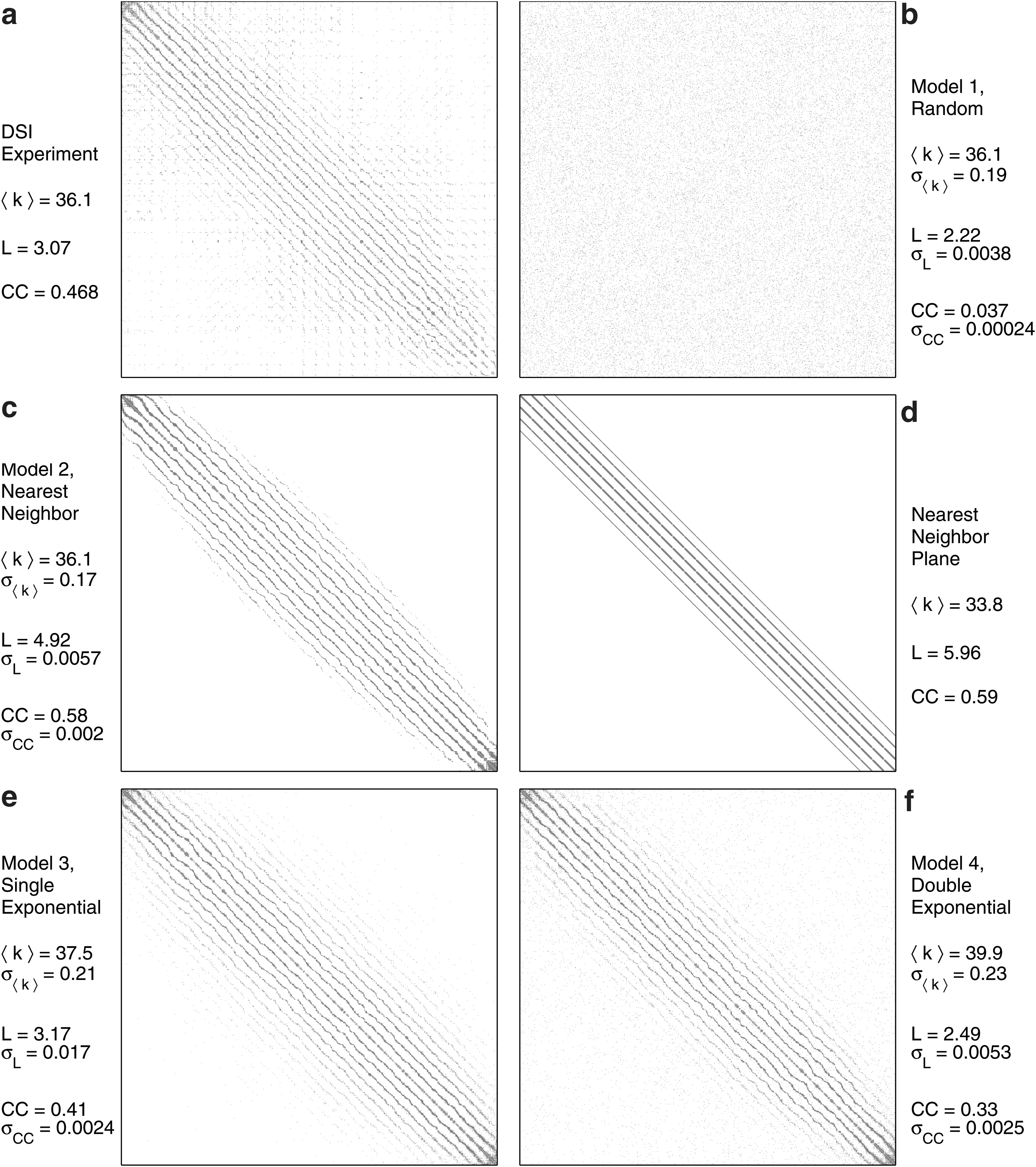
Visual and network-measure comparison of experimental and model networks. Quoted measure values are means and standard deviations of an ensemble of instances of each model, and CMs are example networks drawn from the ensembles with black dots indicating connections.
Geometric indexing allows a number of nonuniform features of the DSI connectivity data to be identified in Figure 2, and Supplementary Figures S2 and S3, with the most obvious being:
(i) The bottom left and top right quarters of the CM in Figure 2b contain the inter-hemispheric connections, with connections between lateral areas toward the edges of the CM and connections between medial areas toward the central diagonal of the CM. The very low density of connections in these quarters away from the diagonal and the presence of connections close to the central diagonal indicate that the connectivity between hemispheres is predominantly between medial areas near their boundary. Hence, corresponding far lateral areas do not usually have direct connections, or such connections are not detected in these data. The widening of the diagonal connectivity stripe at the center of the CM in Figure 2b indicates that the degree and range of connectivity of medial areas is often greater than lateral areas.
(ii) The off-diagonal connections in the CM of Supplementary Figure S3d and the connections not lying on the main diagonal lines of connectivity in the central region of the CM in Supplementary Fig. S3b indicate that there is significant connectivity among the medial areas within and between hemispheres.
Network measures of model and experimental networks
The visual inspections and comparisons described earlier indicate similarities between the model and the experiment. These are now explored further via numerical comparisons. The implications of a local isotropic, homogeneous connectivity architecture in cortical networks are demonstrated and discussed to infer which properties are similar in both the model and the experiment and that should be attributed to additional features of experimental network structure not included in these models.
Constraining network properties of model networks
The following is a list of four network properties proposed by Robinson et al. (2009) to constrain cortical network models; we briefly describe the constraints here, with full details in Robinson et al. (2009). Next, we briefly discuss qualitatively how a local connectivity rule such as that used in the models presented here naturally meets all these criteria, then analyze the network metrics quantitatively with comparison to experimental data.
(i) The networks have high CC. Local connectivity ensures that connections are clustered and triangular motifs are common, resulting in a moderate to high CC. Local connections, as assigned in Model 3, provide a base framework of clustered connections that could be modified through a process of specialization (e.g., Hebbian learning), to increase clustering.
(ii) The networks have a short mean path length L. The canonical 1D regular network has a large path length of O(n). The local connectivity of these models implies they are regular in nature; however, since they are embedded in two dimensions, the path length scales as
(iii) The total number of connections increases in proportion to number of nodes n to keep wiring length to a constant fraction of total brain volume at large n; the total number of connections cannot increase slower than n without the network becoming disconnected. With a local connection rule, each node's connections depend only on surrounding nodes and, hence, are independent of the size of the network. This implies that the total number of connections increases in proportion to n; so, this criterion is satisfied.
(iv) Dynamical reconnection stability. The network should be dynamically stable; therefore, networks should be divisible into, or combinable from, two subnetworks of any relative size without (a) changing their architecture or the strength of more than a small fraction f of the total number of connections, ideally such that f→0 as n→∞ . This lowers the mean connection density
Interrelating clustering coefficient, path length, isotropy, homogeneity, and geometry in model and experimental networks
Quantitative analysis is required to determine the network properties of the models and to identify which features of experimental data can be accounted for by isotropic, homogeneous local connectivity and which cannot. Features that are not accounted for may be associated with anisotropy and/or inhomogeneity which are likely due to regional specificity of different connectivity rules and real cortex geometry that are not included in these models, thus pointing toward directions for future work.
Figure 5 and Table 1 compare CMs and metrics for experimental and model networks to highlight which features of models appear in the experiment. Figure 5a shows the experimental DSI CM and
Experimental and Model Network Measures
Means and standard deviations of experimental DSI (Hagmann et al., 2008) and model
CM, connection matrix; DSI, diffusion spectrum MRI; CC, clustering coefficient.
Random networks, as seen in the example in Figure 5b, are not brain like; however, it is a well-understood standard network model that can be useful for comparison. Here, we set the probability of connection to give an expected mean degree which is equal to that in the DSI network. This random network has a mean path length that is somewhat lower than DSI, L R=2.22 compared with L DSI=3.07, and very low CC, CCR=0.037 compared with CCDSI=0.468; thus, the architecture of the DSI network differs significantly from the random network.
The nearest neighbor CM seen in Figure 5c has a connectivity range r=0.388 that is chosen to produce a mean degree equal to the experiment. This network is much more similar to DSI visually and in terms of CC, CCNN=0.58, than a random model. Both DSI and nearest neighbor network CMs share a similar visual pattern, with both CMs clearly displaying diagonal stripes of short-range connectivity. This implies that both networks have similarities in their architecture. Closer visual inspection of the nearest neighbor CM reveals fewer off-diagonal, longer-range connections than are present in DSI and provides some explanation for the lower path length in DSI (L DSI=3.07), than in the nearest neighbor model (L NN=4.92). The effect of using a spherical geometry compared with a plane geometry can be seen by comparing this spherical nearest neighbor model to the equivalent plane model in Figure 5d, as in Henderson and Robinson (2011). The spherical geometry significantly reduces L as expected, as a plane does not have periodic boundaries, and, hence, longer paths are required to traverse the network. However, CC is not significantly different, as locally both plane and spherical geometry are similar.
The example Model 4 network in Figure 5f has connectivity parameters that were obtained by fitting to the data in Figure 4; Cs =10.1, Cl =0.0222, rs=0.107, and rl =1.05. The double exponential distribution produces a network qualitatively which is similar to the commonly used small world model network that consists of a regular ring lattice with a random distribution of a small fraction of connections (Watts and Strogatz, 1998); that is, a combination of Models 1 and 2 for a 2D spherical geometry. In Model 4, the short-range exponential component of P(r) gives the network properties that are similar to those of a regular ring lattice (Model 2), while the long-range exponential component gives properties which are similar to a random network (Model 1). However, the decay parameter rl is approximately half the diameter of the sphere, leading to about an order of magnitude variation in this contribution to P(r). As rl becomes closer to, or greater than, the physical size of the system, ≈2R, it more closely approximates a random network. Subsequently, the Model 4 network has a lower CC than Model 2 and a slightly higher L than Model 1. However, we note that while Model 4 visually appears most similar to the experimental CM, having both the diagonal structure and more off-diagonal connections than present in Model 3, its network measures deviate more significantly from the data, indicating that the details of individual connections within the distribution, especially for long-range connections, are important.
The connectivity parameters C and r 0 in Model 3 (Fig. 5e) are fitted to the experimental probability of connection data in Figure 4. The fitted values are C=6.53 and r 0=0.129, with the fitted value of r 0 scaled from 7.45 mm as the cortex was scaled to a unit radius sphere as used in the model. The exponential decay in connectivity with distance is steep; Figure 3 shows that while short-range connections make up most of the connections in this network, with 80% of connections less than 35 mm, such short range connections compose only a very small proportion of all theoretically possible connections between pairs of nodes.
The fitted values, C=6.53 and r
0=0.129, produce a network that is very similar (but not identical) to data visually (with a comparable indexing sequence) and in terms of key measures
Figure 6 shows the degree distribution for DSI experiment and Models 3 and 4. Both Models 3 and 4 show Gaussian distributions as would be expected from the Central Limit Theorem. The DSI
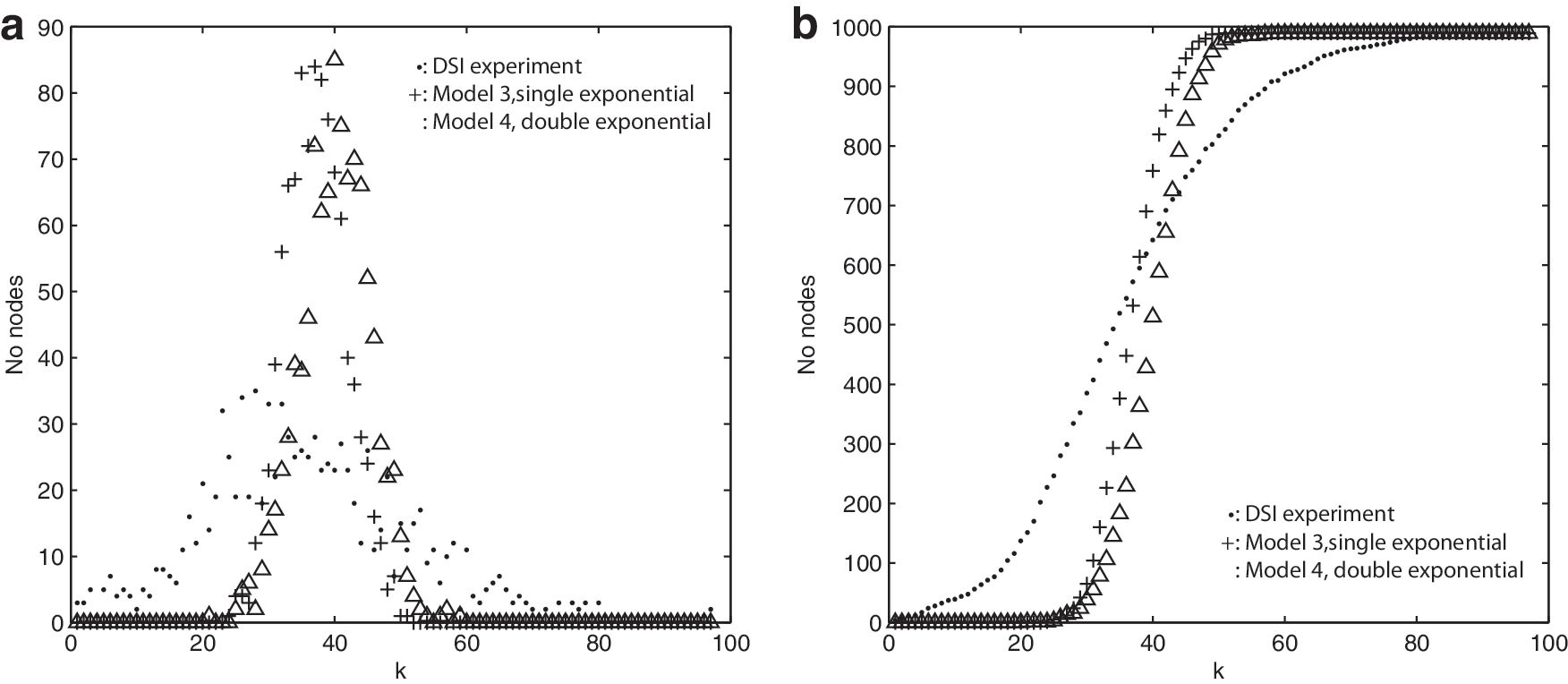
Figure 7 shows L, CC, and
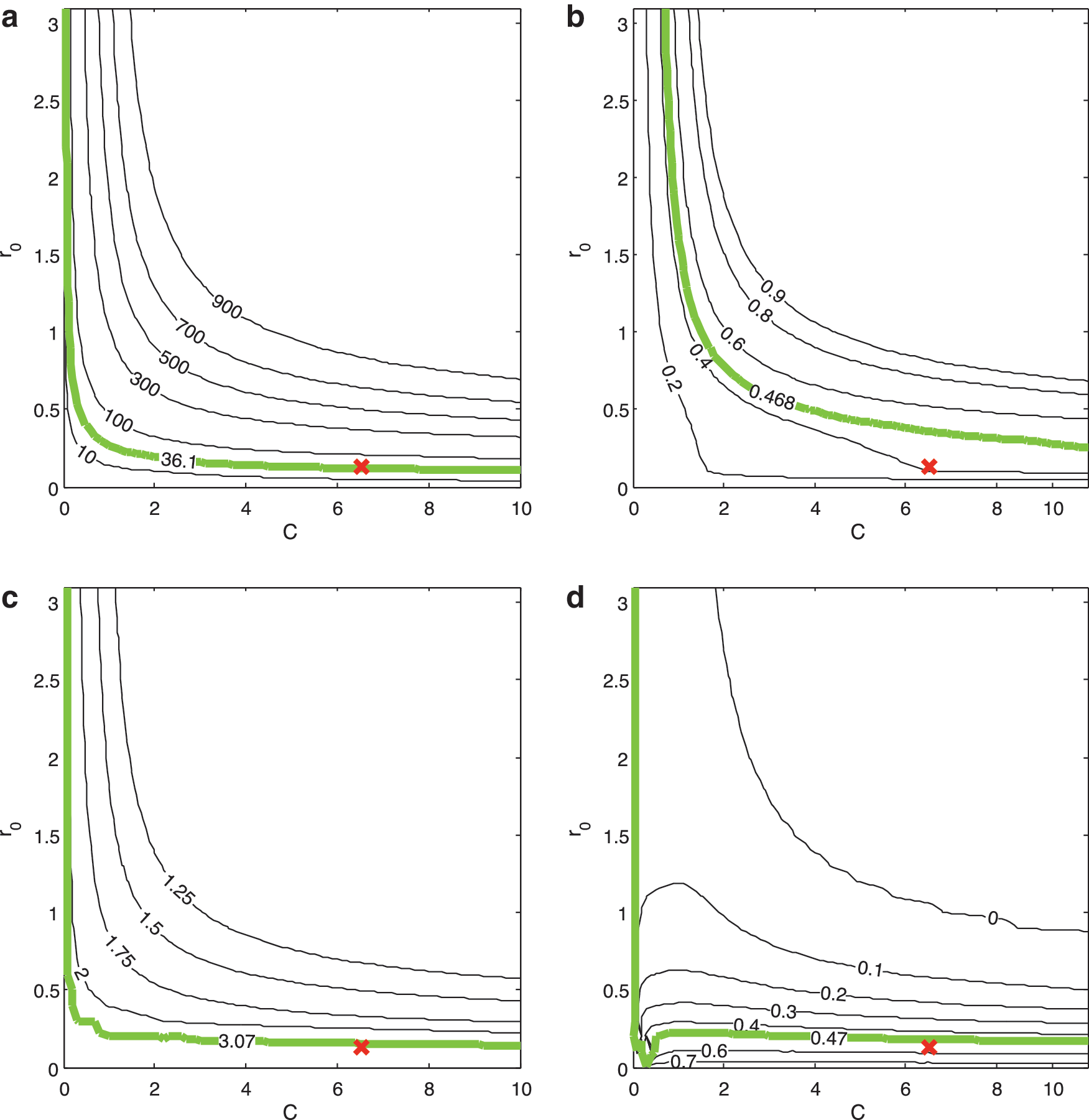
The dependence of key network measures on the single-exponential Model 3 connectivity parameters, C and r
0, in Equation. (1).
These results interrelate isotropic, homogeneous local connectivity with
Interrelating modularity, isotropy, homogeneity, and geometry in model and experimental networks
Cortical networks have been provisionally identified as being modular by various modularization algorithms (Meunier et al., 2009, 2010; Zhou et al., 2006), and by producing CMs that visually appear modular. Often, the identified modules align, at least in part, with groupings of cortical areas that are associated with similar functions. A modular architecture also seems plausible from both information processing and evolutionary perspectives (Robinson et al., 2009); however, the underlying architecture that produces these modules is not well understood. In contrast many anatomical studies have observed that the cortical structure is isotropic and homogeneous to a first approximation (Braitenberg and Schüz, 1998; Kaiser et al., 2009; Schüz and Braitenberg, 2002; Schüz et al., 2006), leading to an apparent paradox.
One common measure of the modularity [as described above; see Eq. (5)] of a particular division of a network into putative modules is obtained by calculating the number of intramodule connections compared with the number that would be expected from a random network with the same degree distribution. If there are more intramodule connections than would be expected from a random network, then it is often asserted that the network has some degree of modularity. The use of a random network as a null hypothesis is an obvious choice, but random networks are not the only type of nonmodular networks and are not necessarily the best choice for comparison. By comparing only with random networks, this is not precisely a measure of discrete modularity, but a measure of how many more connections are present among groups of nodes than are expected for random connectivity. Hence, any concentration of connections increases Q, whether or not they are segmented into discrete modules.
Using the measure of modularity described earlier, we have found that an isotropic, homogeneous locally connected network can yield a high modularity measure, despite its actual uniformity and complete lack of modularity. This can be demonstrated by dividing the network into putative modules grouped spatially, which yields a set of modules with a high degree of intramodule connectivity due to the local connectivity of their composite nodes. Modularity implies structured differences in the connectivity of nodes that result in a unique, segmented division of the network. Despite the potential for a high modularity score, a homogeneously, locally connected network is not modular, because high scoring modular divisions of the network are not unique (Henderson and Robinson, 2011). For example, in the case of a spherical model, we find that the modular divisions can be rotated through any angle without significantly affecting Q. A modified version of Q that reduces the influence of distance effects on modularity has been recently proposed (Expert et al., 2011). It could be used to uncover a less dominant modular structure that is not distance based and may help in identifying inhomogeneity and/or anisotropy in future studies.
In Figure 8b, a Model 3 network is divided into four modules by two perpendicular planes through the origin. Visually, the resulting CM appears to have at least four modules; however, it is isotropically and homogeneously connected and does not contain any modularity. As previously described, naive observation of a CM alone is, thus, not sufficient to determine the properties and structure of a network. The modularity score for this network with four modules is Q=0.53, which indicates significant modularity, despite the network having no modular structure. If the structure of the network were not pre-known, this would not be obvious and could well lead to a false identification of modularity. This further underscores that a high modularity score does not necessarily imply a segmented or unique modular network structure. A high modularity score is possible to be achieved with experimental connectivity data without specifically selecting modules other than by grouping nodes spatially. When divided into four modules as in Figure 8a, the DSI data have a modularity score, Q DSI=0.46, which is similar to that of Model 3.
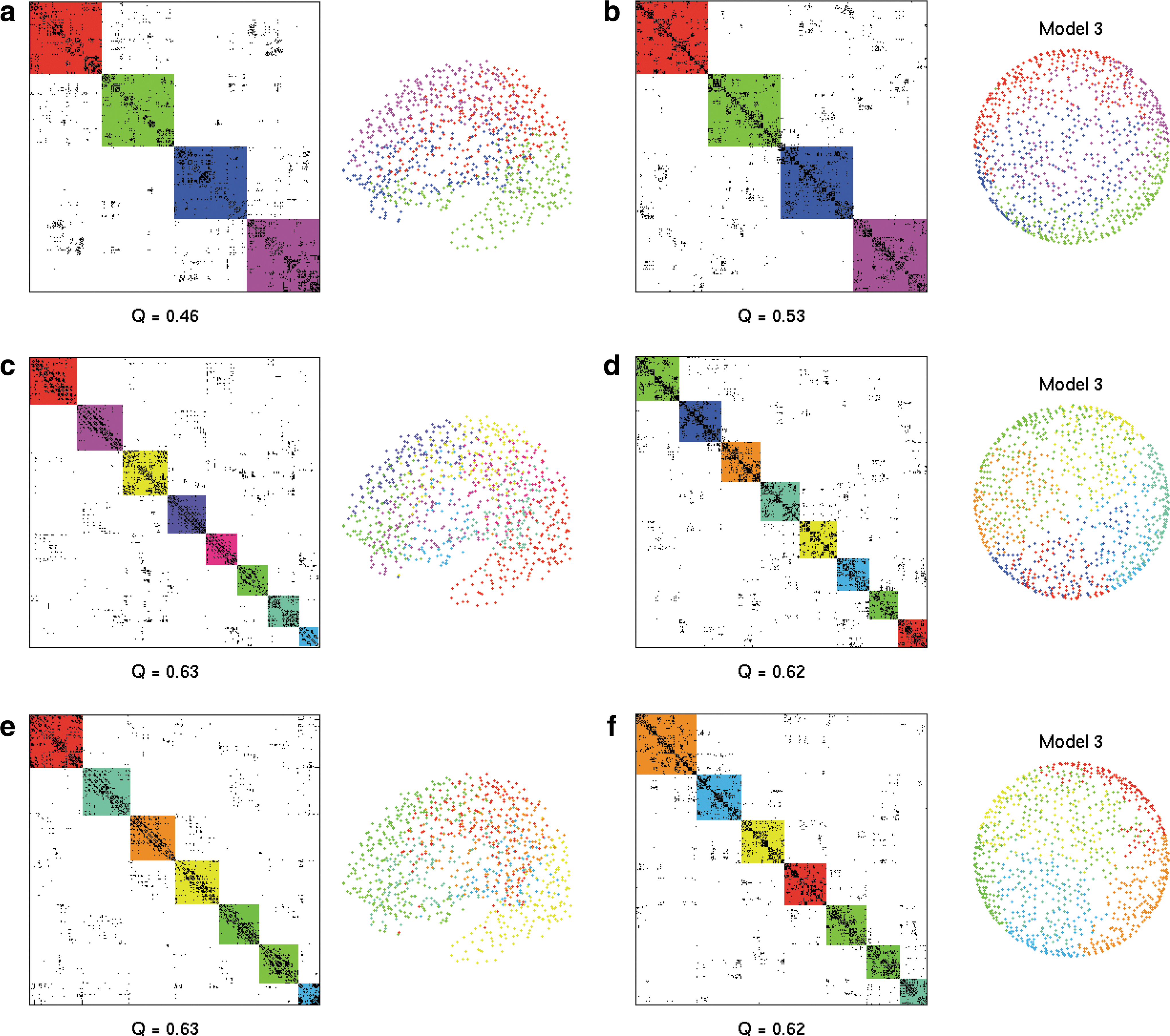
Modular divisions of networks. Left column are CMs, and right column are spatial arrangement of nodes. In both columns, modules are indicated by color.
Two community detection algorithms, Newman's spectral optimization method (Leicht and Newman, 2008) and the Louvain community detection method (Blondel et al., 2008), were applied to the model and DSI networks in Figure 8. For both methods, the model and DSI networks have a very similar modularity score Q DSI=0.63 and Q model3=0.62 and numbers of detected modules. In the DSI data, the nodes contained in each module are grouped spatially and centered around regions of geometrical nonuniformities; for example, temporal lobes and the hemisphere division. Again, the similarity between DSI and model indicates that local connectivity is very important in the modularization of the cortex, and a very segmented, unique modular structure is not required for a network to score highly with a Q modularity measure, as it is enough to have connections that are concentrated at short distances.
We stress that we do not intend to concentrate on any one particular community detection algorithm or measure of modularity. The key concept is that given a division of the cortex into modules, a large portion of intramodule connectivity can be accounted for simply by a homogeneous local connectivity principle without special architecture or connectivity principles. This is a different perspective on cortical architecture from one based on modularity to one based on homogeneity, with perhaps additional weaker modularized connectivity.
In addition to modular structure, hub-like behavior can appear artifactually as follows. Nodes that are positioned spatially near the borders of modules or indexing blocks will have more connections to nodes in their bordering modules or indexing blocks than nodes which are positioned spatially near the center of a module. Hence, such nodes may be interpreted as being connector hubs between modules, despite having the same homogeneous, isotropic connection distribution as all other nodes.
These results interrelate isotropic, homogeneous local connectivity with modularity. Homogeneous, isotropic local connectivity provides an underlying architecture that could potentially be perturbed into a true segmented modular network in the cortex through the addition and/or modification of relatively few connections.
Summary and Conclusions
We have investigated links between the geometric structure of the cortex and its network structure through the development of a geometrically based network model. The network model is based on spherical geometry and isotropic, homogeneous connectivity with an exponentially decaying probability of connection, fitted to experimental data. The main results are as follows:
(i) Node indexing techniques are introduced that can be used to improve CM visualization through a geometric relationship to CM structure which better reveals geometric aspects of connectivity in the CM and enables a better comparison between different CMs.
(ii) The similarity between the homogeneous and isotropic Model 3 network and the experimental DSI data indicates that the overall architecture of experimental cortical networks is also dominated by homogeneity and isotropy. By fitting just two parameters, C and r 0 to DSI experimental data, this model (which has no free parameters) naturally reproduces visually similar CMs, as well as key visualization-independent network measures, CC, L, and Q to that found in experimental DSI data. Thus, these key properties of cortical connectivity have been shown to be primarily direct consequences of, and interrelated by, 2D geometry and isotropic, homogeneous connectivity. Clustering of connections and short path lengths in these models have the same root cause; an underlying 2D geometry in which collections of points have significantly smaller geometrical separation than in 1D (in which model networks are often constructed). Interestingly, this similarity between the model and the experiment includes modularity, Q, despite modularity and isotropy and homogeneity appearing to conflict. This is resolved as follows: Whenever connectivity decreases rapidly with distance, nearby nodes are more strongly connected than would be the case in a random network. This leads to a large positive modularity score, Q, even when the connectivity is entirely isotropic and homogeneous.
(iii) This work begins to differentiate between homogenous and isotropic connections and other types of connections, enabling the identification of which types of connections are responsible for which features of the network. Without first identifying the homogenous, isotropic component as we have done here, the importance of additional specialized connections cannot be assessed. Differences discovered through a comparison of models with experiments lead to further avenues of investigation of connectivity that are not included in these models.
The Model 3 network presented here has a similar, but slightly smaller CC than the experiment. This points toward the presence in the cortex of additional anisotropy and/or inhomogeneity in short-range connections or to effects of more complex cortical geometry (e.g., folding) that increase CC and are not included in the model. This may be a source of unique modular segmentation and a meaningful avenue for further exploring anisotropy, inhomogeneity, modularity, and hierarchy in cortical networks. In addition the Model 4 network containing increased long-range connectivity has network measures deviating from the experiment more significantly from Model 3. This indicates that the long-range connectivity is not drawn from an isotropic and homogeneous distribution as in this model. In future work, finding a suitable theoretical architecture for long-range connectivity to be added to Model 3 that more closely replicates experimental measures may reveal how such longer-range connections in the brain impact network properties.
Isotropic and homogeneous connections can account for most connections in a modular network, with a smaller number of perturbations on this connectivity potentially delineating unique segmented modules, and perhaps contributing a small increase in Q. Small perturbations in connectivity which are designed to delineate module boundaries could be used to construct unique, segmented modules that do not exist with isotropic, homogeneous connectivity and are a topic for future work. This leads to the conclusion that unique, segmented modularity and isotropic, homogeneous connectivity are not as incompatible as they might naively appear.
Consideration of this 2D network model interrelates and reconciles seemingly disparate attempts at modeling the cortex via isotropic homogeneous connectivity as in most mean-field modeling, for example, and the heavy focus on investigations of modularity and hierarchy in cortical network analysis. With further understanding of isotropic, homogeneous connections within the cortex, other connectivity can be distinguished, thereby enabling a more directed study into important features such as modularity and hierarchy. In future work, this or similar models may be used as the basis of a more closely related comparative framework to data than standard random, regular, or small world models. This will enable a specific identification of connections related to more complex inhomogeneous features of the cortex that are not present in these models, such as the effects of cortical folding, specialization of connections, and modular hierarchies. Many of the results and conclusions here also apply to other types of complex networks embedded in 2D geometry.
Footnotes
Acknowledgments
The authors thank Somwrita Sarkar for her useful comments on this article. The Australian Research Council and Westmead Millennium Foundation supported this work.
Author Disclosure Statement
No competing financial interests exist.
References
Supplementary Material
Please find the following supplemental material available below.
For Open Access articles published under a Creative Commons License, all supplemental material carries the same license as the article it is associated with.
For non-Open Access articles published, all supplemental material carries a non-exclusive license, and permission requests for re-use of supplemental material or any part of supplemental material shall be sent directly to the copyright owner as specified in the copyright notice associated with the article.