FATCAT: (An Efficient) Functional And Tractographic Connectivity Analysis Toolbox

Abstract

We present a suite of software tools for facilitating the combination of functional magnetic resonance imaging (FMRI) and diffusion-based tractography from a network-focused point of view. The programs have been designed for investigating functionally derived gray matter networks and related structural white matter networks. The software comprises the Functional and Tractographic Connectivity Analysis Toolbox (FATCAT), now freely distributed with AFNI. This toolbox supports common file formats and has been designed to integrate as easily as possible with existing standard FMRI pipelines and diffusion software, such as AFNI, FSL, and TrackVis. The programs are efficient, run by commandline for facilitating group processing, and produce several visualizable outputs. Here, we present the programs and their underlying methods, and we also provide a test example of resting-state FMRI analysis combined with tractography. Tractography results are compared with existing methods, showing significantly reduced runtime and generally similar connectivity, but with important differences such as more circumscribed tract regions and more physiologically identifiable paths produced between several region-of-interest pairs. Currently, FATCAT uses only diffusion tensor-based tractography (one direction per voxel), but higher-order models will soon be included.

Introduction

Over the past decade, brain connectivity has been studied in several contexts across neuroimaging modalities, using a wide array of tools for both qualitative and quantitative investigation. Functional magnetic resonance imaging (FMRI) (Kwong et al., 1992; Ogawa et al., 1990) has been used successfully to determine the location and extent of distinct brain regions that are organized into networks for performing cognitive functions. In functional connectivity (FC), both task-based (TB-) and resting-state (RS-) FMRI have been used to identify and model interactions within regions forming several gray matter (GM) networks in the brain. RS-FMRI, in particular, permits the examination of several networks from a single scan session (Biswal et al., 1995; Lowe et al., 1998; Xiong et al., 1999). In contrast, diffusion-weighted (DW) imaging methods have enabled the characterization of local white matter (WM) properties based on how anatomical structures affect the random motion of molecules (Basser, 1995; Basser et al., 1994; Le Bihan, 1995). Using this information, tractographic techniques have reproduced several major pathways of WM architecture such as the corpus callosum, cingulate fibers, and corona radiata. (Basser et al., 2000; Catani et al., 2002; Conturo et al., 1999; Hagmann et al., 2003; Mori et al., 1999).

While both modalities have been used to elucidate neural differences between healthy controls and various cases of pathology, anatomical and functional data are often examined in separation, even though functional organization is linked to the anatomical one and vice versa (Simonyan and Ludlow, 2012). More recently, the emphasis on combining these complementary notions of connectivity has grown (Le Bihan and Johansen-Berg, 2012; Sbadbi and Johansen-Berg, 2011; Staempfli et al., 2008), with the goal of providing a better insight into the organization and function of the brain.

Here, we present a suite of software tools for facilitating the combination of FMRI and diffusion-based tractography, called the Functional and Tractographic Connectivity Analysis Toolbox (FATCAT). The point of these tools is to assist in studying both functional networks and their associated WM pathways with the regions of interest (ROIs) forming each network delineated, to the greatest degree possible, by each individual's own data. Succinctly, the tools allow for the delineation of GM ROIs from common FMRI parameters, such as correlation, general linear modeling, or independent component analysis (ICA). An efficient probabilistic tractography algorithm then identifies likely WM regions connecting these GM ROIs, and produces summary properties of these WM regions derived from the diffusion-weighted images.

We discuss the methodology of the tools, highlighting technical and novel aspects. Human data sets are used to demonstrate how the various components of FATCAT can be used for associating functional with structural connectivity measures. This toolbox was designed to integrate as easily as possible with existing standard FMRI and diffusion imaging software such as AFNI, FSL, and TrackVis (Cox, 1996; Smith et al., 2004; Wang et al., 2007). FATCAT is now freely available in the AFNI distribution along with demo data.

The organization of this article is as follows. In the Background section, typical FMRI and diffusion tensor imaging (DTI) processing procedures and parameters are briefly reviewed. In the Design and Methods of FATCAT section, the major components of the toolbox are described, emphasizing both the general purpose of each and technical details of calculation. In the Example Subject Analysis and Results section, examples of FATCAT usage and implementation are given for human data sets; tractographic methods, in particular, are emphasized. Finally, in the Discussion and Conclusions section, the general uses of FATCAT are discussed, along with potential developments for future versions, including higher-order diffusion models for tractography.

Background

We first present a brief background of standard FMRI and DTI methodologies, focusing on the quantities often calculated in each for analysis and comparison. Much more expansive reviews can be found (e.g., Huettel et al., 2009; Kingsley, 2006; Le Bihan and Johansen-Berg, 2012). Then, we show how the features of FATCAT may be used to efficiently combine the complementary measures of FMRI and tractography. In keeping with AFNI's design, FATCAT provides mechanisms of processing with a wide range of application and no single, prescribed pipeline. Users will need to determine how to best combine the tools for the purposes of testing their hypotheses, depending on experimental design, acquired data, overall study goals, and so on. While we present FATCAT for approaches that were considered most common, its design allows for a great deal of flexibility and generality in use.

FMRI and associated quantities

One goal of FMRI studies is to examine functional activation and/or FC across the brain, with the underlying neuronal firing of interest mediated via the blood oxygenation level-dependent (BOLD) response that is actually measured. Traditional TB-FMRI studies identify regions that exhibit a significant BOLD response to a specific stimulus and model their interactions. Alternatively, patterns of BOLD temporal fluctuations across the brain can be studied in the absence of a designated task during RS-FMRI studies. RS-FMRI allows for the concurrent study of several networks based on inter-regional covariance in low-frequency fluctuation (LFF) around the range of 0.01–0.1 Hz. Commonly studied resting-state networks (RSNs) include the sensorimotor, visual, default mode, and executive control networks (Beckmann et al., 2005; Damoiseaux et al., 2006; Raichle et al., 2001; Seeley et al., 2007).

From TB-FMRI, a variety of inter-regional FC measures can be derived such as with structural equation modeling (McIntosh and Gonzalez-Lima, 1994), vector autoregressive modeling (Goebel et al., 2003), structural vector autoregressive analysis (Chen et al., 2011), psychophysiological interactions (Friston et al., 1997), dynamic causal modeling (Friston et al., 2003), and switching linear dynamic system for fMRI (Smith et al., 2011). While the models underlying these varied approaches differ considerably, the result is a measure of connectedness between regions. In RS-FMRI studies, a common approach is to use the standard (Pearson) correlation coefficient as a proxy for connectivity between regions after accounting for a variety of nuisance sources. Another approach uses ICA, which estimates (spatially or temporally) independent maps (Calhoun et al., 2002; Kiviniemi et al., 2003; McKeown et al., 1998). Spatial ICA (SICA) produces several independent component (IC) spatial maps of Z-scores of correspondence to a representative time series for each component. As might be expected, each of the aforementioned methods offers advantages and certain disadvantages in analysis, and even a minor exposition is beyond the scope of this article. Insofar as the toolbox is concerned, these functional measures represent features of a set of GM ROIs that are to be associated with candidate WM regions that can reasonably be connecting them anatomically, and the choice of FMRI analysis is essentially independent of the tractography.

In addition to the tractography tools, several FMRI regional parameters can be estimated with programs within FATCAT, predominantly for RS studies. While not connectivity measures per se, these measures have been found useful in describing resting-state functional connectivity (RSFC). For example, regional homogeneity [ReHo, another term for the previously known Kendall's coefficient of concordance (KCC) (Kendall and Babington Smith, 1939)], can be calculated from the processed time series (Zang et al., 2004). This parameter quantifies the similarity of a time series in groups of neighboring voxels or ROIs. Other descriptors of RSNs in studies of healthy controls and pathological cases include the amplitude of LFFs (ALFF) (Zang et al., 2007), which is the sum of LFF spectral amplitudes of the Fourier-transformed time series; the fractional ALFF (fALFF), in which the ALFF is scaled by the sum of the time series' amplitudes across the full spectrum (Zou et al., 2008); and resting-state functional activity (RSFA), the standard deviation of the LFF-filtered time series (Kannurpatti and Biswal, 2008).

DTI, associated quantities and tractography

As with FMRI, several categories of DW scanning exist, encompassing different levels of structural information, model assumptions, reliability, and power. In all cases, the relative magnitude of diffusion along a given orientation is used to gauge the amount of local structure hindering the journey of hydrogen in water.

DTI utilizes the simplest framework, in which the local diffusion properties are represented by a diffusion tensor (DT), D, having six independent elements. Due to the model assumptions of a positive, semi-definite tensor, D corresponds to the surface of an ellipsoid aligned along the greatest orientation of diffusion in a voxel. At the cost of more DW scans and greater DW magnitude, higher-order models such as high angular resolution diffusion imaging, Q-ball imaging, diffusion spectrum imaging, orientation distribution functions, and others, have the advantage of being able to characterize several dominant directions of diffusion (Anderson, 2005; Özarslan et al., 2006; Tuch, 2004; Tuch et al., 2002; Wedeen et al., 2005). In the current version of FATCAT, only DTI-based tractography (i.e., one main diffusion direction per voxel) is supported, although multi-directional transport is planned for the next release.

In DTI, the number of DW measures along distinct gradients is typically in a range of M=20–30 with a few repetitions of the reference, non-DW measure, and sometimes two to three repetitions of a gradient sequence are performed to increase the signal-to-noise ratio (SNR). From these, several standard parameters of interest may be calculated to characterize important features of the diffusion ellipsoid. The orientation and magnitude of the ellipsoid's semiaxes are, respectively, characterized by the DT's three, mutually orthogonal eigenvectors and the three eigenvalues. Thus, the first eigenvector, e₁ , provides the spatial orientation of the major diffusion direction, whose magnitude is characterized by the first eigenvalue, L1 (by convention, eigenvalues appear in descending order). The average diffusivity in the plane perpendicular to e₁ is given by the radial diffusivity, RD=(L2+L3)/2, the average of the second and third eigenvalues. The relative shape of the ellipsoid is generally quantified by the fractional anisotropy (FA), a normalized standard deviation of the eigenvalues ranging between 0 for isotropy (spherical diffusion) and 1 for maximal anisotropy (elongated diffusion). The mean diffusivity, MD=(L1+L2+L3)/3, relates to the size of the ellipsoid.

In the simplest interpretation, ellipsoids of high FA characterize voxels with major, underlying tract bundles, along which e₁ is aligned. RD may then characterize the relative amounts of cross-structure. Tractography algorithms make use of such associations to estimate the locations of extended structures across many voxels. For deterministic tractography, seed points start in voxels above a threshold FA value and then propagate [using, for example, the local first eigenvector, Euler integration of vector fields or trajectory deflecting schemes (Basser et al., 2000; Conturo et al., 1999; Lazar et al., 2003; Mori et al., 1999; Weinstein et al., 1999; Westin et al., 1999)] until a stop criterion is reached. Tracts passing through selected ROIs are stored, along with their voxel locations. With probabilistic tractography, the variances of FA and e₁ estimates are taken into account, and many iterations of whole brain tractography are run with voxel parameters perturbed at each instance according to estimated parameter uncertainties. The resulting maps show likely locations of WM connecting the target ROIs. In FATCAT, both deterministic and probabilistic tractography utilize the fiber assessment by continuous tracking, including diagonals (FACTID) algorithm, an efficient form of streamline tractography validated in a series of tests on both human data and a standard phantom (Taylor et al., 2012).

Design and Methods of FATCAT

A schematic diagram showing stages for combining FMRI (dark gray boxes) and DW-tractographic (lighter gray boxes) analyses is shown in Figure 1. The functional data may be either TB or RS, with specific steps for processing the latter shown with dashed lines. Dot-dashed lines show alternate side analyses for the DW data. The roles for the main tools in FATCAT are highlighted (bold, blue text), and general steps to be performed with existing software are given as well (italic text). For example, the first set of steps after acquiring either FMRI or DW data typically involves some pipeline of “preprocessing.” This may include motion correction and registration of volumes, spatial smoothing, and despiking (or censoring) of “bad” data points, among other steps.

FIG. 1.

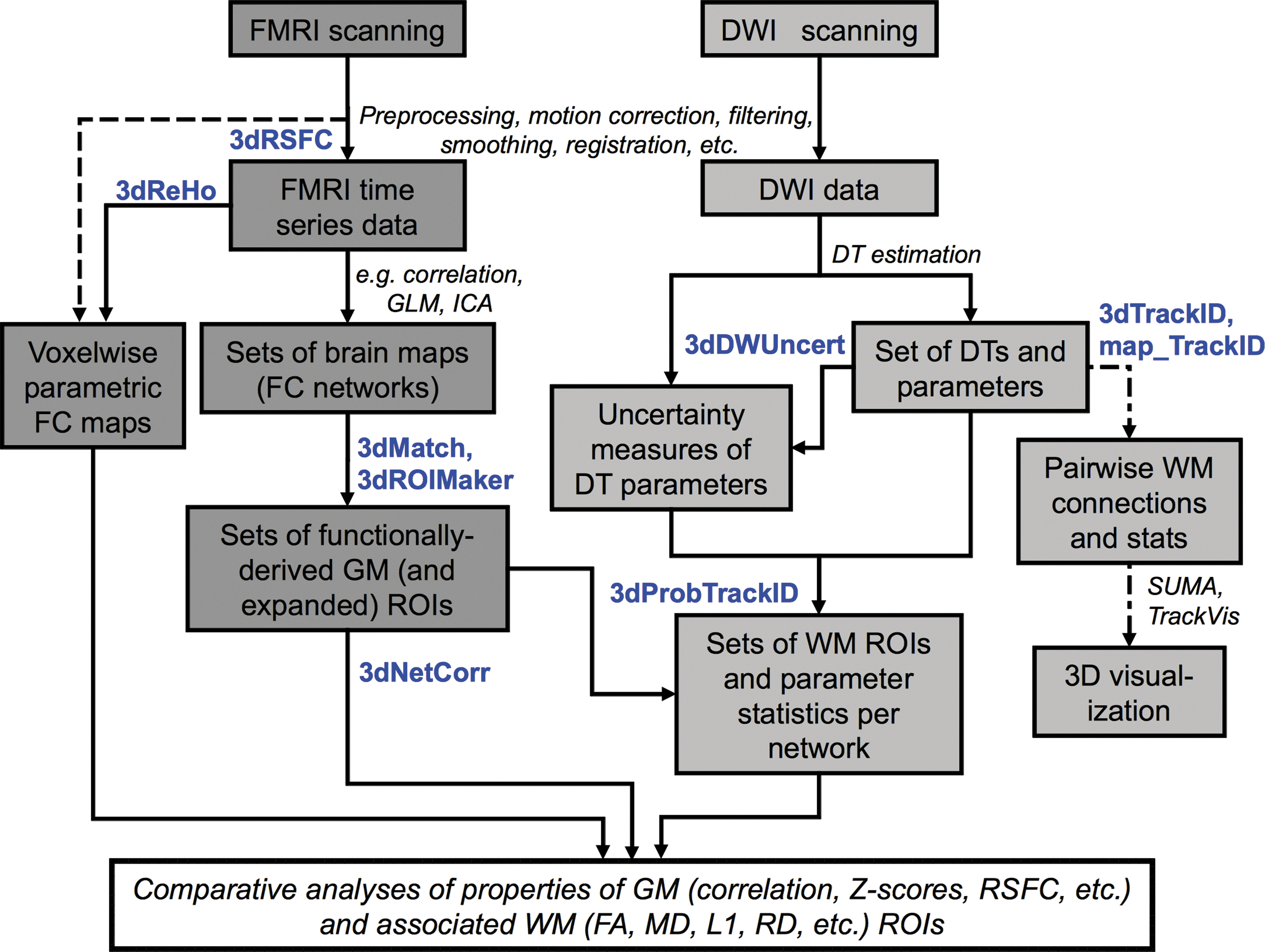
Schematic of a set of stages of combined functional magnetic resonance imaging (FMRI) (dark gray boxes) and diffusion tensor imaging (DTI)-tractography (light gray boxes) analyses, highlighting the possible use of Functional and Tractographic Connectivity Analysis (FATCAT) programs (bold, blue) and showing additional steps in available software (italics).

Functional processing

Standard goals for functional processing include, but are not limited to, localizing regions of activity, quantifying local properties, and measuring connective properties among networks of these ROIs. All of these objectives are realizable for both TB- and RS-FMRI using tools in FATCAT, though we note that several of the calculable ROI-based quantities have typically been used more commonly for the latter studies. In terms of localizing functional ROIs and defining targets for tractography, however, both TB- and RS-FMRI data sets are commensurately useful.

3dRSFC is a program that is used for estimating a variety of common RSFC parameters: ALFF, fALFF, RSFA, and fRSFA (a quantity introduced here, the RSFA scaled by the standard deviation of the pre-LFF filtered time series). Since parameters such as fALFF and fRSFA are drawn from both the LFF and unfiltered series, one should be sure that the spectral features of both are calculated after identical processing. 3dRSFC also combines preprocessing features of AFNI's 3dBandpass (e.g., detrending, regressing, despiking, filtering, and spatial smoothing) with parameter estimation to ensure that both LFF and unfiltered time series have analogous processing for comparisons of spectral amplitude. The outputs of this program are a data set of fully processed LFF time series and associated whole-brain maps of RSFC parameters.

3dMatch takes two sets of volumes and pairs them in a manner that maximizes the match between volume singletons. This may be used to associate and order ICA results from an individual with those of a standard reference set, as ICA results are unordered, in general. For two sets A and B, similarity is weighted toward higher intensity voxels with a match being estimated as the correlation of volumes A′=sign(A)×A² with B′=sign(B)×B². There are options to set ceiling and floor values for the volumes, and one may output Dice coefficients of comparison (Dice, 1945) between masks of thresholded volumes as well.

3dReHo computes ReHo (KCC) on a voxelwise or on a regionwise basis. In the voxelwise case, neighborhoods may be selected around each individual voxel (i.e., neighborhoods of 6, 19, or 27), or may be formed from extended spheroidal and ellipsoidal shapes; the latter may be useful, in particular, in the case of anisotropic voxel dimensions. The ReHo parameter has been used in both TB- and RS-FMRI studies (He et al., 2007; Zang et al., 2004). In addition, the Friedman chi-square of the coefficient is estimated.

3dROIMaker is used to parcellate whole-brain FC maps of statistical measures into distinct GM networks by thresholding and spatial clustering. Individual ROIs are labeled with distinct integers, which can be made uniform across a group by supplying an approximate reference map. ROIs can be thresholded by volume to suppress clusters formed by chance (for example, using levels determined by 3dClustSim in AFNI). In addition, a reference WM image (such as calculated by anatomical image segmentation or by the FA map estimated in the DW processing pipeline, to be discussed next) can be used as a reference to trim away voxels that may have large partial voluming. Thus, the first result of using 3dROIMaker is a labeled map (or set of maps, if sets of volumes are provided) of GM ROIs considered to form a FC network.

The second main output of 3dROIMaker is relevant for complementing the FC study with that of tractography. One would like to be able to find regions of WM that are related to each GM ROI and which provide physical connections between ROI pairs. The (probabilistic) tractography to be used to estimate these pathways is described next, but one basic requirement will be that the “target” ROIs input into the algorithm have some junction with WM voxels in order to search for intersecting fibers. Without such an interface, it is difficult to commence or terminate tracts in regions of GM because the FA there is quite low (i.e., typically below tract propagation thresholds). Previous studies for producing targets have included inserting sizable spheres or uniformly inflating the ROI with the aim of reaching WM, both of which may severely overexpand into WM not associated with the GM. In 3dROIMaker, ROI inflation is also employed; however, the expansion of an ROI is halted wherever it reaches WM-labeled voxels in the reference image, reducing one likely category of errors.

Finally, standard Pearson correlation of mean time series between all pairs of the GM ROIs can be calculated using 3dNetCorr. For each network, a correlation matrix is returned, with the option to also return a matrix of associated Z-scores as well. Such matrices are standard quantities of FC in networks.

DW processing

The goal for this line of processing is to resolve primary diffusion paths through WM, with an eye toward identifying the likely location of WM associated with the functionally defined GM ROIs using DW data. The main mechanism for doing so is probabilistic tractography, which utilizes the uncertainty in the estimated DT ellipsoids and Monte–Carlo simulations of whole-brain tractography to find likely WM voxels associated with individual and pairs of assigned targets (Behrens et al., 2003; Parker et al., 2003). Again, the stages of processing are shown in Figure 1.

Typically, the primary features of preprocessing for DW images is volume registration, the attempted correction for eddy currents and sequence-induced distortions, and the elimination of drop-out or error-dominated slices. Examples of existing software and pipelines for these aspects include TORTOISE, RESTORE, and FSL Diffusion Toolbox (Chang et al., 2005; Pierpaoli et al., 2010; Smith et al., 2004). Real-time motion correction, performed during the acquisition of data, may also be used and offers advantages compared with post-processing corrections as seen in measured changes in ellipsoid parameter distributions, for example (Alhamud et al., 2012; Benner et al., 2011; Kober et al., 2012). After preprocessing, the diffusion ellipsoids and parameters (particularly FA and e₁ for tractography and MD, RD, and L1 for statistical purposes) are easily calculated, with nonlinear fitting methods providing greater accuracy. These are available in most standard analysis packages (e.g., FSL-dtifit and AFNI's 3dDWItoDT were used here).

With tensors estimated, a useful first step in tractographic analysis is utilizing the deterministic method to visualize the data. 3dTrackID estimates tracts across the whole brain and between pairs of ROIs (using AND or OR logic). Tracts are generated using the FACTID algorithm, an improvement of the earlier FACT (Mori et al., 1999). FACTID is a streamline algorithm that propagates tracts through each voxel along the local e₁ orientation, but it also includes a test at voxel edges and corners for continuing along a diagonal trajectory. The inclusion of this simple diagonal test has been shown to reduce sensitivity to noise and coordinate axes biases, without the need for data smoothing and while maintaining efficient propagation (Taylor et al., 2012). Standard options for tract continuation can be selected: FA remaining above a certain threshold (e.g., > 0.2), and the angle between e₁ in successive voxels being below a certain value (e.g., <60°). In addition, instead of an FA criterion, one may use a separately generated WM mask, such from segmentation of an anatomical image, to constrain tract propagation.

Basic statistics of the region though which numerical tracts pass are automatically calculated: mean and standard deviation of FA, MD, RD, and L1, as well as mean length and numbers of tracts. The output tracts can be mapped to other coordinate spaces using map_TrackID, a procedure that can be useful for multisubject comparisons in standard space. Results are visualizable in 2D form, highlighting voxels through which tracts have passed, as well as in 3D projections using TrackVis (Wang et al., 2007) or SUMA (Saad and Reynolds, 2012; Saad et al., 2004).

Due to the nature of MRI scanning, all parameter estimates have noise and errors incorporated into their final values. It is useful, therefore, to quantify confidence intervals of uncertainty, particularly for performing probabilistic tractography. The next subsections describe in detail the technical aspects of these procedures in FATCAT.

Uncertainty estimates with jackknife resampling

In the FACTID algorithm, the main DT parameters of interest are FA and the first eigenvector, as these, respectively, determine the proxy location of WM and the orientation of propagating tracks. In particular, the vector e₁ has two degrees of freedom for varying, so that two confidence intervals are required; its possible motion is accounted for by estimating how far it could reorient along the mutually orthogonal e₂ and e₃ axes. In 3dDWUncert, the uncertainty estimates for FA and e ₁ are calculated using jackknife resampling (Efron, 1982), which is efficient in terms of both scan time and computation. Jackknife resampling works by analyzing subsets of a data set, from which it builds a theoretical pseudo-population (more details below). This method is broadly applicable to existing scan protocols and, importantly, does not require repeated acquisitions as, for example, the related bootstrap methods do.

In order to obtain confidence estimates, Monte–Carlo simulations have been used in conjunction with nonparametric resampling techniques (e.g., Pajevic and Basser, 2003), such as the bootstrap (Davison and Hinkley, 1999; Jones, 2003) and direct variants (Chung et al., 2006; Whitcher et al., 2008). In general, statistical resampling is used to investigate a given parameter of interest θ, by generating a distribution of estimates, θ*_i, from which it is possible to calculate an estimator θ′, as well as confidence intervals, standard errors, and so on. In the case of the jackknife technique, this is done using randomly selected (without replacement) subsets of measures to calculate each θ*_i. Therefore, from a single original data set, Y={y ₁,…,y _M}, a (unordered) jackknife sample is created, Y′={y′₁,…,y′_{M
_J}}, by omitting d values such that M _J=M−d, where d is typically much smaller than M. There are N_Y _′=binom(M, M _J) distinct subsets of variables, and the process is repeated a large number of times with the M _J values randomly selected at each iteration.

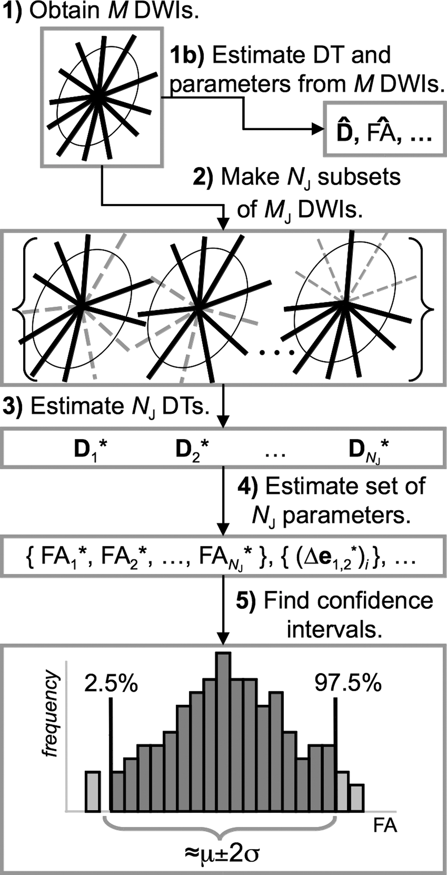
This process is illustrated schematically for diffusion data in Figure 2. In Figure 2-1, M=12 is the number of initial DW measures, shown as gradient directions through an ellipsoid. From these, (Fig. 2-1b) the nonresampled DT estimator, D′, can be calculated, as well as estimators of associated parameters such as FA′, e′₁ , and so on. To perform jackknifing (Fig. 2–2), N _J subsets of M _J=8 measures at a time are randomly selected (bold gradients). Then, the DT of each jackknifed measure is estimated (Fig. 2–3), from which distributions of parameter values of interest are calculated (Fig. 2 –4). In this case, the parameters are the FA and the difference between the jackknifed tensor's first eigenvector and that of the un-jacknifed DT, projected along both the latter's e₂ and e₃ : mathematically, Δe*_1,2=(e′₁−e*₁)·e′₂ and similarly for Δe*_1,3. Finally, the bias and confidence interval of the nonresampled DT estimators are obtained from the jackknifed parameter distributions (Fig. 2 –5).

FIG. 2.

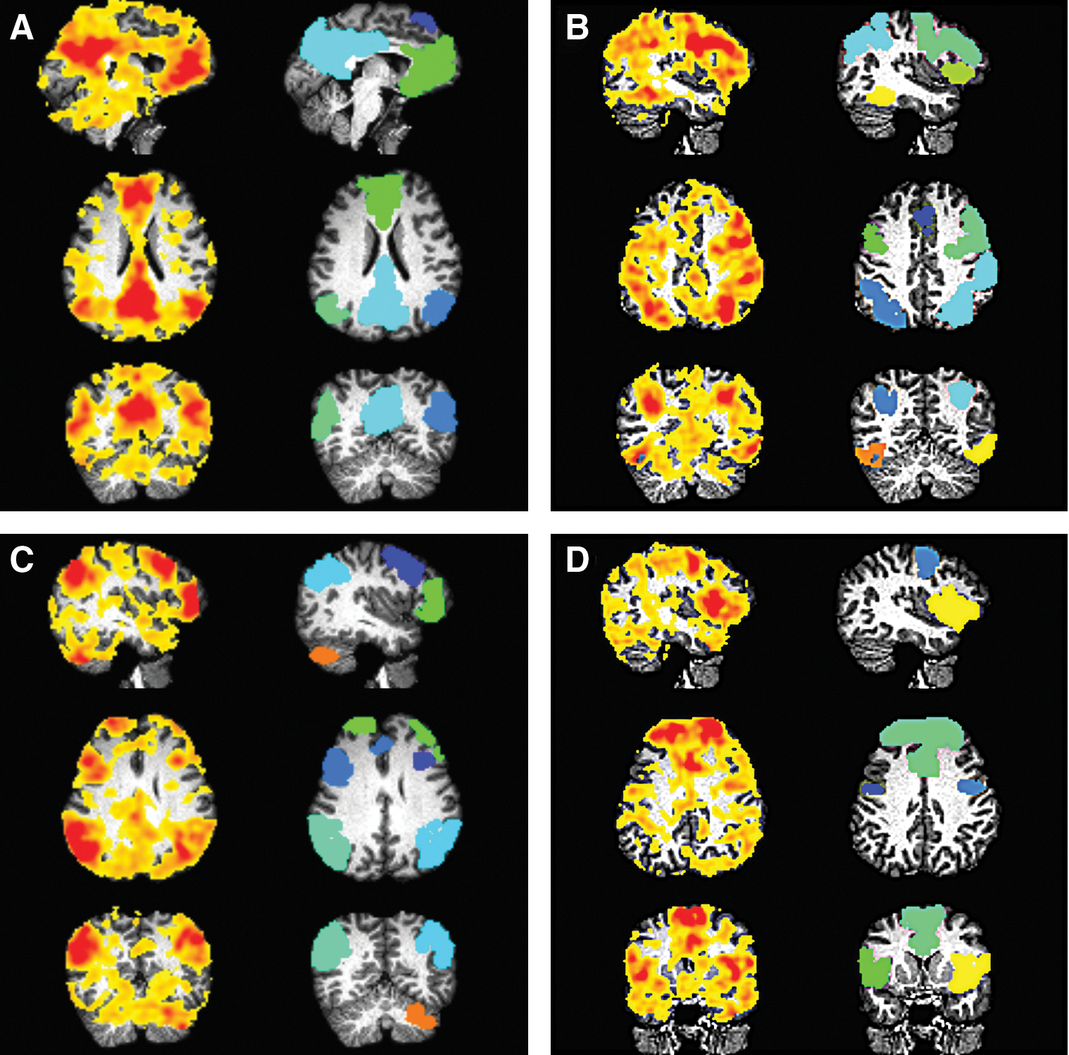
Representation (two dimensional with M=12) of estimating DTI parameter confidence intervals using the jackknife resampling technique. (1) Initial DW measures are obtained, from which (1b) full estimates of the diffusion tensor (DT) and associated parameters are made. For the jackknife process, (2) a random subset of M _J<M measures are selected, from which (3) a sample tensor D* is calculated, as well as (4) its associated parameters. Steps (2–4) are repeated a large number N _J times to create a jackknifed pseudopopulation for each parameter, from which (5) percentile ranges can be found directly from ordering the data set, or from using a Gaussian approximation of the distribution. The latter method is applicable to DTI results and implemented in FATCAT for the sake of efficiency.

FIG. 3.

Four components from independent component analysis (ICA) of RS-FMRI time series overlaid on a T1-weighted anatomical mapped to diffusion-weighted imaging space. Networks were identified with Functional Connectome Project (FCP) group ICs: (A) default mode network (DMN); (B) FCP 20, containing the L-R inferior and superior parietal lobules, middle temporal gyri and the medial and medial frontal gyri; (C) FCP 11, the frontoparietal network; and (D) FCP 17, the cingular gyrus, L-R superior frontal gyri and middle frontal gyri. Z-score maps of each IC are shown (left column of each panel) with images thresholded at Z>0. Also shown are corresponding, inflated regions of interest (ROIs) that are created using 3dROIMaker (colors independent per panel). Initial clusters were thresholded to have >130 voxels, and inflation was stopped at a white matter (WM) skeleton defined to be wherever fractional anisotropy (FA) >0.2.

FIG. 4.

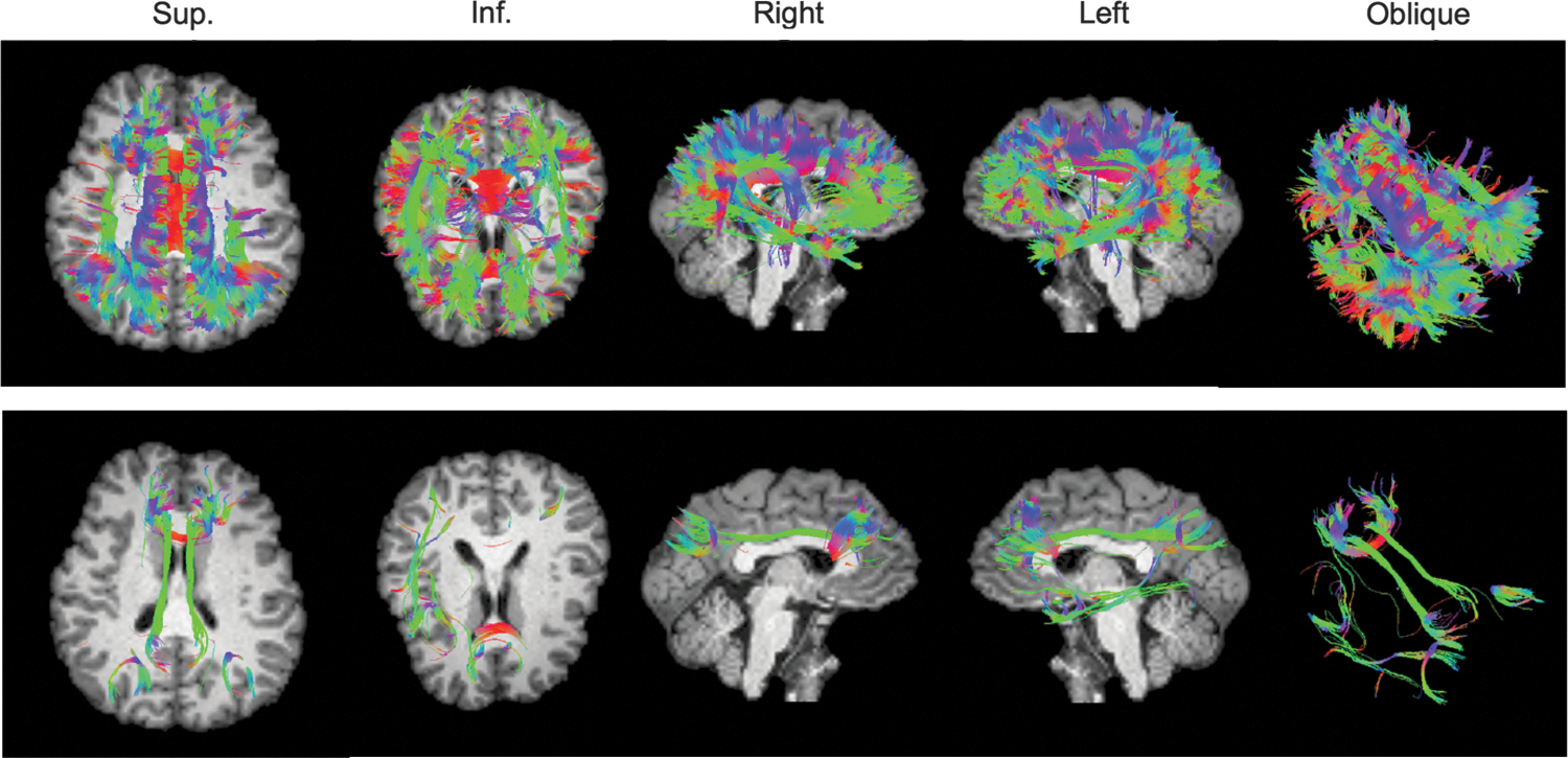
Deterministic tractography results using 3dTrackID with target ROIs shown in Figure 3A. Tracks are displayed using TrackVis, with a T1 image (mapped to DW-native space) as background. In the top row, tracks through any target ROI (OR logic) are shown, and in the bottom row, only tracks passing through pairs of ROIs (pairwise AND logic) are shown.

FIG. 5.

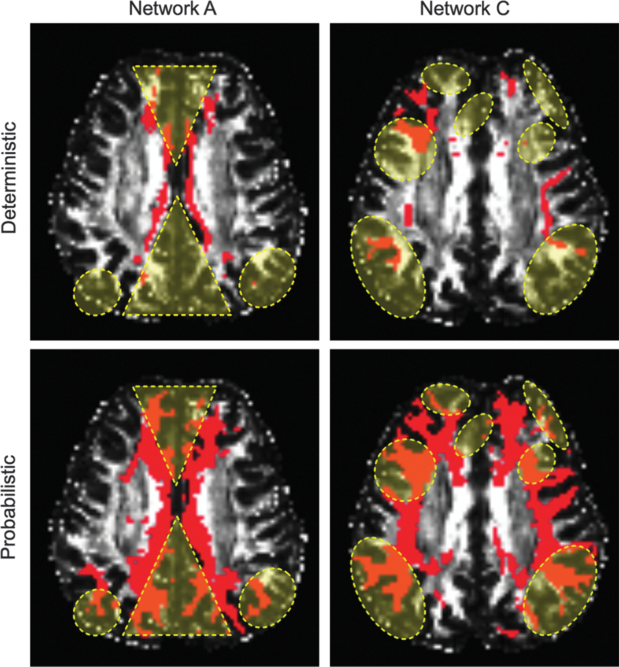
A comparison of WM regions connecting gray matter (GM) ROIs using deterministic (top panels) and probabilistic (bottom panels) tractography for networks A and C (shown in Fig. 3). Approximate locations of GM ROIs are shown with yellow dashes. The deterministic results are a subset of the probabilistic results (here, unthresholded), which shows significantly greater numbers and volumes of WM. Images are in DW-native space.

The confidence intervals are strictly delimited by percentile locations of the distributions or, in the common case of Gaussian distributions, equivalently by known combinations of mean and standard deviation. In FATCAT, the latter, faster approach is used in the uncertainty estimates, as, at SNRs and M values of practical interest, jackknife distributions are well suited to Gaussian approximation. From Monte–Carlo simulations of DW data including Rician noise, a ratio of subsample to sample size of M _J/M≈0.7 generally yielded reasonable estimates of 95% confidence intervals for a large range of SNR and so is used in 3dDWUncert. It should be noted that 3dProbTrackID assumes a minimum amount of uncertainty in the tensor parameters: for e ₁, ∼3° toward either e ₂ or e ₃, and for FA, ∼0.015.

Probabilistic tractography

With the combination of estimated DTI parameters, the uncertainty measures of 3dDWUncert, and the tractography-ready maps of target ROIs from 3dROIMaker, probabilistic tractography can be performed. This is done using a large number of Monte–Carlo iterations of whole-brain (deterministic) tractography estimations using FACTID. With each iteration, FA and e ₁ direction are perturbed at each voxel per the uncertainty estimates, and whole-brain tractography is carried out. Locations of tracts that intersect any pairs of ROIs are recorded. For N _MC iterations with N _seed track seeds per voxel, locations are recorded where more than f _tr N _MC N _seed tracks passed, where f _tr is a user-defined fractional threshold (tracks passing through individual ROIs are recorded separately as well). The set of all voxels connecting a pair of target (expanded GM) ROIs forms a WM ROI.

In several existing algorithms, probabilistic tractography is used to estimate the likelihood that a given target voxel is physically connected to each voxel in the brain, generally as a scaled value of the number of tracts connecting two locations. In FATCAT, however, the tractography results are structured for finding voxels that are likely in the WM connecting given target ROIs; the number of tracts through a voxel is used as an approximate gauge of the likelihood of including the voxel in the WM ROI. This latter interpretation avoids the difficulties of the former in trying to interpret the relative number of numerically reconstructed tracts as a proxy for some physiological “strength of structural connectivity,” as well as the question of how to compare relative strengths between ROIs of different sizes or subjects. Moreover, the WM ROIs themselves are useful outputs, whose structural properties may be probed using DTI quantities therein or mapping the ROIs to anatomical space for studying T1 or proton density values, for example. (It should be noted, though, that the number of tracks between ROIs is still recorded and output as an informational value for the user.)

Statistics of DTI parameters per connective WM ROI are automatically calculated, similar to the 3dTrackID case described earlier (i.e., mean and standard deviation of FA, track number, etc.). For a network of N _ROI GM ROIs, this results in a symmetric N _ROI×N _ROI matrix of values, whose i, jth values are the WM properties connecting ROIs i and j and whose diagonal values are for any tracks through each individual ROI. This matrix is the same size as an FC matrix derived for the same network of GM ROIs.

Example Subject Analysis and Results

In this section, we provide an example case of combining RS-FMRI and DTI-tractography analyses using FATCAT. For a comparison of tractography results, equivalent parts of the FSL-package Diffusion Toolbox software, dtifit, bedpostX, and probtrackX (described next) were also run. We first describe the preprocessing steps for the data sets, the use of ICA with RS-FMRI data to generate networks of ROIs for tractography, and conclude with the tractography results and comparisons.

Preprocessing

The data for this example were collected from a control subject as a part of a larger study, with participants from the university campuses in Taipei. Participants were enrolled after providing written, informed consent. The study was approved by the local ethics committee and conducted in accordance with the Declaration of Helsinki.

Data are shown from one healthy subject (healthy control male, 24 years old). All MR images were carried out on a 3T Trio MR scanner (Siemens) that was equipped with a 32-channel phased-array head coil. A twice-refocused spin-echo echo planar imaging (EPI) sequence was used for diffusion-weighted imaging (DWI) acquisition. Three b=0 and 30 DW images with b=1000 sec/mm² were acquired for each DWI set, with imaging parameters: TR=8800 ms, TE=101 ms, FOV=24×24 cm, BW=1325 Hz/pixel, and parallel acquisition (GRAPPA) with twofold acceleration. A T1-weighted MPRAGE scan was acquired with 256×256×192 voxels (1 mm isotropic resolution). An RS scan was acquired: 200 volumes (TR/TE=2500/30 ms) with FOV=28.4×28.4 cm using 3.4×3.4×3 mm voxels.

Standard preprocessing steps were implemented using AFNI and FSL. RS data were processed following Biswal et al. (2010): First, motion correction with regard to the mean image was performed; time series from WM and cerebrospinal fluid (CSF) were regressed out, as well as size motion parameters (maximum motion in any direction was 0.83 mm); spatial smoothing with a 6-mm full-width at half maximum Gaussian blur was applied; the LFF range for temporal filtering was 0.01–0.1 Hz; mean, linear, and quadratic trends were removed; and the first five time points were removed to avoid pre-steady state signal. For the DWIs, we used FSL-eddy_correct, an affine registration (to the b=0 image) in order to correct for aspects of motion and gradient-induced distortions.

FMRI and DTI analyses

After preprocessing, SICA was performed in native functional space with FSL-melodic (http://fmrib.ox.ac.uk/analysis/research/melodic/), selecting decomposition into 20 ICs, a typical dimensionality in RS-FMRI studies. From the resulting components, four were chosen for tractography analysis because of their wide-brain coverage. The Z-score maps of these components were mapped to DW-native space using an affine transformation via the subject's T1-anatomical image and are shown in Figure 3 (thresholded at Z>0; left column of each panel). Network identifications were made by using 3dMatch in comparison with the 20 group ICs from the multicenter Functional Connectome Project (FCP) study (Biswal et al., 2010). The IC-defined networks are shown in Figure 3 (left columns of each panel), with the following associations (i.e., all ICs here show significant but not identical overlapping with the FCP networks, due, for example, to different splitting of components; see e.g. Groppe et al. [2009]): (Fig. 3A) FCP 6, default mode network (DMN); (Fig. 3B) FCP 20, containing the left and right (L–R) inferior and superior parietal lobules, middle temporal gyri and the medial and medial frontal gyri; (Fig. 3C) FCP 11, the frontoparietal network; and (Fig. 3D) FCP 17, the cingular gyrus, L–R superior frontal gyri and middle frontal gyri.

Each of the Z-score maps were converted to target ROIs for tractography using 3dROIMaker. Clusters were made by first thresholding values at Z>3 and volumes at voxels per cluster >130, and then inflating each ROI by two voxels but stopping expansion at an FA>0.2 WM skeleton. These final target ROIs for tractography are also shown in Figure 3.

Figure 4 shows an example of deterministic tractography results performed in DW-native space with 3dTrackID. The set of tracks running through any of the DMN network ROIs (targets shown in Fig. 3A, second column) is shown using TrackVis. Colors denote local orientation along the tracks. Tracks are shown running along many expected pathways. However, since the deterministic tracts take no account of noise and parameter uncertainty, one can expect that the full, probabilistic tractography results would show more complete pathways among the ROIs. In the top panels of Figure 5, voxels through which tracts passed (for networks A and C in Fig. 3) are shown in red, overlayed on the FA map; in the lower panels of the same figure, WM regions found between GM ROIs using probabilistic tractography (as described next) are shown for the respective networks. Significantly greater extents of WM are included in the latter set.

Two probabilistic tractographic analyses in DW-native space were run for comparison: the existing FSL software approach and the FATCAT method. In the former, first bedpostX was applied to model distributions of relevant parameter values per voxel using a Bayesian Monte–Carlo approach (Behrens et al., 2007); here, only one fiber direction per voxel was modeled (to match the current DTI-based approach of FATCAT). The probabilistic tractography program, probtrackX was then run separately on each network map of target ROIs, using standard stopping criteria and options: FA>0.2, angular deflection <60°, 1 propagation direction per voxel, keeping tracts >15 mm in length, 5000 iterations, integration step size 0.5 mm (FSL default). Using FATCAT, 3dDWUncert was first run for N _J=200 iterations, and example plots of the uncertainty for relevant parameters, in terms of bias and standard deviation estimated using jackknife resampling, are shown in Figure 6. 3dProbTrackID was then run using criteria identical to what was used for probtrackX (except no step size is required) for all four networks simultaneously.

FIG. 6.

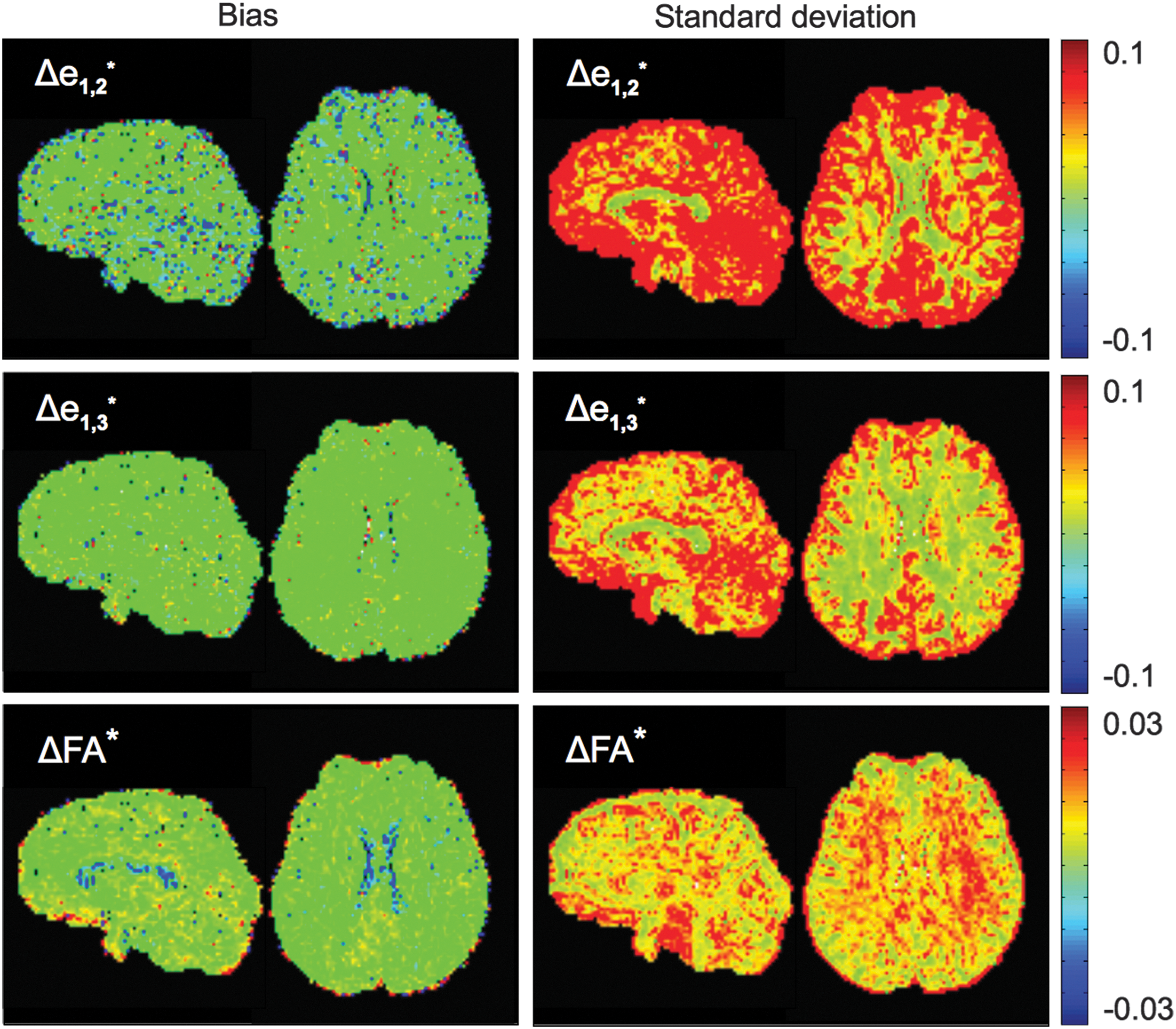
Examples of uncertainty values across brain slices, as estimated with jackknife resampling using 3dDWUncert. Distinct differences in GM and WM are evident, as well as the qualitative difference in first eigenvector uncertainty along the different degrees of freedom.

The results for each program are given in Figure 7. WM ROIs found to connect pairs of target ROIs (orange) are shown in blue (3dProbTrackID) and in purple (probtrackX) for each network. The connectivity patterns produced by each program are broadly similar. Some regions of difference are highlighted with arrows: yellow for tracks appearing in only one set of results, and red for regions in which tracks may have been measured in both results but had very different characteristics (e.g., a filled-in volume vs. filamentary structures). Qualitatively, the 3dProbTrackID WM regions tended to follow more circumscribed paths; for example, in Figure 7A, the anterior–posterior running cingulate bundles are clear, while probtrackX included a much wider volume in the transcallosal region. 3dProbTrackID generally found connections between more ROIs. For example, a transcallosal tract between the posterior parietal lobules was found in Figure 7B, and anterior–posterior subcortical connections (identifiable as the inferior longitudinal fasciculus) in A were found with 3dProbTrackID but not using probtrackX.

FIG. 7.

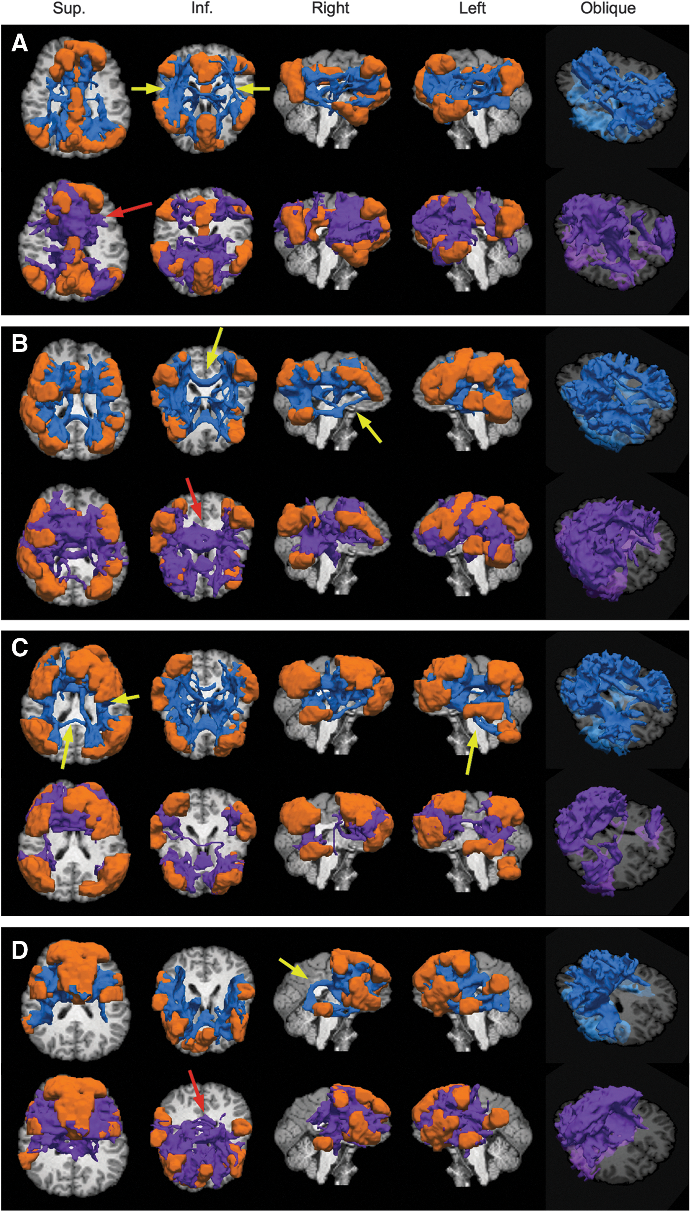
A comparison of probabilistic tractography results for 3dDWUncert+3dProbTrackID (blue) and FSL's bedpostX+probtrackX (purple). Networks of ROIs (orange) were made using ICA of RS-FMRI data, thresholding results at Z=3.0, and then inflating the GM ROIs using 3dROIMaker (each panel A-D represents the same network of ROIs shown the respective panel of Fig. 3; see caption and text for descriptions). Similar tracking options were used for both programs (FA >0.2, angular deflection <60°, 1 propagation direction per voxel, 5000 iterations). Tracking results show broadly similar connectivity, with generally more circumscribed WM track regions found by 3dProbTrackID, which also tended to find connections between more ROIs. Tracking was performed in DW-native space, in which images are shown.

An example of a set of matrices from associated functional and tractographic analyses is shown in Figure 8. In the top row, functional matrices of correlation coefficients and Z-scores (zeroed along the diagonal) are shown, calculated using 3dNetcorr between average time series in GM ROIs that had been calculated using 3dROIMaker for Network A (the DMN; Fig. 3). In the second and third rows, matrices of standard DTI parameters are shown, representing mean values in the track regions connecting GM ROIs as found by 3dProbTrackID. In the bottom row, measures of the number of voxels per WM region and the track count during the probabilistic tractography iterations are given. It should be noted that since not all target regions were found to be connected (to be expected), the structural matrices contain empty cells.

FIG. 8.

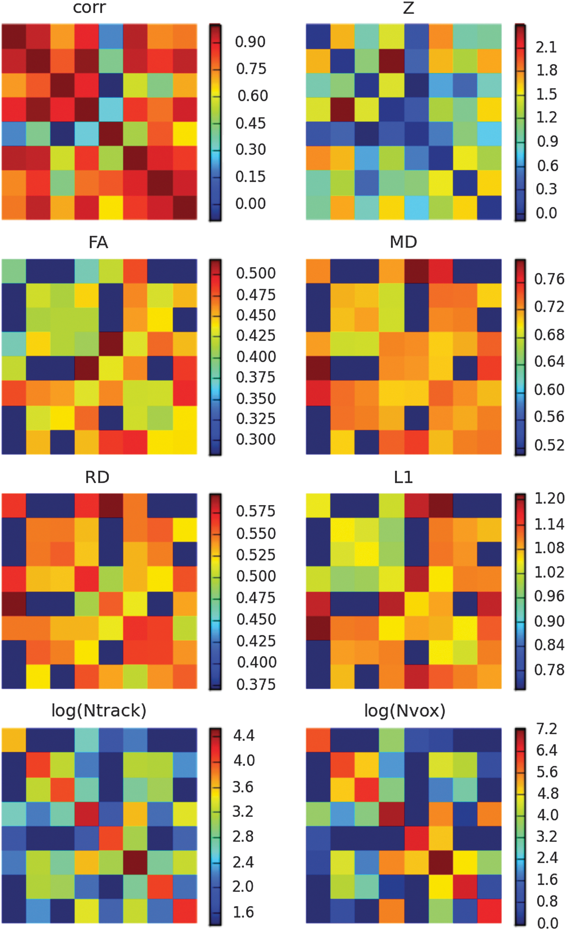
An example set of matrices of functional and structural analyses for network A (the DMN; Fig. 3), as determined using 3dProbTrackID. In the top row are correlation matrices of average time series of GM ROIs in the network (ROI labels have been ignored in this example). In the middle rows, standard DTI parameters are given, representing the mean values in the WM regions connecting the targets. Finally, the number of voxels in the final WM regions and the number of tracts found during the probabilistic tractography are given in the fourth row.

Discussion and Conclusions

We have described a basic set of tools for assisting in two types of MRI analysis: functional MRI and diffusion-based tractography. These methods produce several quantitative measures that can be used in describing complementary features of the brain as highlighted in a recent review (Sbadbi and Johansen-Berg, 2011). Though no single “correct” way for doing so is obvious for lack of ground truths, the software in FATCAT has been designed to assist in this process: simplifying the procedure for calculating several features of both functional and structural connectivity while remaining flexible to types of processing and analysis.

The capabilities and procedures for implementing FMRI and DTI-based tractographic analysis using FATCAT were presented in an example case. Target ROIs for tractography were generated directly from a subject's RS-FMRI data, with 3dROIMaker using anatomical information for determining likely intersections of the functional GM ROIs with nearby WM. Probabilistic tractography results of structural connectivity with 3dDWUncert and 3dProbTrackID were broadly comparable to those of existing FSL programs, in terms of connected GM ROIs and path regions. In the absence of a gold standard, it is difficult to judge which of the two approaches produces more valid results. Qualitatively, 3dProbTrackID results were more spatially circumscribed within WM with more physiologically identifiable paths produced between several ROI pairs.

A striking feature of the FATCAT programs is their relative execution speed. While many programs for probabilistic tractography (including those tested here using FSL) can run for more than a day for uncertainty estimations and tracking within a single network, 3dDWUncert and 3dProbTrackID completed execution in ∼7 and 25 min, respectively, on the same hardware (MacBook Pro, Mac OS X, single processor 2.3 GHz and 4 GB RAM) and for four rather than one network. One of the reasons for this sizable decrease in runtime is the efficiency of the algorithms in each: uncertainty estimations use jackknife resampling of DTI data and utilize the Gaussian interval approximation; the tract propagation algorithm in FACTID is also efficient. Whole-brain tractography using 3dTrackID on a 128×128×70 voxels (2 mm isotropic) dataset took <4 sec on the same machine. Even with more complex diffusion models per voxel such as Qball, the tracking execution speed is not expected to increase significantly. Moreover, testing for connectivity among several networks simultaneously adds very little computational time, which is of great use in multi-component RSN studies.

WM bundles can cross, “kiss” and fan out in complicated structures at spatial scales considerably finer than voxel sizes on the order of millimeters. Such complex patterns are better (though by no means fully) captured with high-order diffusion models that model more than one direction per voxel. At this stage, FATCAT only supports DTI modeling and single direction-per-voxel tractography. Work is currently underway to add multi-direction support using Q-ball modeling in an efficient manner. We are also considering improvements to the methods of defining target ROIs for tractography from functional data. One improvement may consist of using cortical surface models to inform ROI expansion (Greenberg et al., 2012).

As with most neuroimaging analysis tools, further tests of validity will be required, particularly when including higher-order improvements to the methods. Such verification has traditionally been difficult in tractography, given a lack of gold standard tests; even histological data are generally insufficient for examining fine WM structures in the brain. A well-known test phantom model exists for analysis (Fillard et al., 2011; Poupon et al., 2008), and the FACTID tracking algorithm used in FATCAT has been tested on this, as well as on both in vivo and vivo+simulation data sets (Taylor et al., 2012). However, while being quite useful, the phantom cannot match size, scale, and complexity of brain architecture. Similarly, many in vivo tests to date can only be used to verify algorithm behavior through major fiber bundle pathways but not necessarily in finer structures or in crossing/kissing fiber regions. It is possible that neuroanatomical tracing methods (e.g., Dyrby et al., 2007; Schmahmann et al., 2007) may be improved and expanded to study human data sets for greater validation of in vivo tractography. Such evaluations would be useful for continuing to assess tractography algorithms.

In conclusion, FATCAT is a set of publicly available software tools that is used for combining several aspects of functional and tractographic MRI analysis toward a better understanding of brain function. The tools are integrable with many pre- and post-processing pipelines in standard analysis packages. They are also run from terminal command lines, simplifying group processing, and produce easily viewable outputs for guiding analysis. FATCAT programs and demo data are freely available and distributed with the AFNI/SUMA suite (http://afni.nimh.nih.gov), and users are encouraged to use AFNI's message board for support and feedback.

Footnotes

Acknowledgments

The authors would like to thank Ching-Po Lin for the use of test subject data for this work, and Suril Gohel, Xin Di and Bharat Biswal for analysis advice concerning various toolbox components. This research was supported, in part, by the NIMH and NINDS Intramural Research Programs of the NIH and, in part, by the NIH grant R01 AG032088.

Author Disclosure Statement

The authors declare that no competing financial interests exist.

References

Alhamud

, Tisdall

, Hess

, Hasan

, Meintjes

, van der Kouwe

AJW

. 2012. Volumetric Navigators for Real-Time Motion Correction in Diffusion Tensor Imaging. Magn Reson Med, 68:1097–1108.

Anderson

. 2005. Measurement of fiber orientation distributions using high angular resolution diffusion imaging. Magn Reson Med, 54:1194–1206.

Basser

, Mattiello

, LeBihan

. 1994. MR diffusion tensor spectroscopy and imaging. Biophys J, 66:259–267.

Basser

. 1995. Inferring microstructural features and the physiological state of tissues from diffusion-weighted images. NMR Biomed, 8:333–344.

Basser

, Pajevic

, Pierpaoli

, Duda

, Aldroubi

. 2000. In vivo tractography using DT-MRI data. Magn Reson Med, 44:625–632.

Beckmann

, DeLuca

, Devlin

, Smith

. 2005. Investigations into resting-state connectivity using independent component analysis. Philos Trans R Soc Lond B Biol Sci, 360:1001–1013.

Behrens

TEJ

, Woolrich

, Jenkinson

, Johansen-Berg

, Nunes

, Clare

, Mathews

, Brady

, Smith

. 2003. Characterization and propagation of uncertainty in diffusion-weighted MR imaging. Magn Reson Med, 50:1077–1088.

Behrens

TEJ

, Johansen-Berg

, Jbabdi

, Rushworth

MFS

, Woolrich

. 2007. Probabilistic diffusion tractography with multiple fibre orientations: what can we gain? Neuroimage, 34:144–155.

Benner

, van der Kouwe

AJW

, Sorensen

. 2011. Diffusion imaging with prospective motion correction and reacquisition. Magn Reson Med, 66:154–167.

10.

Biswal

, Yetkin

, Haughton

, Hyde

. 1995. Functional connectivity in the motor cortex of resting human brain using echo-planar MRI. Magn Reson Med, 34:537–541.

11.

Biswal

, Mennes

, Zuo

, Gohel

, Kelly

, Smith

, Beckmann

, Adelstein

, Buckner

, Colcombe

, Dogonowski

, Ernst

, Fair

, Hampson

, Hoptman

, Hyde

, Kiviniemi

, Kötter

, Li

, Lin

, Lowe

, Mackay

, Madden

, Madsen

, Margulies

, Mayberg

, McMahon

, Monk

, Mostofsky

, Nagel

, Pekar

, Peltier

, Petersen

, Riedl

, Rombouts

, Rypma

, Schlaggar

, Schmidt

, Seidler

, Siegle

, Sorg

, Teng

, Veijola

, Villringer

, Walter

, Wang

, Weng

, Whitfield-Gabrieli

, Williamson

, Windischberger

, Zang

, Zhang

, Castellanos

, Milham

. 2010. Toward discovery science of human brain function. Proc Natl Acad Sci USA, 107:4734–4739.

12.

Calhoun

, Pekar

, McGinty

, Adali

, Watson

, Pearlson

. 2002. Different activation dynamics in multiple neural systems during simulated driving. Hum Brain Mapp, 16:158–167.

13.

Catani

, Howard

, Pajevic

, Jones

. 2002. Virtual in vivo interactive dissection of white matter fasciculi in the human brain. Neuroimage, 17:77–94.

14.

Chang

, Jones

, Pierpaoli

. 2005. RESTORE: robust estimation of tensors by outlier rejection. Magn Reson Med, 53:1088–1095.

15.

Chen

, Glen

, Saad

, Hamilton

, Thomason

, Gotlib

, Cox

. 2011. Vector autoregression, structural equation modeling, and their synthesis in neuroimaging data analysis. Comput Biol Med, 41:1142–1155.

16.

Chung

, Lu

, Henry

. 2006. Comparison of bootstrap approaches for estimation of uncertainties of DTI parameters. Neuroimage, 33:531–541.

17.

Conturo

, Lori

, Cull

, Akbudak

, Snyder

, Shimony

, McKinstry

, Burton

, Raichle

. 1999. Tracking neuronal fiber pathways in the living human brain. Proc Natl Acad Sci USA, 96:10422–10427.

18.

Cox

. 1996. AFNI: software for analysis and visualization of functional magnetic resonance neuroimages. Comput Biomed Res, 29:162–173.

19.

Damoiseaux

, Rombouts

, Barkhof

, Scheltens

, Stam

, Smith

, Beckmann

. 2006. Consistent resting-state networks across healthy subjects. Proc Natl Acad Sci USA, 103:13848–13853.

20.

Davison

, Hinkley

. 1999. Bootstrap Methods and Their Application. Cambridge, UK: Cambridge University Press.

21.

Dice

. 1945. Measures of the amount of ecologic association between species. Ecology, 26:207–302.

22.

Dyrby

, Sogaard

, Parker

, Alexander

, Lind

, Baare

, Hay-Schmidt

, Eriksen

, Pakkenberg

, Paulson

, Jelsing

. 2007. Validation of in vitro probabilistic tractography. Neuroimage, 37:1267–1277.

23.

Friston

, Buchel

, Fink

, Morris

, Rolls

, Dolan

. 1997. Psychophysiological and modulatory interactions in neuroimaging. Neuroimage, 6:218–229.

24.

Efron

. 1982. The Jackknife, the Bootstrap and Other Resampling Plans. In CBMS-NSF Regional Conference Series in Applied Mathematics Monograph 38, SIAM, Philadelpia.

25.

Fillard

, Descoteaux

, Goh

, Gouttard

, Jeurissen

, Malcolm

, Ramirez-Manzanares

, Reisert

, Sakaie

, Tensaouti

, Yo

, Mangin

J-F

, Poupon

. 2011. Quantitative evaluation of 10 tractography algorithms on a realistic diffusion MR phantom. Neuroimage, 56:220–234.

26.

Friston

, Harrison

, Penny

. 2003. Dynamic causal modelling. Neuroimage, 19:1273–1302.

27.

Goebel

, Roebroeck

, Kim

, Formisano

. 2003. Investigating directed cortical interactions in time-resolved fMRI data using vector autoregressive modeling and Granger causality mapping. Magn Reson Imaging, 21:1251–1261.

28.

Greenberg

, Verstynen

, Chiu

, Yantis

, Schneider

, Behrmann

. 2012. Visuotopic cortical connectivity underlying attention revealed with white-matter tractography. J Neurosci, 32:2773–2782.

29.

Groppe

, Makeig

, Kutasc

. 2009. Identifying reliable independent components via split-half comparisons. Neuroimage, 45:1199–1211.

30.

Hagmann

, Thiran

, Jonasson

, Vandergheynst

, Clarke

, Maeder

, Meuli

. 2003. DTI mapping of human brain connectivity: statistical fibre tracking and virtual dissection. Neuroimage, 19:545–554.

31.

, Wang

, Zang

, Tian

, Zhang

, Li

, Jiang

. 2007. Regional coherence changes in the early stages of Alzheimer's disease: a combined structural and resting-state functional MRI study. Neuroimage, 35:488–500.

32.

Huettel

, Song

, McCarthy

. 2009. Functional Magnetic Resonance Imaging. 2nd. Massachusetts: Sinauer.

33.

Jones

DK.

2003. Determining and visualizing uncertainty in estimates of fiber orientation from diffusion tensor MRI. Magn Reson Med, 49:7–12.

34.

Kannurpatti

, Biswal

. 2008. Detection and scaling of task induced fMRI-BOLD response using resting state fluctuations. Neuroimage, 40:1567–1574.

35.

Kendall

, Babington Smith

. 1939. The problem of m rankings. Ann Math Stat, 10:275–287.

36.

Kingsley

. 2006. Introduction to diffusion tensor imaging mathematics: part I. Tensors, rotations, and eigenvectors. Concepts Magn Reson, 28A:101–122.

37.

Kiviniemi

, Kantola

, Jauhiainen

, Tervonen

. 2004. Comparison of methods for detecting nondeterministic BOLD fluctuation in fMRI. Magn Reson Imaging, 22:197–203.

38.

Kober

, Gruetter

, Krueger

. 2012. Prospective and retrospective motion correction in diffusion magnetic resonance imaging of the human brain. Neuroimage, 59:389–398.

39.

Kwong

, Belliveau

, Chesler

, Goldberg

, Weisskoff

, Poncelet

, Kennedy

, Hoppel

, Cohen

, Turner

. 1992. Dynamic magnetic resonance imaging of human brain activity during primary sensory stimulation. Proc Natl Acad Sci USA, 89:5675–5679.

40.

Lazar

, Weinstein

, Tsuruda

, Hasan

, Arfanakis

, Meyerand

, Badie

, Rowley

, Haughton

, Field

, Alexander

. 2003. White matter tractography using diffusion tensor deflection. Hum Brain Mapp, 18:306–321.

41.

Le Bihan

. 1995. Molecular diffusion, tissue microdynamics and microstructure. NMR Biomed, 8:375–386.

42.

Le Bihan

, Johansen-Berg

. 2012. Diffusion MRI at 25: exploring brain tissue structure and function. Neuroimage, 61:324–341.

43.

Lowe

, Mock

, Sorenson

. 1998. Functional connectivity in single and multislice echoplanar imaging using resting state fluctuations. Neuroimage, 7:119–132.

44.

McIntosh

, Gonzalez-Lima

. 1994. Structural equation modeling and its application to network analysis in functional brain imaging. Hum Brain Mapp, 2:2–22.

45.

McKeown

, Jung

, Makeig

, Brown

, Kindermann

, Lee

, Sejnowski

. 1998. Spatially independent activity patterns in functional MRI data during the stroop color-naming task. Proc Natl Acad Sci USA, 95:803–810.

46.

Mori

, Crain

, Chacko

, van Zijl

. 1999. Three dimensional tracking of axonal projections in the brain by magnetic resonance imaging. Ann Neurol, 45:265–269.

47.

Ogawa

, Lee

, Kay

, Tank

. 1990. Brain magnetic resonance imaging with contrast dependent on blood oxygenation. Proc Natl Acad Sci USA, 87:9868–9872.

48.

Özarslan

, Shepherd

, Vemuri

, Blackband

, Mareci

. 2006. Resolution of complex tissue microarchitecture using the diffusion orientation transform (DOT) Neuroimage, 31:1086–1103.

49.

Pajevic

, Basser

. 2003. Parametric and non-parametric statistical analysis of DT-MRI data. J Magn Reson, 161:1–14.

50.

Parker

, Haroon

, Wheeler-Kingshott

. 2003. A framework for a streamline-based probabilistic index of connectivity (PICo) using a structural interpretation of MRI diffusion measurements. J Magn Reson Imaging, 18:242–254.

51.

Pierpaoli

, Walker

, Irfanoglu

, Barnett

, Basser

, Chang

L-C

, Koay

, Pajevic

, Rohde

, Sarlls

, Wu

. 2010. TORTOISE: An Integrated Software Package for Processing of Diffusion MRI Data. ISMRM 18th Annual Meeting, Stockholm, Sweden, 1597.

52.

Poupon

, Rieul

, Kezele

, Perrin

, Poupon

, Mangin

J-F

. 2008. New diffusion phantoms dedicated to the study and validation of high-angular-resolution diffusion imaging (HARDI) models. Magn Reson Med, 60:1276–1283.

53.

Raichle

, MacLeod

, Snyder

, Powers

, Gusnard

, Shulman

. 2001. A default mode of brain function. Proc Natl Acad Sci USA, 98:676–682.

54.

Saad

, Reynolds

, Argall

, Japee

, Cox

. 2004. SUMA: An Interface for Surface-Based Intra- and Inter-Subject Analysis with AFNI. 2004 IEEE International Symposium on Biomedical Imaging: From Nano to Macro. IEEE Arlington, VA, 1510–1513.

55.

Saad

, Reynolds

. 2012. Suma. Neuroimage, 62:768–773.

56.

Sbadbi

, Johansen-Berg

. 2011. Tractography: where do we go from here? Brain Connect, 1:169–183.

57.

Schmahmann

, Pandya

, Wang

, Dai

, D'Arceuil

, De Crespigny

, Wedeen

. 2007. Association fibre pathways of the brain: parallel observations from diffusion spectrum imaging and autoradiography. Brain, 130:630–653.

58.

Seeley

, Menon

, Schatzberg

, Keller

, Glover

, Kenna

, Reiss

, Greicius

. 2007. Dissociable intrinsic connectivity networks for salience processing and executive control. J Neurosci, 27:2349–2356.

59.

Simonyan

, Ludlow

. 2012. Abnormal structure-function relationship in spasmodic dysphonia. Cereb Cortex, 22:417–425.

60.

Smith

, Jenkinson

, Woolrich

, Beckmann

, Behrens

, Johansen-Berg

, Bannister

, De Luca

, Drobnjak

, Flitney

, Niazy

, Saunders

, Vickers

, Zhang

, De Stefano

, Brady

, Matthews

. 2004. Advances in functional and structural MR image analysis and implementation as FSL. Neuroimage, 23:208–219.

61.

Smith

, Pillai

, Chen

, Horwitz

. 2011. Effective connectivity modeling for fmri: six issues and possible solutions using linear dynamic systems. Front Syst Neurosci, 5:104.

62.

Staempfli

, Reischauer

, Jaermann

, Valavanis

, Kollias

, Boesiger

. 2008. Combining fMRI and DTI: a framework for exploring the limits of fMRI-guided DTI fiber tracking and for verifying DTI-based fiber tractography results. Neuroimage, 39:119–126.

63.

Taylor

, Cho

, Lin

, Biswal

. 2012. Improving DTI tractography by including diagonal tract propagation. PLoS One, 7:e43415.

64.

Tuch

, Reese

, Wiegell

, Makris

, Belliveau

, Wedeen

. 2002. High angular resolution diffusion imaging reveals intravoxel white matter fiber heterogeneity. Magn Reson Med, 48:577–582.

65.

Tuch

. 2004. Q-ball imaging. Magn Reson Med, 52:1358–1372.

66.

Wang

, Benner

, Sorensen

, Wedeen

. 2007. Diffusion toolkit: a software package for diffusion imaging data processing and tractography. Proc Intl Soc Mag Reson Med, 15:3720.

67.

Wedeen

, Hagmann

, Tseng

, Reese

, Weisskoff

. 2005. Mapping complex tissue architecture with diffusion spectrum magnetic resonance imaging. Magn Reson Med, 54:1377–1386.

68.

Weinstein

, Kindlmann

, Lundberg

. 1999. Tensorlines: Advection-Diffusion Based Propagation Through Diffusion Tensor Fields. IEEE Visualization Proceedings, San Francisco, 249–253.

69.

Westin

, Maier

, Khidir

, Everett

, Jolesz

, Kikinis

. 1999. Image processing for diffusion tensor magnetic resonance imaging. Taylor

, Colchester

. Lecture Notes in Computer Science: Medical Image Computing and Computed-Assisted Intervention. Springer-Verlag: Cambridge, 441–452.

70.

Whitcher

, Tuch

, Wisco

, Sorensen

, Wang

. 2008. Using the wild bootstrap to quantify uncertainty in diffusion tensor imaging. Hum Brain Mapp, 29:346–362.

71.

Xiong

, Parsons

, Gao

, Fox

. 1999. Interregional connectivity to primary motor cortex revealed using MRI resting state images. Hum Brain Mapp, 8:151–156.

72.

Zang

, Jiang

, Lu

, He

, Tian

. 2004. Regional homogeneity approach to fMRI data analysis. Neuroimage, 22:394–400.

73.

Zang

, He

, Zhu

, Cao

, Sui

, Liang

, Tian

, Jiang

, Wang

. 2007. Altered baseline brain activity in children with ADHD revealed by resting-state functional MRI. Brain Dev, 29:83–91.

74.

Zou

, Zhu

, Yang

, Zuo

, Long

, Cao

, Wang

, Zang

. 2008. An improved approach to detection of amplitude of low-frequency fluctuation (ALFF) for resting-state fMRI: fractional ALFF. J Neurosci Methods, 172:137–141.