Different Neural Manifestations of Two Slow Frequency Bands in Resting Functional Magnetic Resonance Imaging: A Systemic Survey at Regional,Interregional,and Network Levels

Abstract

Temporal and spectral perspectives are two fundamental facets in deciphering fluctuating signals. In resting state, the dynamics of blood oxygen level-dependent (BOLD) signals recorded by functional magnetic resonance imaging (fMRI) have been proven to be strikingly informative (0.01–0.1 Hz). The distinction between slow-4 (0.027–0.073 Hz) and slow-5 (0.01–0.027 Hz) has been described, but the pertinent data have never been systematically investigated. This study used fMRI to measure spontaneous brain activity and to explore the different spectral characteristics of slow-4 and slow-5 at regional, interregional, and network levels, respectively assessed by regional homogeneity (ReHo) and mean amplitude of low-frequency fluctuation (mALFF), functional connectivity (FC) patterns, and graph theory. Results of paired t-tests supported/replicated recent research dividing low-frequency BOLD fluctuation into slow-4 and slow-5 for ReHo and mALFF. Interregional analyses showed that for brain regions reaching statistical significance, FC strengths at slow-4 were always weaker than those at slow-5. Community detection algorithm was applied to FC data and unveiled two modules sensitive to frequency effects: one comprised sensorimotor structure, and the other encompassed limbic/paralimbic system. Graph theoretical analysis verified that slow-4 and slow-5 differed in local segregation measures. Although the manifestation of frequency differences seemed complicated, the associated brain regions can be grossly categorized into limbic/paralimbic, midline, and sensorimotor systems. Our results suggest that future resting fMRI research addressing the three above systems either from neuropsychiatric or psychological perspectives may consider using spectrum-specific analytical strategies.

Introduction

The human brain is a large and complex network organized by spatial, temporal, and spectral principles. In active mental operation, frequency effects are task sensitive in a topographical manner. For example, electroencephalography (EEG) studies reveal that short-term memory processes are reflected by theta oscillation in the anterior limbic system, whereas long-term memory processes are reflected by upper alpha oscillations in the posterior thalamic system (Klimesch, 1996). Synchronization in gamma spectrum can enable object representation and contribute to the maintenance of information in memory (Bertrand and Tallon-Baudry, 2000). In resting state, neural characteristics also confer physiological and neuropsychological significance. Neuronal oscillation provides supporting context for various functions, including input selection, plasticity, perceptual binding, psychological representation, and learning (Buzsaki and Draguhn, 2004). Frontal alpha asymmetry has long been regarded as a potential indicator of temperament and affective reactivity (Davidson, 1992; Hagemann et al., 1998), and connectivity strengths over several brain regions may have implications in depressive disorder (Fingelkurts et al., 2007; Lee et al., 2011a).

The use of functional magnetic resonance imaging (fMRI) to investigate neural features in resting state is receiving increased attention. In contrast to EEG, the major distribution of blood oxygen level-dependent (BOLD) dynamics and the temporal resolution of fMRI are situated at much lower range. These innate properties render fMRI suitable for investigating slower brain oscillation, which has been proven to be surprisingly informative. An early report by Biswal and associates (1995) revealed that spontaneous low-frequency fluctuations (0.01–0.08 Hz) in fMRI are highly synchronous between the left and right primary motor cortex and also significantly correlated with other brain regions associated with motor function. Subsequent research has similar findings in visual, auditory, and linguistic systems, as well as in the default mode network. Functional interaction in resting state exists not only in humans but also in rats and monkeys (Lu et al., 2012). The slow drift of resting fMRI signals clearly has associated neural origins, although the underlying mechanism of how they interact is still unclear (Lu et al., 2007; Mantini et al., 2007; Scholvinck et al., 2010). Similar to EEG oscillation that is composed of several spectral components, studies have suggested that the low-frequency oscillation of resting fMRI can be further categorized into slow-4 (0.027–0.073 Hz) and slow-5 (0.01–0.027 Hz) (Zuo et al., 2010).

The resting dynamics of BOLD signals at slow-4 and slow-5 reportedly have different amplitudes of low-frequency fluctuation (ALFFs) in basal ganglia (slow-4>slow-5) and medial prefrontal cortex (slow-5>slow-4) (Yu et al., 2014; Zuo et al., 2010). ALFF is the L1 norm of low-frequency BOLD fluctuation, and the preferential ALFF distributions of slow-4 and slow-5 suggested spectrum specificity in certain brain regions. Personalities such as extraversion and neuroticism are correlated with slow-4 and slow-5 ALFF in several cerebral structures related to emotion processing (Wei et al., 2014). Further, abnormal intrinsic brain activity in schizophrenia can be reflected in thalamic and precuneus ALFF at slow-4 and slow-5 (Yu et al., 2014). In addition to ALFF, other regional neural properties are also influenced by BOLD spectrum. Regional homogeneity (ReHo), an index measuring concordance of temporal dynamics, differs between slow-4 and slow-5 at basal ganglia, limbic/paralimbic system, and some cortical areas (Yu et al., 2013). Similar to ALFF, ReHo in schizophrenia shows significant group by frequency interaction (i.e., patient vs. control and slow-4 vs. slow-5) in several brain regions, such as inferior occipital gyrus (IOG) and caudate (Yu et al., 2013).

In addition to regional effects, Liang and colleagues (2012) recently associated slow-4 and slow-5 with different nodal and global topologies at the brain network level. Converging evidence seems to have indicated the existence of two subspectrums in BOLD at 0.01–0.08 Hz, similar to different frequency bands in EEG. Although some reports have demonstrated differences in the frequency effects of slow-4 and slow-5 on neural characteristics, these differences have never been adequately and systemically assessed. This study aimed to elucidate different neural manifestations of slow-4 and slow-5 from local to global scales, namely, regional property, interregional interaction, and network features. Specifically, we explored frequency effects on local neural activities using ReHo and mean ALFF (mALFF; ALFF at each voxel normalized by the mean ALFF of voxels in gray matter [GM]), interregional connection by functional connectivity (FC), as well as on network features using graph theory. The results support the claim that slow-4 and slow-5 BOLD are distinct entities whose different effects are not distributed across the whole brain and are instead limited to several neural systems.

Materials and Methods

Participants

A total of 36 healthy subjects with a mean age of 23.7 years (range 20–29) and gender balanced were enrolled in this fMRI study. Written informed consent as approved by the Local Ethics Committee was obtained from each subject. The experimental stimuli consisted of a white central cross subtending at 1.5° of horizontal and vertical visual angle positioned at the center of the monitor.

MRI data acquisition and preprocessing

All MRI images covered the whole brain and were acquired using a 3.0 Tesla Discovery MR 750 scanner (General Electric, Waukesha, WI) at the Center for Cognition and Brain Disorders, Hangzhou Normal University, China. A high-resolution spoiled gradient echo sagittal image was scanned to facilitate anatomical description and to register functional data to a standard template (repetition time [TR], 8.1 msec; echo time [TE], 3.1 msec; flip angle, 8°; field of view [FOV], 250×250 mm; matrix, 250×250; slice thickness/gap, 1.0/0.0 mm; voxel size, 1×1×1 mm³; number of slices, 176). Sequential T2*-weighted echoplanar images (EPIs) were recorded (TR, 2.0 sec; TE, 30 msec; flip angle, 90°; FOV, 220×220 mm; matrix, 96×96; slice-thickness/gap, 3.2/0.0 mm; voxel size, 2.3×2.3×3.2 mm³; number of slices, 43) to trace dynamic changes in the BOLD effect. Head movement was minimized during scanning using a comfortable external head restraint. A total of 183 whole-brain images were collected for around 6 min. The first three EPI volumes were not analyzed to allow for signal equilibrium.

The Analysis of Functional NeuroImages software package (AFNI) was used to handle the acquired fMRI data. The analytical streamline developed by Jo and associates (2010) was adopted to prepare the resting fMRI images (Jo et al., 2010). Preprocessing steps included despike, realignment (motion corrected), slice-time correction, and spatial normalization to standard stereotaxic space (voxel size 2 mm×2 mm×2 mm; with respect to the Talairach coordinate system). The resulting movement parameters were checked to ensure that motion did not exceed 4 mm in any plane. Two subjects were excluded because of excessive head movements, and 34 participants were included in the subsequent analyses. Several regressors were created and modeled as noises, including six movement parameters, third-order polynomials to fit baseline drift, and tissue-based regressors of white matter (WM) and ventricles (Jo et al., 2010). We constructed the regional WM regressors in two steps. The anatomy images were first segmented by a longitudinal stream in FreeSurfer that partitioned GM, WM, and ventricles (Reuter et al., 2010). WM regressor for each GM voxel was then defined by the average time courses of the surrounding WM voxels within a 15-mm-radius sphere. Notably, WM regressors were local (can differ for each GM voxel), and the other three categories of regressors were global (the same for each GM voxel; movement parameters, detrend polynomials, and two lateral ventricles). After regression, the EPI scans were band passed and then smoothed (Gaussian kernel with full width at half-maximum set at 6 mm) to generate EPI datasets within the frequency range of slow-4 and slow-5. Global signal of the whole brain was not regressed in our analytical model (Saad et al., 2012; Zuo et al., 2013).

ReHo and mALFF

ReHo and mALFF are local properties of the brain. ReHo is a variant of Kendall's coefficient of concordance that is used to measure the similarity of a voxel-time series and its immediate neighboring voxel time-series (Zang et al., 2004). ReHo and FC analyses (see section FC analyses) can be viewed as complementary approaches for investigating the similarities of intra- and interregional BOLD dynamics, respectively. For each voxel of slow-4 and slow-5 images, a cube with edge length of 3 voxels (27 in total; contact at faces, edges, and corners all counted in) was considered in computing its ReHo. ALFF is actually the square root of the power spectrum, and mALFF is normalized ALFF scaled by the mean ALFF value of the GM. Similar to slow-4 and slow-5 ReHo images, we calculated slow-4 and slow-5 mALFF. Paired t-tests were performed to examine the frequency effects of slow-4 and slow-5 on both ReHo and mALFF. False discovery rate (FDR) was used to control multiple comparisons, with the threshold level set at q<0.01.

FC analyses

In contrast to ReHo and mALFF, FC analyses address interregional interactions. Pearson's correlation coefficient was used to represent connectivity strength between two different brain regions. Several steps were taken to accomplish FC analyses using AFNI, including anatomical parcellation, construction of correlation maps, z-transformation, and statistical comparison. The registered fMRI data were segmented into 90 anatomical regions of interest (ROIs) according to JuBrain (Eickhoff et al., 2005). Table 1 shows the abbreviations and corresponding numerical codes. The averaged temporal course for each ROI was retrieved and used as a seed vector to correlate with the BOLD dynamics across the whole brain. Consequently, 90 brain maps of correlation coefficients were each obtained for slow-4 and slow-5. Given that correlation coefficients generally do not conform to student t-distribution, z-transformation was performed using the inverse hyperbolic tangent function (tanh⁻¹). Paired t-tests were performed to examine differences in the frequency effects of slow-4 and slow-5 on FC, and FDR was used to control multiple comparisons with q<0.01. A total of 90 t-statistics maps were computed for each pair of slow-4 and slow-5 volumes based on the ROI seeds.

Table 1.

Parcellation of 90 Brain Regions and Their Abbreviations Based on JuBrain Atlas (Odd Number, Left; Even Number, Right)

No.	Regions	Abbreviation	No.	Regions	Abbreviation
1, 2	Precentral gyrus	PreCG	47, 48	Lingual gyrus	LING
3, 4	Superior frontal gyrus	SFG	49, 50	Superior occipital gyrus	SOG
5, 6	Orbitofrontal cortex (superior)	ORBsup	51, 52	Middle occipital gyrus	MOG
7. 8	Middle frontal gyrus	MFG	53, 54	Inferior occipital gyrus	IOG
9, 10	Orbitofrontal cortex (middle)	ORBmid	55, 56	Fusiform gyrus	FFG
11, 12	Inferior frontal gyrus (opercular)	IFGope	57, 58	Postcentral gyrus	PoCG
13, 14	Inferior frontal gyrus (triangular)	IFGtri	59, 60	Superior parietal lobule	SPL
15, 16	Inferior frontal gyrus (orbital)	IFGori	61, 62	Inferior parietal lobule	IPL
17, 18	Rolandic operculum	ROL	63, 64	Supramarginal gyrus	SMG
19, 20	Supplementary motor area	SMA	65, 66	Angular gyrus	ANG
21, 22	Olfactory cortex	OLF	67, 68	Precuneus	PCUN
23, 24	Superior frontal gyrus (medial)	SFGmed	69, 70	Paracentral lobule	PCL
25, 26	Obitofrontal gyrus (medial)	ORBmed	71, 72	Caudate	CAU
27, 28	Rectus gyrus	REC	73, 74	Putamen	PUT
29, 30	Insula	INS	75, 76	Pallidum	PAL
31, 32	Anterior cingulate gyrus	ACG	77, 78	Thalamus	THA
33, 34	Middle cingulate gyrus	MCG	79, 80	Heschl gyrus	HES
35, 36	Posterior cingulate gyrus	PCG	81, 82	Superior temporal gyrus	STG
37, 38	Hippocampus	HP	83, 84	Temporal pole	TPO
39, 40	Parahippocampal gyrus	PHG	85, 86	Middle temporal gyrus	MTG
41, 42	Amygdala	AMY	87, 88	Temporal pole (medial)	TPOmed
43, 44	Calcarine cortex	CAL	89, 90	Inferior temporal gyrus	ITG
45, 46	Cuneus	CUN

To summarize the 90 t-tests of frequency effects on FC, we simplified the results into a 90×90 matrix. The value of each cell reflected the proportion of voxels in a particular ROI pair that showed significant slow-4 versus 5 differences in FC strengths. Their scores ranged from 0 to 1. For example, the cell (3,5) stored the proportion of voxels in ROI 3 that possessed significant frequency effects based on the correlation maps of seed ROI 5. The resultant summary matrix was symmetrized by averaging the raw matrix and its transposed version. We then applied 30%, 40%, and 50% cutoff values to binarize the matrix. The “50% binary map” illustrated the ROI pairs with no less than 50% of their content that demonstrated significant spectral effects on the FC strengths. Similar procedures were applied for 30% and 40% cutoffs.

The community structures showing the frequency effects of FC were investigated by the algorithm Order Statistics Local Optimization Method (OSLOM, 2nd version [OSLOM2]). A community can be described as a cluster of densely interconnected nodes that are sparsely connected with the rest of the network. OSLOM2 is based on a local fitness function that optimizes the statistical significance of a subgraph compared with the random fluctuation of a global null model (Lancichinetti et al., 2011). OSLOM2 enables the detection of hierarchical and overlapping communities and naturally provides a statistical p-value (OSLOM2 reports the p-value that the program stops so that the true one can be much lower). The performance of OSLOM2 is comparable to the best existing algorithms in several artificial benchmark networks (Lancichinetti et al., 2011). It is noteworthy that our community detection analysis aimed to summarize the brain regions showing differences in FC, not the differences in the modular structures of slow-4 and slow-5 FC maps, which is of theoretical importance but not covered by this study. As to the latter, even though slow-4 and slow-5 FC maps showed some variability in modular organization at several brain regions, they did not require FC differences as premise. Further, since analytic results of resting fMRI researches, including this study, have largely shown symmetrical pattern in the healthy brain, symmetrization procedure was taken before community detection. It is of interest to examine in the future whether there is lateralization in some network features of the brain.

Graph theoretical analysis

Graph theory analysis was performed using the brain connectivity toolbox to examine the differences in FC network features between slow-4 and slow-5. In detail, we band-pass-filtered the data (0.01–0.027 and 0.027–0.073 Hz) and averaged the temporal dynamics of EPI images for each of the 90 ROIs according to the partition of JuBrain atlas as described in the section FC analyses. Pearson's correlation was performed to construct two adjacent matrices for slow-4 and slow-5 for each subject. The sign of the correlations in the connectivity matrices was ignored. Our graph theory analysis was performed on each of the subjects separately for each sparsity value (defined below) and for each of the two frequency bands. The indices of network integration, segregation, nodal centrality, and modularity were compared by paired t-tests, including characteristic path length, global efficiency, clustering coefficient, transitivity, local efficiency, betweenness centrality, and Newman's modularity (Leicht and Newman, 2008).

A fully connected binary network generally does not reveal eye-catching structures. To unveil underlying architecture, the common practice is to threshold a network, thereby creating a sparser matrix as the starting analytical step. Considering that the choice of a specific threshold can be arbitrary, we explored network properties across a series of percentage cutoffs (0–91%, with 1% step) to generate sparsity and to test for consistency of results. Thus, 92 matrices were generated by removing the sub-cutoff connections relative to the total possible number of connections in the network (Achard and Bullmore, 2007). For example, a network thresholded at 70% contained only the highest 30% of correlation values in the matrix. The preserved connections were set to 1, and the deleted connections were set to 0. The seven graph indices listed above were calculated for each of the 92 binary maps. Paired t-tests were used to examine the frequency effects of slow-4 and slow-5 on network properties through 0–91% cutoffs. Except for centrality (which is estimated for each ROI instead of the whole network), the statistical threshold was set at p<0.00054 to correct for multiple comparisons (0.05/92; 92 cutoffs by percentage).

Regarding betweenness centrality, we arbitrarily set the threshold at 0.0001. Given that the neighboring adjacency matrices (e.g., three matrices from 45%, 46%, and 47% cutoffs) shared similar structures and were thus not independent, complete Bonferroni correction of 0.00054/90 (90 is the total ROI number) was too harsh. Nevertheless, we posed another constraint of the consecutive number of significant pairs of “ROI and percent cutoff” being greater than 3. For example, if the betweenness centrality indices of ROI 20 reached p-value of 0.00054 at 45%, 46%, 47%, and 48% cutoffs of FC matrices, ROI 20 was regarded as significantly showing frequency effect. If they reached statistical significance at 45%, 50%, 52%, and 60% cutoffs of FC matrices, betweenness centrality of ROI 20 was not regarded as spectrum sensitive even though there were also 4 cutoffs reaching threshold. This extra constraint may reduce the possibility of spurious positive findings.

Results

Frequency effects on ReHo

A roughly symmetrical pattern was noticed to reflect different frequency effects on ReHo. Compared with slow-5, slow-4 ReHo was significantly and bilaterally enhanced in three major clusters: first, superior orbitofrontal cortex, rectus gyrus, and anterior cingulate gyrus; second, inferior temporal gyrus, fusiform gyrus, and hippocampus; and last, subcortical structures such as ventrolateral thalamus, pallidum (PAL), and caudate head. Conversely, slow-4 ReHo was significantly attenuated in bilateral inferior frontal gyrus, insula, and mediodorsal thalamus and in some midline structures, such as medial superior frontal gyrus, supplementary motor area, cuneus, precuneus, and posterior cingulate gyrus (Fig. 1 and Table 2).

FIG. 1.

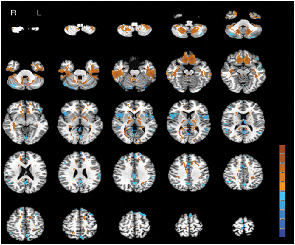
Statistical maps of ReHo analysis. z-Scores of “slow-4 minus slow-5” contrasts are superimposed on a T1 structural image in axial sections from z=−54 mm to z=66 mm, with an interslice gap of 5 mm and FDR q<0.01. The display orientation is in radiological convention (i.e., left is right). The hot color indicates slow-4>slow-5 (maximum=7.23), and blue indicates slow-4<slow-5 (minimum=−5.99). The color bar situated at the right-lower corner represents z-values ranging from −7.23 to 7.23. FDR, false discovery rate; ReHo, regional homogeneity. Color images available online at www.liebertpub.com/brain

Table 2.

Brain Regions Showing Significant Slow-4 Versus Slow-5 Differences in Regional Homogeneity

Brain area (Brodmann area, side)	Stereotaxic coordinates			Voxel size
	Slow-4>slow-5
ACC (24, L)	9	13	34	31
SFG (6/8, L)	13	−11	42	223
SFG (6/8, R)	−19	−15	36	110
PreCG (6, L)	31	1	28	78
PCL (6, R)	−13	15	50	56
PCG (29/30, L)	9	43	16	36
PCG (29/30, R)	−11	39	16	277
PoCG (7, L)	23	37	42	108
PoCG (7, R)	−27	35	38	42
SPL (7, L)	21	55	30	42
SPL (7, R)	−21	53	48	22
MOG (17, L)	17	79	12	42
ITG/FFG (20, L)	53	31	−22	1770
HP (L)	33	11	−10	120
ITG/FFG/HP/CB (20/36, R)	−39	31	−28	2868
ORBsup/REC/ACG (11/24/32, L&R)	11	−29	−16	1878
TPOmed (38, L)	17	−7	−34	30
TPOmed (38, R)	−23	−11	−36	85
CAU head (L)	17	−17	18	55
CAU head (R)	−21	−19	18	78
THA^a/PAL (L)	13	9	2	301
THA^a/PAL (R)	−21	15	2	234
	Slow-5>slow-4
SMA (6, L)	5	−17	58	66
SFGmed (9, L)	3	−45	30	60
MCG (23, L&R)	−1	23	32	107
SFG (9, L)	17	−55	32	20
SFG (8, R)	−11	−39	48	26
MFG (8, L)	33	−19	52	139
IFG/INS (44/13, L)	49	−1	8	216
IFG/INS (44/13, R)	−55	−11	8	385
IFG (47, L)	41	−31	−6	55
PCL (4, L&R)	1	27	68	107
PCUN/CUN/PCG (23/30, L&R)	−1	53	18	704
IPL (40, L)	57	31	24	54
IPL (40, R)	−45	51	42	62
STG (22, L)	45	57	16	25
STG (22, R)	−53	45	12	102
THA^b (L&R)	1	17	12	120

Multiple comparison correction by false discovery rate with q<0.01.

RAI coordinate: negative for right, posterior, and inferior.

The listed coordinates represent peak statistics.

Ventrolateral thalamus.

Mediodorsal thalamus.

RAI, right-anterior-inferior.

Frequency effects on mALFF

Similar to ReHo, bilateral thalamus and caudate head were associated with higher mALFF for slow-4 compared with slow-5 (Table 3). When a less stringent statistical criterion of q<0.05 was selected, ventromedial prefrontal, inferior frontal, and cuneus/precuneus had lower mALFF in slow-4 compared with slow-5. By contrast, slow-4 mALFF was greater than slow-5 mALFF in inferior temporal regions. Thus, the directionality of ReHo and mALFF was not always the same, as shown in Figure 2. Given that the thalamus was the hotspot of different frequency effects in both ReHo and mALFF, the results of thalamus are summarized and illustrated in Figure 3 for better appreciation.

FIG. 2.

Statistical maps of mALFF analysis. z-Scores of “slow-4 minus slow-5” contrasts are superimposed on a T1 structural image in axial sections from z=−54 mm to z=66 mm, with a between-slice gap of 5 mm and FDR q<0.05. The hot color indicates slow-4>slow-5 (maximum=9.44), and blue indicates slow-4<slow-5 (minimum=−6.58). The color bar situated at the right-lower corner represents values ranging from −9.44 to 9.44. mALFF, mean amplitude of low-frequency fluctuation. Color images available online at www.liebertpub.com/brain

FIG. 3.

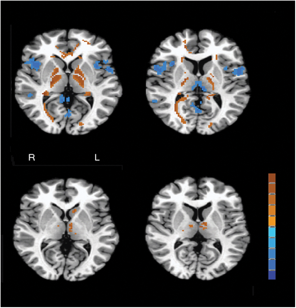
ReHo and mALFF results at subcortical structures. Upper row: axial sections of ReHo results at z=4 mm show slow-4>slow-5 in globus pallidus and ventrolateral thalamus (left subplot, hot color), and those at z=13 mm show slow-4<slow-5 in mediodorsal thalamus (right subplot, blue). Lower row: axial sections of mALFF results at z=4 mm show slow-4>slow-5 in left caudate (left subplot), and those at z=8 mm show slow-4>slow-5 in bilateral thalamus (right subplot). The color bar represents z-scores ranging from −9.44 to 9.44, with hot and blue colors indicating positive and negative values, respectively. Color images available online at www.liebertpub.com/brain

Table 3.

The Brain Regions Showing Significant Slow-4 Versus Slow-5 Differences in Mean Amplitude of Low-Frequency Fluctuation

Brain area (Brodmann area, side)	Stereotaxic coordinates			Voxel size
	Slow-4>slow-5
PoCG (3, L)	27	33	42	31
CAU (L)^a	11	−13	4	28
THA (R)	−11	9	12	48
THA (L)	7	7	8	126
	Slow-5>slow-4
PCG (30, L)	1	49	20	21

Multiple comparison correction by false discovery rate with q<0.01.

RAI coordinate: negative for right, posterior, and inferior.

The listed coordinates represent peak statistics.

Right caudate is significant when q<0.025.

Frequency effects on FC strengths

We computed 90 statistical parametric maps depicting different frequency effects on connectivity strength based on the 90 ROIs defined by JuBrain atlas. Without exception, regarding the paired t-tests of the connectivity strengths with q<0.01, higher frequency components (from the time series at slow-4 range) always showed weaker connectivity strengths than the lower frequency counterparts (from the time series at slow-5 range). The complicated FC results were verified by several analytical steps. First, a summary matrix was constructed, with the cell content equal to the proportion of voxels showing significant frequency effects (Fig. 4). Second, three different thresholds were applied, that is, 30%, 40%, and 50% (Fig. 5). The three binary maps were imported to OSLOM2 algorithm for community detection, and the OSLOM2 results consistently discovered two modules across the three different cutoffs (Fig. 5). No hierarchical structure and only minimal overlapping were detected. 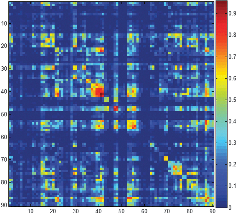The community structures were demonstrated by Pajek software (http://vlado.fmf.uni-lj.si/pub/networks/pajek/) (Fig. 6). For the two modules discovered at 50% threshold, we used AFNI to present their distribution with different colors (Fig. 7). The first cluster comprised precentral gyrus, Rolandic operculum, inferior frontal gyrus, insula, supplementary motor area, middle cingulate gyrus, Heschl gyrus (HES), supramarginal gyrus, superior and inferior temporal gyrus, and basal ganglia. The second cluster included olfactory cortex, medial temporal pole (TPO), hippocampus, parahippocampus, amygdala, fusiform gyrus, precuneus, and thalamus.

FIG. 4.

The matrix is 90×90 and has values ranging from 0 to 1. Each cell stores the proportion of voxels in an ROI (or ROI pairs) that presented statistically significant differences in terms of connectivity strengths between slow-4 and slow-5. This matrix is a summary of 90 ROIs based statistical parametric maps of functional connectivity analyses, corrected by FDR q<0.01. The color bar is located at the right-hand side. Note: the matrix has been symmetrized. ROI, region of interest. Color images available online at www.liebertpub.com/brain

FIG. 5.

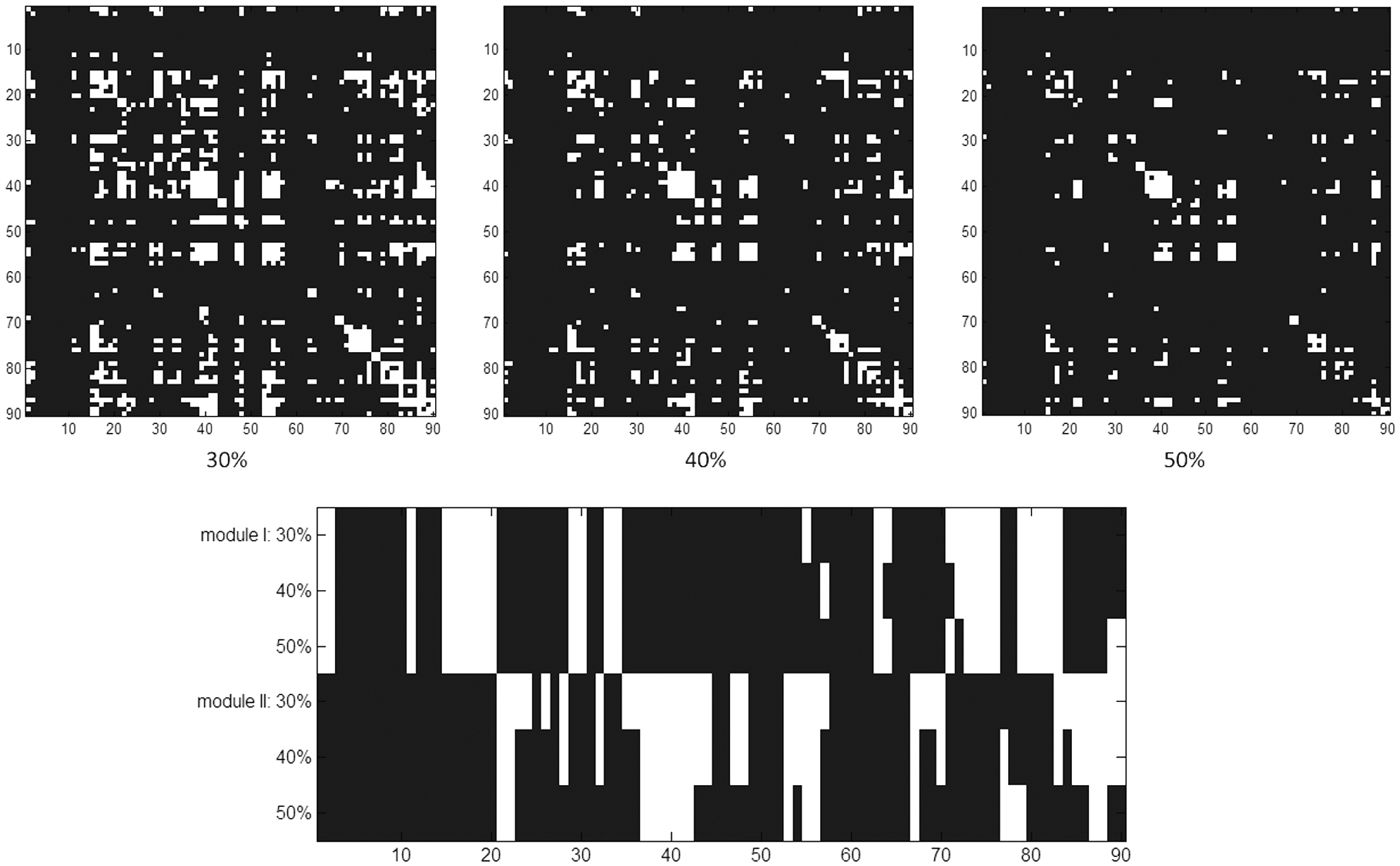
Upper row: The three binary maps were derived from the summary matrix (proportion of significant connectivity strength difference of slow-4 and slow-5, as shown in Fig. 4) by thresholding at 30%, 40%, and 50% levels (left, middle, and right, respectively). Construction was achieved by assigning a value of 1 to cells with values no less than the cutoff in the summary matrix; otherwise, 0 is assigned. The ordinate and abscissa are both ROI codes. Lower row: For the summary matrix of connectivity strength differences (Fig. 4), modularity analyses by OSLOM2 consistently revealed two community structures (upper: module 1; lower: module 2) across three different proportion thresholds. The abscissa of codes 1–90 indicated the 90 ROIs; refer to Table 1 for the code detail. White (value=1) and black (value=0) denote included and nonincluded ROIs for modules, respectively. OSLOM2, OSLOM, 2nd version.

FIG. 6.

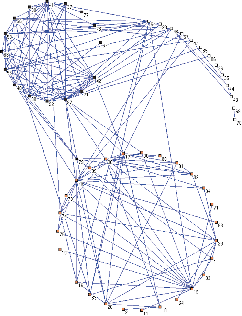
For the summary matrix of connectivity strength differences, Pajek software was used to illustrate the two community structures computed by OSLOM2 at 50% threshold. Codes 1–90 represent the 90 ROIs; refer to Table 1 for the code detail. Connections within modules are denser than those between modules. Black square: module 1; orange square: module 2; white square: nonmodular nodes. Color images available online at www.liebertpub.com/brain

FIG. 7.

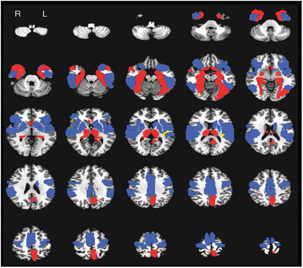
For the summary matrix of connectivity strength differences, AFNI was used to present the distribution of the two community structures revealed by OSLOM2 at 50% threshold. The community structures are superimposed on a T1 structural image in axial sections from z=−54 mm to z=66 mm, with an interslice gap of 5 mm. Blue: module 1; red: module 2. AFNI, Analysis of Functional NeuroImages software package. Color images available online at www.liebertpub.com/brain

Frequency effects on graph features of FC network

The FC of temporal courses of 90 ROIs constituted a 90×90 matrix, with each cell storing the pairwise correlation coefficient. Slow-4 and slow-5 had their own adjacency matrices. We avoided arbitrary threshold selection by assigning a series of cutoff values to sieve out the cells of lower connectivity strengths. The cutoff percentages ranged from 0% to 91% (i.e., survival percentages from 100% to 9%), and 92 binary maps were accordingly generated. For each binary map, six network indices commonly encountered in graph theory literature were calculated, including characteristic path length, global efficiency, clustering coefficient, transitivity, local efficiency, and Newman's modularity. Paired t-tests were used to examine the frequency effects of slow-4 and slow-5. Bonferroni correction was used to control for multiple comparisons, with the p-value set at 0.00054 (=0.05/92), as shown in Figure 8. Notably, the local network properties of clustering coefficient and transitivity both showed significant frequency effects across the 92 thresholds, with slow-4 smaller than slow-5. Nevertheless, slow-4 and slow-5 did not possess different effects on local efficiency. The frequency effects on the global network features of characteristic path length and global efficiency were generally negative, although with few exceptions for characteristic path lengths. The optimal modularity values did not differ in all 92 FC matrices between slow-4 and slow-5.

FIG. 8.

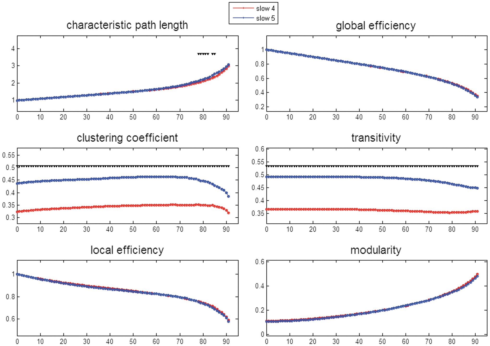
Comparison of six network features (ordinate) between slow-4 and slow-5 at thresholds of 0–91%, indicating network density from 100% down to 9% (abscissa). These graph indices were derived from the connectivity matrix of the 90 average time series from the 90 ROIs, with the value of correlation coefficient in each cell. Notably, the “thresholds” differed from those used in previous figures; 60% means that the elements of the strongest 40% connectivity strengths remained. Accordingly, each threshold was accompanied by a correspondent matrix that is further binarized to 1 (e.g., threshold 60% means 40% left) and 0 (e.g., threshold 60% means 60% removed). Black triangles pointing down symbolize the thresholded matrix that showed significant slow-4 and slow-5 differences with a corrected p-value of 0.00054 (0.05/92). Color images available online at www.liebertpub.com/brain

Betweenness centrality is a local index counting the number of shortest paths from all pairs of vertices passing through a particular node, which can be viewed as an indicator of the “hub” (Tomasi and Volkow, 2011). As other graph indices, betweenness centrality was also measured on each of the subject, for each sparsity value and for each of the two frequency bands. Figure 9 shows the absolute values of the mean differences of centrality between slow-4 and slow-5 across 92 thresholds and 90 ROIs (absolute values for better inspection; the values were not normalized by the number of off-diagonal elements 90×89 so greater than 1). The brain regions demonstrating significant slow-4 versus slow-5 differences in betweenness centrality included left cuneus (10), left IOG (15), right IOG (23), left PAL (20), left HES (11), right TPO (5), left middle temporal gyrus (MTG) (8), right MTG (28), and left TPO (medial) (TPOmed) (12). The number in the parentheses is the total number out of 92 comparisons (thresholds) surviving p<0.0001. For all brain regions showing significant centrality differences, slow-4 was less than slow-5 except for left cuneus and bilateral MTG. Figure 10 summarizes the ROI-percentage pairs showing significant centrality differences. Here the ROI-percentage means the combination of ROI code and the cutoff.

FIG. 9.

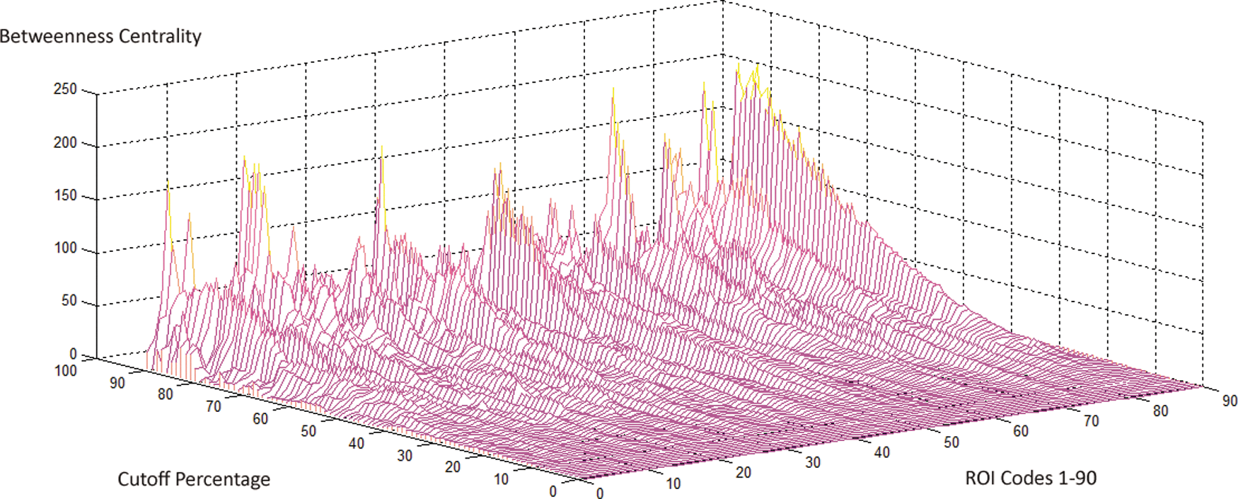
Mean differences in betweenness centrality by slow-4 minus slow-5 at 90 ROIs (1–90) and across percentage thresholds 0–91% (y-axis). The ordinate (z-axis) is the absolute value for easy appreciation. Codes 1–90 represent the 90 ROIs (x-axis); refer to Table 1 for the code detail. Color images available online at www.liebertpub.com/brain

FIG. 10.

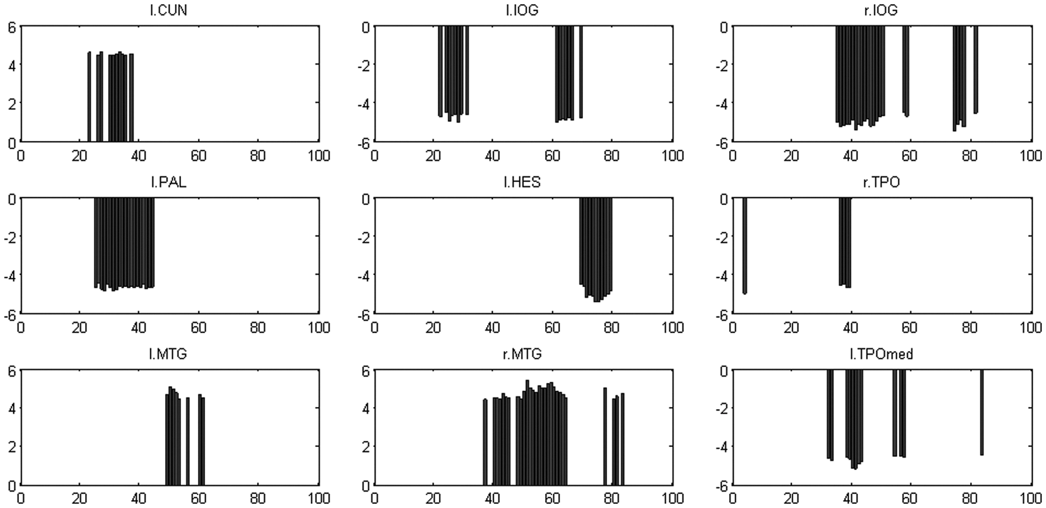
t-Statistics of slow-4 and slow-5 differences in betweenness centrality (slow-4 minus slow-5) across percentage thresholds 0–91%, and only the significant ROIs are shown. Significance was defined by p<0.0001 for at least four consecutive ROI-percentage pairs. For each significant ROI, t-values (ordinate) of the percentage cutoffs (abscissa) with p<0.0001 are illustrated. Refer to Table 1 for the abbreviation of ROI at the top of each subplot; “r” and “l” denote right and left, respectively.

Discussion

This study used fMRI to measure spontaneous brain activity in resting state and to systemically explore the neural characteristics of slow-4 and slow-5 at regional, interregional, and network levels. The aim was to examine whether these neural properties differed between slow-4 and slow-5; if differences existed, the brain structures sensitive to frequency effects were then determined. The differentiation of spectrum effects is important because EEG evidence has suggested that several rhythms can coexist in the same structures and interact with one another (Steriade, 2001). The rule, not the exception, is that a simple neural circuit in vivo can generate different kinds of rhythms that may result from local and/or distant synaptic interaction further modulated by activating systems originating in brain stem or basal forebrain. More importantly, different oscillatory patterns may represent various psychophysiological states or functions. Assuming that neural oscillations at different frequency ranges reflected themselves in BOLD at only one single spectrum seemed unreasonable. Instead, our results provided evidence that slow-4 and slow-5 BOLD signals in resting state were distinct entities. They were not divergent in every aspect but showed different properties at regional, interregional, and network levels. Similar to the conclusion of Mantini and associates (2007), we inferred that slow-4 and slow-5 may also have respective EEG signatures.

Regional effects of slow-4 and slow-5

ReHo and ALFF are both regional properties of baseline brain activity. ReHo measures the similarity of time series from voxels within a region, in contrast to FC (discussed in next section) which measures the similarity of time series between two distant regions. ReHo results at q<0.01 were generally symmetrical or situated around the midline. The ReHo results can be tentatively categorized into four categories: limbic/paralimbic system, sensorimotor-related system (pre- and post-central gyrus, paracentral lobule, supplementary motor area, inferior frontal gyrus, insula, basal ganglia, ventrolateral thalamus, and cerebellum), midline structures (anterior, middle and posterior cingulate gyrus, medial superior frontal cortex, cuneus, and precuneus), and attention-related neural correlates (superior frontal gyrus and superior parietal lobule). In the sensorimotor-related system, inferior frontal gyrus is associated with language production, action execution, and mirror neurons (Fadiga et al., 2009; Liakakis et al., 2011), whereas insula is known to play roles in interoception and homeostasis (Craig, 2003). We acknowledged that the above attribution of function was not an exhaustive account; nevertheless, the summary helped in comparing the analytical results of ReHo with other neural indices, as shown below. Interestingly, the resting dynamics in ventrolateral and mediodorsal thalamus were more strongly synchronized at slow-4 and slow-5, respectively. The functions of the two thalamic regions differ. Ventrolateral nuclei serve as the motor relay station where the pathways from the cerebellum and extrapyramidal system converge, and information is further transmitted to motor-related and parietal areas (Shinoda et al., 1993). The mediodorsal (or dorsomedial) nuclei mainly project onto the prefrontal cortex (Kuroda et al., 1998), engaging in arousal, emotion, and memory processes (Markowitsch, 1982; Watanabe and Funahashi, 2012). The EEG literature has suggested that regional spectral properties of the four central systems listed above are associated with important psychological functions. To name a few, theta oscillation can be a neural correlate of short-term memory processes in the anterior limbic system (Klimesch, 1996), EEG desynchronization at Rolandic rhythm is associated with imagination and planning of a movement (Pfurtscheller and Neuper, 1997), alpha oscillation may play active roles in saccades and selective attention (Hamm et al., 2012; Klimesch, 2012), and enhanced alpha activity can predict self-referential thoughts within the default mode network (Knyazev et al., 2012). The physiological or psychological functions of slow-4 and slow-5 of these systems are largely unknown. The correspondence of the spectrum distribution of resting fMRI and of regional EEG demands further study to clarify.

ALFF is the L1 norm of low-frequency BOLD fluctuation. We adopted the mean ALFF that standardized each voxel's ALFF with the global mean ALFF value to explore the spectrum effect. After normalization, the differences between slow-4 and slow-5 at some brain areas provided hints that their respective deviations from the global mean were dissimilar. At the more stringent criterion of FDR q<0.01, slow-4 mALFF was greater than slow-5 mALFF in caudate, thalamus, and postcentral gyrus, whereas slow-5 mALFF was greater than slow-4 mALFF in posterior cingulate gyrus. At a looser threshold, FDR q<0.05, ventromedial prefrontal, inferior frontal, and cuneus/precuneus showed smaller slow-4 mALFF. By contrast, in the inferior temporal regions, slow-4 mALFF was greater than slow-5 mALFF. The results were highly consistent with previous reports on bilateral caudate, bilateral thalamus (slow-4>slow-5), and ventromedial prefrontal cortex (slow-5>slow-4) comprising sensorimotor and midline systems (Yu et al., 2014; Zuo et al., 2010).

The abnormality of ReHo and/or mALFF has been reported in several mental conditions. Some key findings of the abnormalities are situated at where we found spectrum differences, such as limbic system in depressive disorder, trait anxiety, and bipolar disorder (Guo et al., 2011; Hahn et al., 2013; Liu et al., 2012), limbic system and caudate in schizophrenia (Hoptman et al., 2010), midline structures in panic symptom and heroin abuse (Jiang et al., 2011; Lai and Wu, 2013), limbic, midline, and sensorimotor structures in Internet addiction (Liu et al., 2010), and inferior frontal and insular regions in autism (Paakki et al., 2010). We speculated that taking a subspectrum approach as demonstrated in this study may improve delineating the brain maps associated with mental illnesses and psychological constructs.

Influence of slow-4 and slow-5 on FC

This study adopted a common approach to investigate FC. The brain was divided into 90 ROIs with the help of a parcellation scheme provided by JuBrain atlas. EPI images were preprocessed and band passed, and then the mean time series of each ROI was retrieved and used as seeds to further correlate with all voxels in the brain. Hence, 90 brain maps were constructed for both slow-4 and slow-5. After z-transformation of the correlation coefficients, paired t-tests of slow-4 and slow-5 were performed, and 90 statistical parametric maps were derived. We reduced the results of 90 statistical brain images to a summary matrix by transforming the content of the ROI pair into a proportion of significant voxels (see section FC analyses). FC strengths at slow-4 were found to be generally weaker than those at slow-5.

The raw summary matrix looked quasi-symmetrical. It was not surprising since if taking ROI A as a seed resulted in a higher proportion of significant voxels in ROI B, then conversely, taking ROI B as a seed also revealed a higher proportion of significant voxels in ROI A. It was because, first, the seed time series was the average temporal course of region that was innately representative of the composite voxels; second, spatial smoothness was applied; third, the behaviors of the voxels within an ROI were more homogenous than that between ROIs; and last, Pearson's correlation was undirectional. We symmetrized the raw summary matrix, compared the impacts of different cutoffs (30%, 40%, and 50%), and used OSLOM2 to unveil the underlying modular structures. Analyses revealed two communities that were most sensitive to spectrum effects on FC strengths; one was relevant to sensorimotor network, and the other one was concordant with the limbic system. Midline structures of the middle cingulate gyrus and precuneus were categorized into sensorimotor and limbic modules, respectively, consistent with their functions. The middle cingulate gyrus is the posterior part of anterior cingulate gyrus, and meta-analysis confirmed its role in sensorimotor functioning (Torta and Cauda, 2011). Precuneus and hippocampus have an intrinsic connection that predicts memory performance and early Alzheimer's disease (Kim et al., 2013; Wang et al., 2010).

The outputs of OLSLOM2 analyses were stable and consistent across three cutoffs (30%, 40%, and 50%). Together with the results of ReHo and mALFF, we concluded that sensorimotor, midline, and limbic systems were sensitive to spectrum effects of slow-4 and slow-5. The sensorimotor system here was used in a broader sense, containing inferior frontal gyrus, supramarginal gyrus, and insula. The brain regions associated with higher cognitive function such as dorsolateral prefrontal cortex, however, did not demonstrate different effects between the two frequency bands. We inferred that the brain systems showing slow-4 and slow-5 differences may be phylogenetically earlier in evolution to which an organism resorted to register environment (sensory), modulate inner states (limbic and midline), and respond to survival challenges (motor).

FC is known to be spectrum selective in EEG, which may also implicate disease state in depressive disorder (Fingelkurts et al., 2007; Lee et al., 2011a). Recent reports have further revealed that genetic polymorphisms also influence resting FC in a spectrum- and region-specific manner (Lee et al., 2011b, 2012). To our knowledge, only Zhang and coworkers addressed the spectral issue of FC in resting fMRI, who used machine classification of whole brain connectivity patterns to determine vascular dementia (Zhang et al., 2013). Unlike our approach, they did not delve into the details of FC maps but only constructed an adjacency matrix based on ROIs. Modular analyses based on the criteria that 30%, 40%, and 50% voxels within an ROI showing significant frequency effects disclosed consistent community structures. It is suggested that power correlation in the delta band can be the neural origin of FC in resting fMRI at primary somatosensory cortex (Lu et al., 2007). We believed that slow-4 and slow-5 FC maps may have respective electrophysiological signatures at sensorimotor, midline, and limbic systems (Mantini et al., 2007).

Influence of slow-4 and slow-5 on network features

On the basis of the mean EPI time series of 90 ROI, we constructed a 90×90 adjacency matrix by Pearson's correlation, with the value of each cell equal to the correlation coefficient of the ROI pair indicated by column and row. Graph theory is a descriptive way to summarize the features of a network, which is generally reduced to simple points called nodes or vertices, and their pairwise relationships known as edges or links. Vertices with edges bridging them are called neighbors. Based on a comparison with networks generated by a stochastic random process, graph theorists may claim the existence of structures.

Compatible with the results of FC analyses demonstrating region-specific effects, global integration indices (i.e., characteristic path length and global efficiency) generally did not show significant differences. By contrast, local segregation features (i.e., clustering coefficient and transitivity) were distinguished by slow-4 and slow-5. Considering that the connectivity strengths were stronger at slow-5 in the sensorimotor, midline, and limbic systems, sequential cutoffs made the associated structures at slow-5 more obvious than those at slow-4. These cutoffs were thus reflected in the segregation indices, consistently showing slow-5 greater than slow-4.

Local efficiency was another measure of network segregation but failed to set apart slow-4 and slow-5. This phenomenon can be because of their disparate definitions. For a target node and its directly connected vertices (indirect connections are not taken into consideration), clustering coefficient and transitivity count the triangles formed by the target and its neighbors, whereas local efficiency is based on the estimation of the shortest path lengths between two vertices where the linking path contains only the target's neighbors (Rubinov and Sporns, 2010). We regarded that local efficiency imposed a more stringent restriction on local topology, and these segregation indices summarized different aspects of local topology.

The measure of node centrality is used to evaluate the importance of local regions that interact with many other regions and may thus play a key role in facilitating integration or in resilience to injury, sometimes also named hubs. Betweenness centrality is an important indicator defined as the fraction of all shortest paths traveling through the given node in a network. The vertex that bridges disparate parts of a network usually has a high degree of betweenness centrality (Rubinov and Sporns, 2010). Out of the 90 ROIs, the values of betweenness centrality at 9 regions differed between slow-4 and slow-5 and can also be grossly grouped into limbic/paralimbic (left medial TPO, right TPO, and bilateral MTG) and sensorimotor structures (left HES, bilateral IOG, left cuneus, and left PAL). Except for MTG and left cuneus, betweenness centrality at slow-4 was smaller than that at slow-5. Our results revealed that the importance of neural nodes in a network may be changed at different spectral ranges.

Limitations and future directions

In accordance with recent studies, this project supported the distinction between slow-4 and slow-5 of resting fMRI signals. However, whether 0.027 Hz is the best breaking point for frequency division must be carefully considered. Even in the extant EEG literature, the definitions of frequency bands and sub-bands are still inconsistent and debated. Moreover, a large interindividual variability exists. This issue is difficult but unfortunately not trivial. Taking the alpha frequency band in EEG as an example, using 8–12 Hz to delineate alpha rhythm can incorporate theta rhythm for people with higher individual alpha frequency (IAF) and lose lower alpha information for people with lower IAF (Klimesch, 1999). Comparing resting and task EEG, as well as tracing the intersection of alpha and theta power spectrum, can help determine the transition between alpha and theta rhythms (Klimesch, 1999). Whether a similar objective manner can be used to determine the individual boundary of slow-4 and slow-5 is interesting to know and can affect future resting fMRI studies.

We acknowledge that our analytic strategy is not novel but just a modified strategy based on well-established analytic steam, such as temporal course extraction and FC comparisons provided by AFNI, and modularity analysis by OSLOM2. Direct comparison of the slow-4 and slow-5 90×90 FC matrices is too coarse since it ignores heterogeneity embedded in ROIs as demonstrated in this study. On the other hand, analyses based on tens of thousands of voxels are not economic and feasible, not to mention the multiple comparison correction. Nevertheless, we regard that an ideal method to tackle the spectrum issue should enable brain parcellation by voxel-wise FC (instead of predefined anatomical regions) and statistical topological comparisons that may refine our findings in future research.

Our results indicated that the spectrum effects of resting fMRI mainly aggregated in midline, limbic/paralimbic, and sensorimotor systems. The first two systems are critical in psychiatric pathogenesis, and the last two are the main targets of neurological diseases. On the basis of these findings, we suggest using a spectrum-specific approach to studying neuropsychiatry populations by resting fMRI that can help uncover underlying disease mechanisms and useful biomarkers. We also encourage elucidation of the relationship between the spectrum effects of resting BOLD dynamics and the characteristics of emotion regulation, memory consolidation, motivation, self-integration, and other mental functions closely related to limbic and midline structures.

Conclusions

This study on resting fMRI aimed to explore different effects of slow-4 (0.027–0.073 Hz) and slow-5 (0.01–0.027 Hz) on the brain. The spectrum effects were systematically examined at regional, interregional, and network levels by ReHo and mALFF, FC patterns, and network features, respectively. Our results supported previous research dividing low-frequency BOLD fluctuation into two sub-bands. For ReHo, slow-4 was greater than slow-5 in ventral brain, ventrolateral thalamus, and basal ganglia, whereas slow-5 was greater than slow-4 in inferior frontal gyrus, insula, dorsomedial thalamus, and some midline structures. For mALFF, slow-4 was greater than slow-5 in thalamus and caudate, and slow-5 was greater than slow-4 in posterior cingulate gyrus. FC analyses revealed a consistent trend that slow-4 had weaker connectivity strengths than slow-5 in brain regions reaching statistical significance by paired t-tests. Community analysis of FC results detected two modules sensitive to frequency effects: one comprised sensorimotor structure, and the other encompassed limbic/paralimbic system. Graph theoretical analysis verified that slow-4 and slow-5 differed in local segregation measures. For betweenness centrality, slow-4 was greater than slow-5 in MTG and left cuneus, whereas slow-5 was greater than slow-4 in PAL, HES, IOG, and TPOs. Although the manifestation of frequency differences seemed complicated, the associated brain regions can be categorized into limbic/paralimbic, midline, and sensorimotor systems. Future resting fMRI research addressing the three above systems either from neuropsychiatric or psychological perspectives may consider using a spectrum-specific analytical strategy. Our results provided novel insight into the spectrum specificity and complexity of the “resting” brain.

Footnotes

Acknowledgments

This work was supported by starting fund number PD13002004 supported by Hangzhou Normal University, China. We thank Dr. Green, who helped prepare this article.

Author Disclosure Statement

No competing financial interests exist.

References

Achard

, Bullmore

. 2007. Efficiency and cost of economical brain functional networks. PLoS Comput Biol, 3:e17.

Bertrand

, Tallon-Baudry

. 2000. Oscillatory gamma activity in humans: a possible role for object representation. Int J Psychophysiol, 38:211–223.

Biswal

, Yetkin

, Haughton

, Hyde

. 1995. Functional connectivity in the motor cortex of resting human brain using echo-planar MRI. Magn Reson Med, 34:537–541.

Buzsaki

, Draguhn

. 2004. Neuronal oscillations in cortical networks. Science, 304:1926–1929.

Craig

. 2003. Interoception: the sense of the physiological condition of the body. Curr Opin Neurobiol, 13:500–505.

Davidson

. 1992. Anterior cerebral asymmetry and the nature of emotion. Brain Cogn, 20:125–151.

Eickhoff

, Stephan

, Mohlberg

, Grefkes

, Fink

, Amunts

, et al. 2005. A new SPM toolbox for combining probabilistic cytoarchitectonic maps and functional imaging data. Neuroimage, 25:1325–1335.

Fadiga

, Craighero

, D'ausilio

. 2009. Broca's area in language, action, and music. Ann NY Acad Sci, 1169:448–458.

Fingelkurts

, Fingelkurts

, Rytsala

, Suominen

, Isometsa

, Kahkonen

. 2007. Impaired functional connectivity at EEG alpha and theta frequency bands in major depression. Hum Brain Mapp, 28:247–261.

10.

Guo

, Liu

, Xue

, Yu

, Ma

, Tan

, et al. 2011. Abnormal neural activities in first-episode, treatment-naive, short-illness-duration, and treatment-response patients with major depressive disorder: a resting-state fMRI study. J Affect Disord, 135:326–331.

11.

Hagemann

, Naumann

, Becker

, Maier

, Bartussek

. 1998. Frontal brain asymmetry and affective style: a conceptual replication. Psychophysiology, 35:372–388.

12.

Hahn

, Dresler

, Pyka

, Notebaert

, Fallgatter

. 2013. Local synchronization of resting-state dynamics encodes Gray's trait anxiety. PLoS One, 8:e58336.

13.

Hamm

, Sabatinelli

, Clementz

. 2012. Alpha oscillations and the control of voluntary saccadic behavior. Exp Brain Res, 221:123–128.

14.

Hoptman

, Zuo

, Butler

, Javitt

, D'angelo

, Mauro

, et al. 2010. Amplitude of low-frequency oscillations in schizophrenia: a resting state fMRI study. Schizophr Res, 117:13–20.

15.

Jiang

, Qiu

, Zhang

, Han

, Lv

, Li

, et al. 2011. Amplitude low-frequency oscillation abnormalities in the heroin users: a resting state fMRI study. Neuroimage, 57:149–154.

16.

, Saad

, Simmons

, Milbury

, Cox

. 2010. Mapping sources of correlation in resting state FMRI, with artifact detection and removal. Neuroimage, 52:571–582.

17.

Kim

, Kim

, Lee

. 2013. Hippocampus-precuneus functional connectivity as an early sign of Alzheimer's disease: a preliminary study using structural and functional magnetic resonance imaging data. Brain Res, 1495:18–29.

18.

Klimesch

. 1996. Memory processes, brain oscillations and EEG synchronization. Int J Psychophysiol, 24:61–100.

19.

Klimesch

. 1999. EEG alpha and theta oscillations reflect cognitive and memory performance: a review and analysis. Brain Res Brain Res Rev, 29:169–195.

20.

Klimesch

. 2012. Alpha-band oscillations, attention, and controlled access to stored information. Trends Cogn Sci, 16:606–617.

21.

Knyazev

, Savostyanov

, Volf

, Liou

, Bocharov

. 2012. EEG correlates of spontaneous self-referential thoughts: a cross-cultural study. Int J Psychophysiol, 86:173–181.

22.

Kuroda

, Yokofujita

, Murakami

. 1998. An ultrastructural study of the neural circuit between the prefrontal cortex and the mediodorsal nucleus of the thalamus. Prog Neurobiol, 54:417–458.

23.

Lai

, Wu

. 2013. Decreased regional homogeneity in lingual gyrus, increased regional homogeneity in cuneus and correlations with panic symptom severity of first-episode, medication-naive and late-onset panic disorder patients. Psychiatry Res, 211:127–131.

24.

Lancichinetti

, Radicchi

, Ramasco

, Fortunato

. 2011. Finding statistically significant communities in networks. PLoS One, 6:e18961.

25.

Lee

, Wu

, Yu

, Chen

. 2011a. The implication of functional connectivity strength in predicting treatment response of major depressive disorder: a resting EEG study. Psychiatry Res, 194:372–377.

26.

Lee

, Yu

, Hong

, Tsai

, Wu

, Chen

. 2011b. The effects of catechol-O-methyl-transferase polymorphism Val158Met on functional connectivity in healthy young females: a resting EEG study. Brain Res, 1377:21–31.

27.

Lee

, Yu

, Hong

, Tsai

, Wu

, Chen

. 2012. The influence of apolipoprotein E Epsilon4 polymorphism on qEEG profiles in healthy young females: a resting EEG study. Brain Topogr, 25:431–442.

28.

Leicht

, Newman

. 2008. Community structure in directed networks. Phys Rev Lett, 100:118703.

29.

Liakakis

, Nickel

, Seitz

. 2011. Diversity of the inferior frontal gyrus—a meta-analysis of neuroimaging studies. Behav Brain Res, 225:341–347.

30.

Liang

, Wang

, Yan

, Shu

, Xu

, Gong

, et al. 2012. Effects of different correlation metrics and preprocessing factors on small-world brain functional networks: a resting-state functional MRI study. PLoS One, 7:e32766.

31.

Liu

, Ma

, Li

, Wang

, Tie

, Li

, et al. 2012. Regional homogeneity within the default mode network in bipolar depression: a resting-state functional magnetic resonance imaging study. PLoS One, 7:e48181.

32.

Liu

, Gao

, Osunde

, Li

, Zhou

, Zheng

, et al. 2010. Increased regional homogeneity in internet addiction disorder: a resting state functional magnetic resonance imaging study. Chin Med J (Engl), 123:1904–1908.

33.

, Zou

, Gu

, Raichle

, Stein

, Yang

. 2012. Rat brains also have a default mode network. Proc Natl Acad Sci USA, 109:3979–3984.

34.

, Zuo

, Gu

, Waltz

, Zhan

, Scholl

, et al. 2007. Synchronized delta oscillations correlate with the resting-state functional MRI signal. Proc Natl Acad Sci USA, 104:18265–18269.

35.

Mantini

, Perrucci

, Del Gratta

, Romani

, Corbetta

. 2007. Electrophysiological signatures of resting state networks in the human brain. Proc Natl Acad Sci USA, 104:13170–13175.

36.

Markowitsch

. 1982. Thalamic mediodorsal nucleus and memory: a critical evaluation of studies in animals and man. Neurosci Biobehav Rev, 6:351–380.

37.

Paakki

, Rahko

, Long

, Moilanen

, Tervonen

, Nikkinen

, et al. 2010. Alterations in regional homogeneity of resting-state brain activity in autism spectrum disorders. Brain Res, 1321:169–179.

38.

Pfurtscheller

, Neuper

. 1997. Motor imagery activates primary sensorimotor area in humans. Neurosci Lett, 239:65–68.

39.

Reuter

, Rosas

, Fischl

. 2010. Highly accurate inverse consistent registration: a robust approach. Neuroimage, 53:1181–1196.

40.

Rubinov

, Sporns

. 2010. Complex network measures of brain connectivity: uses and interpretations. Neuroimage, 52:1059–1069.

41.

Saad

, Gotts

, Murphy

, Chen

, Jo

, Martin

, et al. 2012. Trouble at rest: how correlation patterns and group differences become distorted after global signal regression. Brain Connect, 2:25–32.

42.

Scholvinck

, Maier

, Ye

, Duyn

, Leopold

. 2010. Neural basis of global resting-state fMRI activity. Proc Natl Acad Sci USA, 107:10238–10243.

43.

Shinoda

, Kakei

, Futami

, Wannier

. 1993. Thalamocortical organization in the cerebello-thalamo-cortical system. Cereb Cortex, 3:421–429.

44.

Steriade

. 2001. Impact of network activities on neuronal properties in corticothalamic systems. J Neurophysiol, 86:1–39.

45.

Tomasi

, Volkow

. 2011. Functional connectivity hubs in the human brain. Neuroimage, 57:908–917.

46.

Torta

, Cauda

. 2011. Different functions in the cingulate cortex, a meta-analytic connectivity modeling study. Neuroimage, 56:2157–2172.

47.

Wang

, Negreira

, Laviolette

, Bakkour

, Sperling

, Dickerson

. 2010. Intrinsic interhemispheric hippocampal functional connectivity predicts individual differences in memory performance ability. Hippocampus, 20:345–351.

48.

Watanabe

, Funahashi

. 2012. Thalamic mediodorsal nucleus and working memory. Neurosci Biobehav Rev, 36:134–142.

49.

Wei

, Duan

, Zheng

, Wang

, Gao

, Zhang

, et al. 2014. Specific frequency bands of amplitude low-frequency oscillation encodes personality. Hum Brain Mapp, 35:331–339.

50.

, Chien

, Wang

, Liu

, Hwang

, et al. 2014. Frequency-specific alternations in the amplitude of low-frequency fluctuations in schizophrenia. Hum Brain Mapp, 35:627–637.

51.

, Hsieh

, Wang

, Liu

, Hwang

, et al. 2013. Frequency dependent alterations in regional homogeneity of baseline brain activity in schizophrenia. PLoS One, 8:e57516.

52.

Zang

, Jiang

, Lu

, He

, Tian

. 2004. Regional homogeneity approach to fMRI data analysis. Neuroimage, 22:394–400.

53.

Zhang

, Liu

, Chen

, Peng

, Liu

, Fan

, et al. 2013. Determination of vascular dementia brain in distinct frequency bands with whole brain functional connectivity patterns. PLoS One, 8:e54512.

54.

Zuo

, Di Martino

, Kelly

, Shehzad

, Gee

, Klein

, et al. 2010. The oscillating brain: complex and reliable. Neuroimage, 49:1432–1445.

55.

Zuo

, Xu

, Jiang

, Yang

, Cao

, He

, et al. 2013. Toward reliable characterization of functional homogeneity in the human brain: preprocessing, scan duration, imaging resolution and computational space. Neuroimage, 65:374–386.