Standing Waves as an Explanation for Generic Stationary Correlation Patterns in Noninvasive EEG of Focal Onset Seizures

Abstract

Cerebral electrical activity is highly nonstationary because the brain reacts to ever changing external stimuli and continuously monitors internal control circuits. However, a large amount of energy is spent to maintain remarkably stationary activity patterns and functional inter-relations between different brain regions. Here we examine linear EEG correlations in the peri-ictal transition of focal onset seizures, which are typically understood to be manifestations of dramatically changing inter-relations. Contrary to expectations we find stable correlation patterns with a high similarity across different patients and different frequency bands. This skeleton of spatial correlations may be interpreted as a signature of standing waves of electrical brain activity constituting a dynamical ground state. Such a state could promote the formation of spatiotemporal neuronal assemblies and may be important for the integration of information stemming from different local circuits of the functional brain network.

Introduction

“What is a seizure?” is part of a thought-provoking title of a recent contribution from Jean Gotman (2011), in which the fuzziness of definitions of epileptic seizures is emphasized and the obstacles that one encounters when trying to establish a generally valid and precise definition of these phenomena are discussed. More concretely, the author states (Gotman, 2011) that “one can conclude that some seizures are totally unambiguous, some are very uncertain, and there is continuity between the two extremes.” Due to the huge variability of clinical observations, manifold manifestations of epileptic seizures, and the currently limited possibilities of accurately and extensively mapping electrical brain activity with high spatiotemporal resolution, it remains unclear why and how seizures start, evolve, and terminate.

Penfield and Jasper (1954) proposed that paroxysmal high-amplitude electrical signals typically recorded from epileptic brains must be generated by the “hypersynchronous” activity of large groups of neurons. Since then it has in general been believed that the hallmark of epileptic seizures is a monolithic hypersynchronous dynamical state of the brain. During the last decade, however, accumulating evidence has led to this classical concept of epileptic seizures being reassessed. Several studies have demonstrated pronounced variations in synchronization between different brain areas, indicating that these aspects of epileptic seizures are dynamic phenomena (Jiruska et al., 2012; Milton, 2003).

For example, increases in correlation at seizure onset between amygdala and hippocampus (Bartolomei et al., 2002) and in mesial temporal structures (Bartolomei et al., 2004) have been detected, whereas rapid ictal discharges have been shown to be characterized by correlation loss (Bartolomei et al., 2004). A significant decrease of synchrony during the discharge period has also been reported, together with an abnormally high recoupling in posterior regions (Wendling et al., 2003). Schiff and coauthors (2005) emphasized the dynamic evolution of synchronization strength during seizures, with distinct synchronization in the initial and final phases and a successive increase of correlations toward seizure offset having been reported (Guye et al., 2006; Schindler et al., 2007a, 2008). In line with Timofeev and Steriade (2004) and Topolnik and coworkers (2003) this high synchronization level during the final part of seizures was interpreted by Schindler and coworkers (2007a) as an active mechanism for seizure termination, a hypothesis that has received additional corroboration (Schindler et al., 2007b, 2010). In contrast, however, significant correlation loss at seizure offset has been reported in extracranial data (Müller et al., 2011). The differences between these results may be due to different techniques of analysis, different electrode implantation schemes, and measurements being undertaken at different temporal or spatial scales.

In addition to these reported changes in the strength of inter-relations, the structure of inferred networks has also been shown to evolve during seizures (Ponten et al., 2007; Schindler et al., 2008). For example, the peri-ictal evolution of the functional brain network has been described as a transition from a predominantly random topology (small path length and clustering coefficient) to a more regular network (large path length and clustering coefficient) and back again (Schindler et al., 2008). Indeed, changes in the overall synchronization during seizures have been shown to be small in comparison to dramatic topological changes in derived networks (Kramer et al., 2010). The peri-ictal evolution of functional brain networks is also location dependent in the epileptic brain, with higher functional connectivity reported in regions of the seizure onset zone (Kramer et al., 2008). Two recent studies imply a decoupling of the seizure onset zone in the early phase of epileptic focal onset seizures and a reinforcement of global inter-relation at termination (Rummel et al., 2012; Schindler et al., 2012).

These contributions underline the dynamic nature of epileptic seizures. The diversity of observations reflects the large repertoire of dynamics in a complex system such as the brain where distinct phenomena may occur simultaneously on different spatial and temporal scales. However, it is also fascinating that a system composed of a tremendous number of highly crosslinked dynamical units with continuously changing parameters and external perturbations can also show constant aspects in its evolution (Buckner et al., 2008; Fox et al., 2005; Greicius, 2008; Greicius et al., 2003; Honey et al., 2009; Jann et al., 2010; Nyberg et al., 1996; Raichle and Mintun, 2006; Raichle et al., 2001; Shulman et al., 1997). Analysis of long-term interictal periods of intracranial EEG recordings, for example, indicates the existence of a stationary correlation structure, which remains stable over a period of at least 24 h (Kramer et al., 2011). Stable correlations between blood oxygenation level dependent signals, slow cortical potentials, and band limited power in interictal periods of electrocorticograms of epilepsy patients during sleep and awake states have also been reported (He, 2008). Therefore, the doubtless highly nonstationary EEG signals also contain surprisingly stable features, which are apparently related to resting state activity. The stability of the resting state activity of the default mode network, which is constantly maintained in spite of considerably large energy expenditure (Raichle, 2006; Raichle and Mintun, 2006), emphasizes its vital importance for the living organism. Hence, one may surmise that even EEG signals recorded during epileptic seizures may still contain traces of the topological structure of the default mode network.

In the present work we investigate this hypothesis by studying functional connectivity on the largest spatial scale of electrical brain activity under extreme conditions. Specifically, we study the peri-ictal transition of focal onset seizures as assessed by standard scalp recordings in order to examine the presence of temporarily stable correlation patterns amidst more dynamic aspects of the functional network.

Methods

Patient selection and data acquisition

EEG data were recorded from nine patients (four women, age range 21–45 years) suffering from pharmacoresistant temporal lobe epilepsy and under presurgical evaluation at the Department of Neurology of the Inselspital of the University of Bern. The ethics committee of the Kanton of Bern approved this retrospective study. Further, all patients gave written informed consent that their EEG data might be used for research and teaching purposes. We only included recordings with a sufficiently long pre- and postictal period and excluded EEGs contaminated by muscle artefacts. These were the only selection criteria employed in the present study (mean seizure duration=103±10 sec). Further information about the patients is displayed in Table 1.

Table 1.

Information About Patients and Seizure Duration

Patient	Age	Sex	Seizure	Duration (sec)
1	22	M	1	96
			2	122
			3	84
2	28	F	4	132
			5	204
3	45	F	6	113
			7	52
4	23	M	8	150
			9	120
			10	203
5	33	M	11	56
			12	106
6	18	M	13	40
			14	54
			15	119
7	27	F	16	91
			17	94
			18	50
8	23	M	19	73
9	21	F	20	107

Standard 10–20 montage positions (American EEG Society, 1986) were used. After passing an anti-aliasing filter with a cutoff frequency of 70 Hz and an attenuation of 24 dB/oct, the EEG signals were sampled at 200 Hz (seizure 1–12) and 256 Hz (seizure 13–20) using the earlobe reference. A/D conversion had a resolution of 16 bit. EEG seizure onset and seizure offset were visually determined by an experienced electroencephalographer (K.S.) in bipolar montage. As signals measured by electrodes Fp1, Fp2, O1, and O2 are occasionally contaminated by blink and movement artefacts, we excluded them from the present study. Hence, from the 19 standard electrodes of the 10/20 system, a total of 15 were retained for analysis.

Subsequently the data were transformed to the median reference of the retained channels in order to minimize the induction of spurious correlations that could have affected our analysis. To this end, at each time point EEG signals were ordered with increasing or decreasing size. The central value was then taken as reference value and subtracted from all signals. To diminish the influence of muscle artefacts, we applied a low-pass filter to the data with a cutoff frequency of 25 Hz. In addition, a high-pass filter with a cutoff frequency of 0.5 Hz was applied. These data sets are henceforth referred to as “broadband signals.” Ultimately, band-pass-filtered data were used, with definitions of frequency bands chosen according to Zschocke (2002) (δ=0.5–3.5 Hz, θ=3.5–7.5 Hz, α=7.5–12.5 Hz, β=12.5–25 Hz). For this purpose a fourth-order Butterworth filter was applied in forward and backward directions to minimize possible shifting of the signal phases. Further, we carefully checked the quality of the filtering process by comparing the original recording with the superposition of the filtered signals.

As a typical example we display in Figure 1 a selection of EEG signals measured with parietal, central, and frontal electrodes and transformed to zero mean and unit variance for each electrode. One clearly identifies the initial spreading of ictal activity, followed by a period of rapid discharges. Oscillations then gradually slow down toward the collective seizure offset.

FIG. 1.

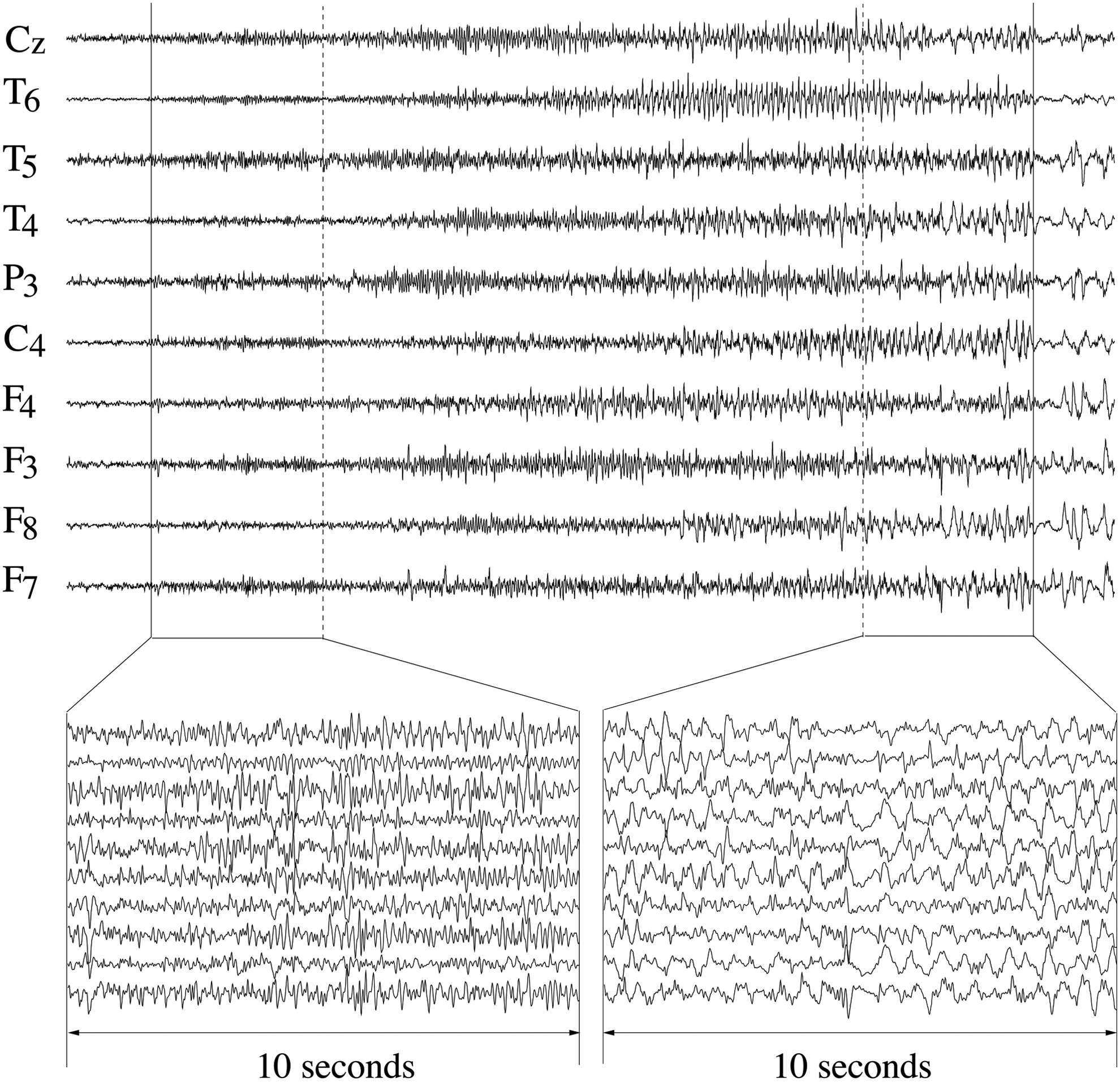
Ten representative EEG signals of seizure 7. Seizure onset and offset are marked by a vertical solid line. The additional dashed lines indicate 10-sec intervals at seizure onset and offset, which are magnified below.

Functional network and parameter settings

We define windows of T=500 and T=640 sampling points, corresponding to 2.5 sec with data recorded at 200 and 256 Hz, respectively. This data window was used to estimate the equal-time cross-correlation matrix Ĉ. The window was moved with a step width of T data points (nonoverlapping windows) over the recording.

The equal-time cross-correlation matrix can be interpreted as a weighted nondirected network or graph, where the magnitude of the matrix elements defines the functional closeness between the nodes (viz. electrode positions). In this context it is supposed that larger magnitudes of the correlation coefficient represent shorter functional paths and better information transfer between the corresponding brain regions. Although the correlation coefficient merely quantifies the similarity between finite data segments of two different data channels, by using the term “functional network” one supposes that the dynamics of the brain regions that generate these signals are also similar and, presumably, functionally connected.

We divided each recording into three intervals: a 2-min interval just before seizure onset, the seizure interval itself, and a 2-min interval starting at seizure offset. Average matrices were calculated for each of these periods and normalized using the Frobenius norm. The latter enabled us to quantify the similarity between the average matrices via the Pearson coefficient.

To exclude the possibility that the obtained results are due to volume conduction we also computed time-lag correlations. For this purpose maximum lag correlations were considered. Within a maximal time lag of 125 msec (i.e.,±25 and±32 sampling points) the maximum of the correlation coefficient between each pair of electrodes was estimated. This value of maximal time lag is consistent with García and associates (2011) and Varela and associates (2001). The average of these maximum lag correlation matrices was calculated by explicitly excluding maximum correlation coefficients with zero-lag. We additionally employed the “weighted phase lag index” (Vinck et al., 2011), a bivariate measure based on the imaginary part of the cross-spectra.

Results

Static correlation pattern and EEG reference: a case study

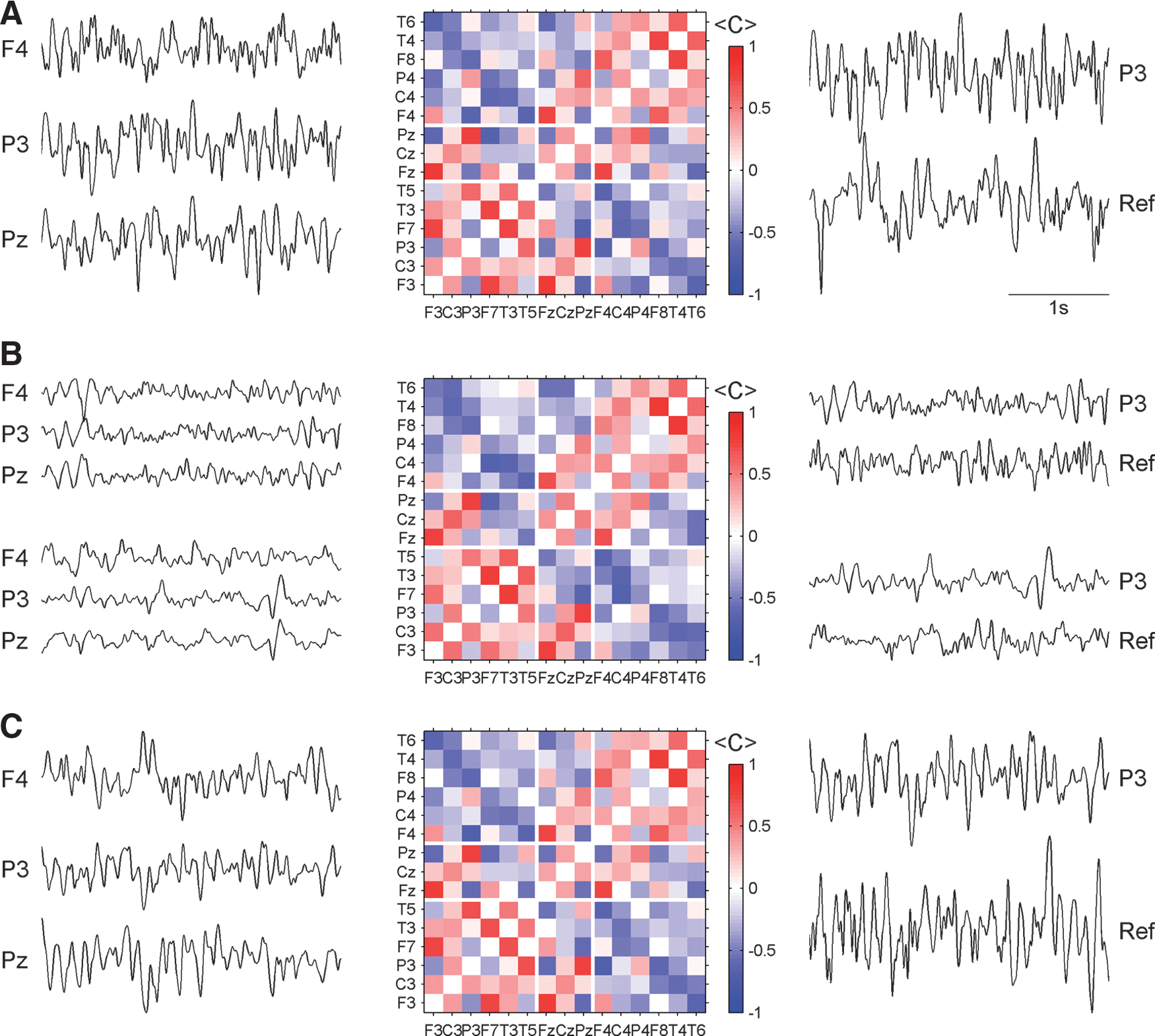
To detect stable components in the correlation structure of the peri-ictal EEGs we calculated the average of the functional network for the preseizure, seizure, and postseizure periods separately for each recording. Exemplary results for seizure 7 are displayed in Figure 2. Here and in the following figures the diagonal elements of the matrices are set to zero in order to diminish a possible distraction caused by a dominant deep red line crossing the whole matrix.

FIG. 2.

Results for the preseizure (A), seizure (B), and postseizure periods (C) of seizure 7 are presented. The left column shows examples of 3-sec segments of normalized (zero mean, unit variance) broadband signals measured by electrodes P3, F4, and Pz. From top to bottom: Segments are chosen 2 min before seizure onset, just after seizure onset, just before seizure offset, and 2 min after seizure offset. The average correlation coefficients between P3-F4 and P3-Pz are −0.63 and 0.77, respectively. The middle column shows average correlation matrices (from top to bottom) for the preseizure, seizure, and postseizure periods. Diagonal elements are set to zero in order to diminish a possible distraction caused by a deep red line crossing the whole matrices. In the right column 3-sec segments of P3 are displayed in comparison to the normalized (zero mean, unit variance) median reference. Segments are chosen at the same time periods as for the EEG signals of the left column. The Pearson coefficient between electrode signals and the median reference seems to be randomly distributed around 0 with a standard deviation of <0.1.

The most striking feature in this figure is the similarity of the correlation pattern during preseizure, seizure, and postseizure periods (Fig. 2, middle panels). Despite the fact that epileptic seizures are associated with fierce mental as well as behavioral changes and also that brain signals measured by different techniques show drastic alterations (signal power, synchronization of brain regions, blood flow, oxygen consumption, etc.) a remarkably stable mean correlation pattern of electrical activity survives during the whole peri-ictal period. Examples of (anti)correlated signals at different epochs of the peri-ictal transition illustrate the permanently pronounced inter-relationship between EEG signals after transformation to the median reference (Fig. 2, left column). It can be seen that the rhythmic quality of the signals changes notably during the peri-ictal transition from irregular oscillations during the preictal phase, rapid discharges at the initial part of the seizures, and slow waves at seizure offset and during the postseizure period. Examples of correlation values that persist despite these drastic changes in signal shape are the marked correlation between signal P3 and Pz and the pronounced anticorrelation between P3 and F4. This remains true for other electrode pairs with pronounced average correlation coefficients as indicated by the average matrices, or when different time intervals are chosen.

It is well known that different EEG references may induce characteristic spurious synchronization (Guevara et al., 2005; Schiff et al., 2005) and also that correlation patterns may be drastically influenced by certain reference schemes (Rummel et al., 2007). In light of this we sought to closely examine the inter-relation between the reference and EEG signals. The right panels of Figure 2 show exemplary segments of the median reference in comparison to the signal P3 after transformation to the median reference. Segments were chosen at the same time epochs as for the comparison of electrodes F4, P3, and Pz. No strong inter-relation between the reference signals and P3 can be recognized.

We tested for significant correlations between the median reference and all EEG electrodes. For this purpose we generated surrogate data, which represent the null hypothesis of zero genuine correlations. Such surrogates share the same linear univariate properties as the original data, but all linear inter-relationships between the signals are destroyed. This can be achieved by randomizing the Fourier phases of the signals but maintaining power spectra and amplitude distributions (Schreiber and Schmitz, 2000). Comparing the set of correlation coefficients derived from the surrogate data and the set computed from the original data we found no significant difference in the distributions. Consequently we conclude that no genuine correlations are induced by the EEG reference chosen in this study.

This is to be expected since the median value of all EEG signals is presumably almost always close to zero; therefore, on the (time) average the reference signal causes only tiny modulations to the original signals. Further, as the median value is almost always given by a different EEG channel, the induction of global correlations over a time window of 2.5 sec is not likely. Both arguments suggest that the median reference is less prone to inducing spurious correlations between a large number of electrodes, although a more formal proof of this statement is still lacking. However, as an additional verification we calculated the average correlation pattern for other EEG references including the global average, the mean between electrodes F3 and F4, and the Hjorth montage. As expected, for the global average we find quantitatively almost the same results as those shown in Figure 2. When the mean of F3 and F4 is used, only slight changes in correlation are detected for those coefficients where one of the reference electrodes is involved. The Hjorth montage on the other hand causes some distortions to the correlation pattern shown in Figure 2. The surface Laplacian theoretically reduces spurious correlations between proximal electrodes (Srinivasan et al., 2007). However, the Hjorth array in a sparse configuration such as the 10/20 system provides only a crude approximation to the Laplacian and can introduce spurious inter-relations when reference electrodes overlap (Rummel et al., 2007). In summary, we could not find a significant influence of the EEG reference.

Spatial correlations and standing waves

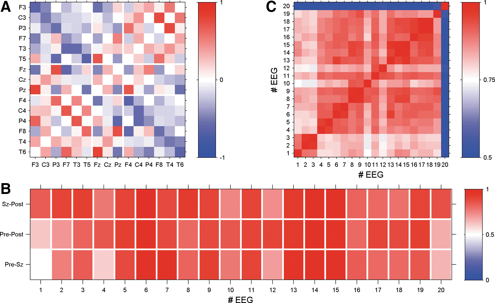
In light of the similarity of the averaged correlation matrices of Figure 2, we sought to compare the correlation pattern between each of the three epochs. To this end a grand average correlation matrix was formed for each of the three epochs and each of the twenty EEGs. To quantitatively compare the resulting matrices we estimated the Pearson correlation between the correlation matrices for each EEG. The results for all 20 EEGs are summarized in Figure 3A. In all cases, the Pearson coefficients between each pair of matrices are considerably high. Even the minimal value detected for the comparison of the average matrix derived from the pre- and postseizure periods of EEG 4 is notably high (C=0.62). Since the correlation matrices over the three epochs are so similar, we sought to also examine the average correlations over the entire peri-ictal period. An example of the outcome of such an average of the peri-ictal EEG of seizure 7 is illustrated in Figure 3B.

FIG. 3.

(A) Pearson coefficients of the three possible pairs of correlation matrices averaged over the preseizure, seizure, and postseizure intervals. (B) Peri-ictal average of the correlation matrix derived from seizure 7. Diagonal elements are set to zero.

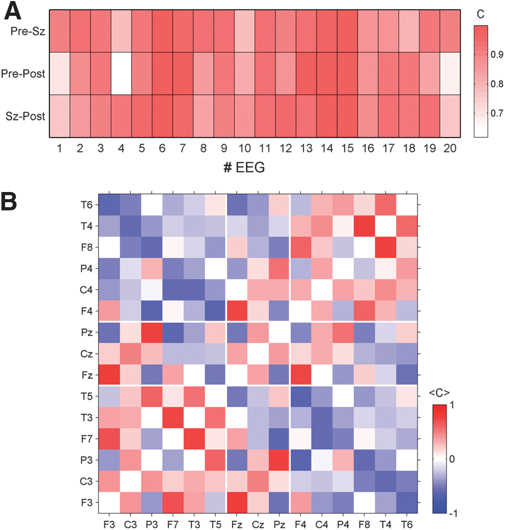
Inspecting this result in more detail it becomes obvious that the whole pattern shows an intriguing mirror symmetry between the left and right side (compare, e.g., the bottom left and top right quadrants of Figure 3B. Note that in the 10/20 system odd-numbered channels are situated on the left, and even-numbered channels on the right.). In the present case, the seizure onset zone is in the right hemisphere, but we could not find a significant asymmetry, indicating the hemisphere containing the epileptogenic zone in this, or in other cases. Hence, it seems that the seizure onset zone does not significantly alter the average correlation pattern measured by extracranial electrodes.

Signals recorded from the same hemisphere are typically positively correlated. Only a few intrahemispheric correlations have negative sign, namely, between some posterior and anterior electrodes. In this example, P3 is anticorrelated to F3 and F7 and while T5 is anticorrelated to F3. The same pattern of anticorrelated signals is also found in channels of the right hemisphere (Fig. 3B, top right quadrant). On the other hand, direct interhemispheric connections are predominantly negative. Only a few direct interhemispheric inter-relations (e.g., homologue electrode pairs) have positive sign (namely, F3-F4 and P3-P4). It can be seen that correlations between lateral and central electrodes may have either positive or negative signs. Areas close to the central electrode positions (F3, C3, P3 and F4, C4, P4, respectively) are correlated to Fz, Cz, and Pz, while more lateral electrode sites (F7, T3, T5 and F8, T4, T6, respectively) are by trend anticorrelated to the central contacts.

Roughly speaking, one might associate these observations with a standing wave on a two-dimensional elastic tissue, where on the average oscillations within each side (hemisphere) are in phase with each other, while the two opposing sides vibrate permanently in antiphase. The contra-oscillation is more pronounced between the most lateral regions of the brain. This simple picture of a standing wave of electrical activity is further supported by the EEG segments shown in Figure 2. Although the oscillations are quite irregular (in contrast to the nearly harmonic vibrations of an elastic membrane) one recognizes that signals recorded by F4 and P3 are oscillating mainly in antiphase, while signals P3 and Pz most often oscillate in phase. Of course, this association is merely a cartoon of the more complex pattern extracted from the EEG signals, but it could help to visualize some prominent features of the stationary oscillating dynamics of electrical brain activity.

Case specific or generic?

So far we have demonstrated that in each case a stationary correlation structure exists and we have presented detailed results for EEG 7. It remains to be shown whether this pattern reflects a patient-specific characteristic of electrical brain activity or whether it represents more general features of a generic pattern across patients. To quantify possible similarities between the peri-ictal averages we calculated the Pearson coefficients for all possible pairs of peri-ictal averaged correlation matrices of the 20 EEG recordings. Results of this analysis are shown in Figure 4.

FIG. 4.

(A) Pearson coefficients of all pairs of peri-ictally averaged correlation matrices of all 20 recordings. (B) Peri-ictal average of the correlation matrix derived from seizure 20. Diagonal elements are set to zero.

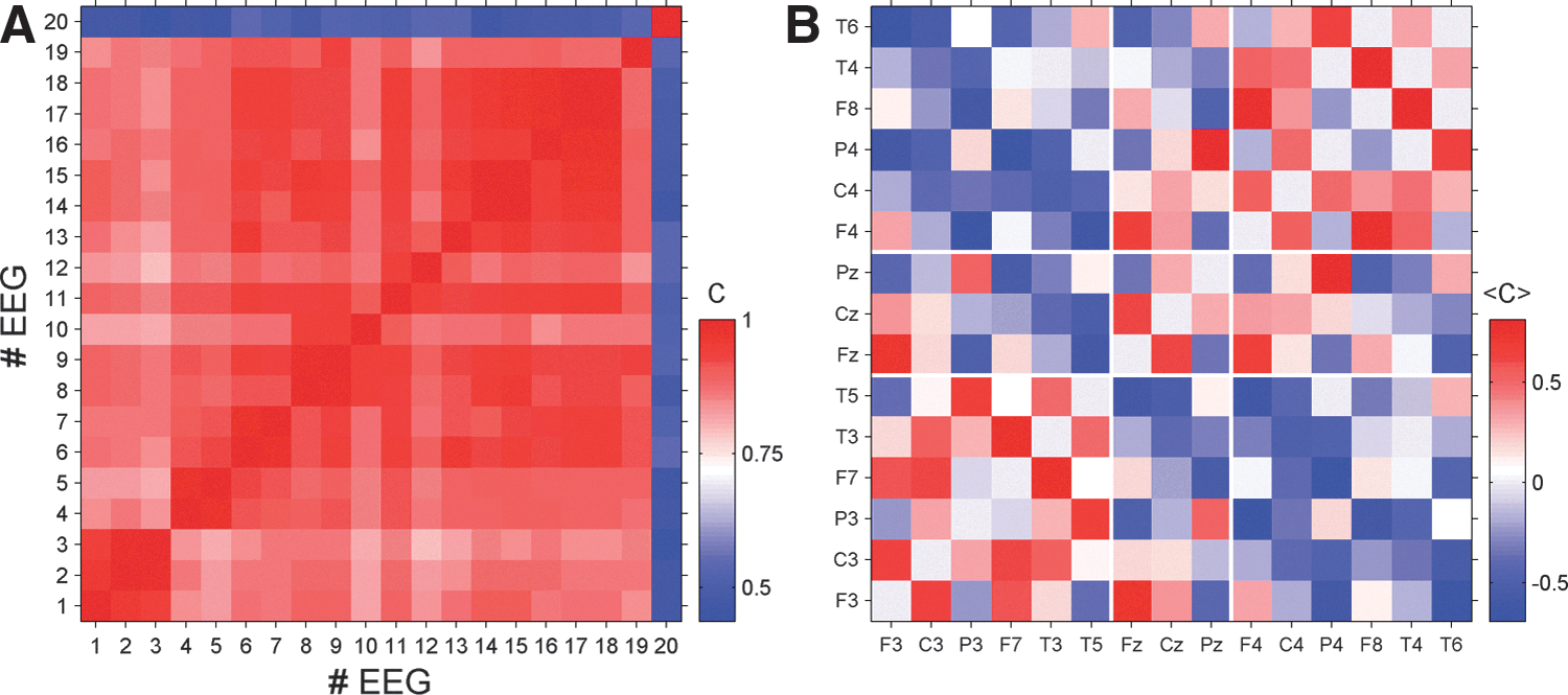
As expected, average correlation matrices derived from EEGs of the same patient possess the largest Pearson coefficients, which indicates the highest level of similarity. However, surprisingly high values are also found for correlation matrices derived from EEGs of different patients. Pearson coefficients are in most cases above 0.8. Only EEG 20 seems to be an exception and apparently the average correlation structure of this case represents an outlier. Nonetheless, the average Pearson coefficient between the correlation structure of EEG 20 and that of the other recordings is about 0.58 and therefore it is not as low as the visual impression of Figure 4 would suggest. These values are calculated by disregarding the diagonal values that otherwise would inflate the similarity.

To examine this more carefully we show in Figure 4B the peri-ictal average of the correlation matrix of EEG 20. Although it is the “worst case” in the present data, we find an intriguing similarity to the pattern found for seizure 7 (compare Fig. 3B) and, according to Figure 4A, the average correlation structures of the remaining 19 EEGs. Intrahemispheric correlations are mainly positive while direct inter-relations between the hemispheres are predominantly negative. Signals recorded from electrodes close to F3, C3, and P3 (and respectively F4, C4, and P4) tend to be positively correlated to central contacts, while the most lateral electrodes are basically anticorrelated to Fz, Cz, and Pz. Even details of the pattern found for seizure 7 are replicated in the correlation pattern of seizure 20. Pronounced correlations in the case of seizure 7 also show high values with the same sign in case 20. Qualitatively, both matrices (and also the others) are the same. The main difference consists in the correlation strength (note the different color scale in Fig. 4B compared with Fig. 3B). The pattern found for seizure 20 is somewhat less pronounced. However, in conclusion we can state that the average correlation structure found for seizure 7 is universal in the sense that we found similar patterns for all 20 recordings considered in the present study.

Do different brain rhythms generate different mean correlation structures?

Slow rhythms such as those of the δ-band are associated with large wavelengths, covering a larger spatial range, and they are therefore able to produce long-range correlations. On the contrary, the influence of fast oscillations, associated with shorter wavelengths, is restricted to shorter spatial scales. It is therefore assumed that there is a strong relationship between the spatial coverage of synchronized activity and the synchronizing frequencies (von Stein and Sarnthein, 2000), such that faster frequency bands have shorter interaction ranges and more localized synchronization phenomena.

The stationary correlation structure found for broadband signals contains short- as well as long-range correlations. Are different parts of the observed average correlation structure generated by different brain rhythms? If so, the average correlation pattern extracted for different frequency bands should be qualitatively different. To answer this question we repeated the analysis for each of the classical frequency bands separately. An exemplary picture for band-pass-filtered data of EEG 7 is provided in Figure 5. The findings are again generic in the sense that for the other EEGs of our data pool we find similar results.

FIG. 5.

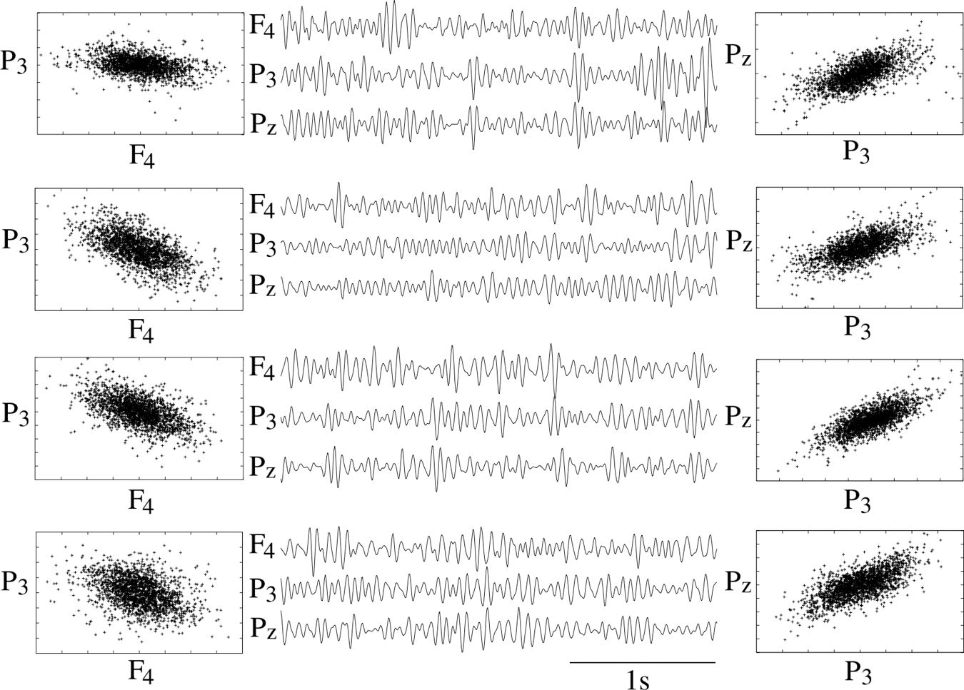
Left and right columns: Examples of 10-sec normalized (zero mean, unit variance) β-band EEG segments of electrodes P3, F4 (left column) and Pz, P3 (right column) of seizure 7 as scatter plots. In the central column the time course of the first 3 sec of the 10-sec windows of electrodes F4, P3, and Pz is shown. From top to bottom: 2 min before seizure onset, just at seizure onset, just before seizure offset, and 2 min after seizure offset.

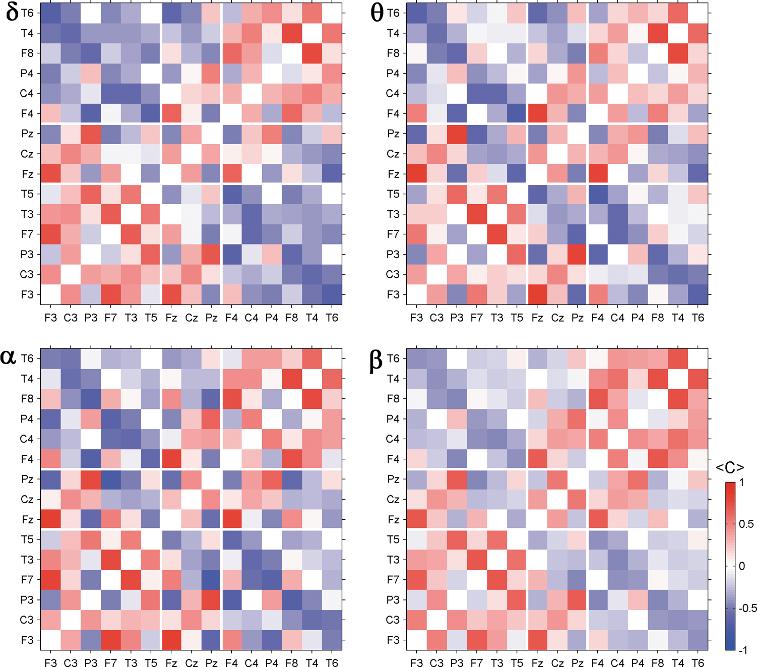
The similarity of the matrices derived from different frequency bands is remarkable. In all cases the same long- as well as short-range correlations emerge, although to a slightly different degree. Again, intrahemispheric signals are mainly correlated while direct interhemispheric signals are mostly anticorrelated. In our cartoon of an irregularly vibrating elastic tissue, we expect to see a similar standing wave for different frequency bands on the average. Figure 6 provides a further illustration of this situation and shows segments of β-band signals measured by electrodes F4, P3, and Pz and corresponding scatter plots. The segments stem from the same epochs as the EEG fragments shown in Figure 2. The peri-ictal average of the Pearson coefficient of F4 and P3 is −0.44 and that of P3 and Pz is 0.68. By visual inspection one can observe the positive and negative inter-relations between the signals, and hence, one may visualize the strict in-phase and antiphase oscillations of the electrical potential measured at these electrode positions.

FIG. 6.

Peri-ictal average of the correlation matrix for different frequency bands. The Greek letter indicates the corresponding frequency band. Diagonal elements are set to zero.

Discussion and Conclusions

The main finding of the present study is the detection and characterization of a stationary skeleton of spatial inter-relations between EEG signals, which remains stable even during the extreme dynamical changes associated with epileptic seizures. In short, correlations between signals measured from the same hemisphere are mostly positive. In contrast, interhemispheric correlations are predominantly negative with the exception of some homologue electrode pairs.

Volume conduction and choice of reference

Stable inter-relations in scalp EEG were also found in a recent study (Chu-Shore et al., 2012), in which multiday recordings of five healthy subjects were analyzed. In the study of Chu-Shore and colleagues (2012) maximum correlations within time lags of up to 200 msec were estimated and the functional connectivity network was analyzed by studying properties of the adjacency matrix such that the sign and strength of correlations were disregarded. Inhomogeneities in the average binary network were interpreted as temporarily stable couplings between different sites of the brain. The authors reported that average binary networks of the same person measured in different physiological states (awake, deep sleep, REM sleep, etc.) are strongly correlated whereas a high variability of template network structures between subjects was found.

On the contrary, our result based on zero-lag correlations indicates the existence of a generic inter-relation structure. This structure remains stable not only during very different physiological states within an individual (i.e., ictal and nonictal activity [Fig. 3]) but is also found to have a surprisingly high similarity between subjects (Fig. 4). We note that in the present study the weighted functional network as well as phases are accounted for, the latter in terms of the sign of correlations. We should therefore ask whether qualitative differences between our results and those reported in Chu-Shore and coauthors (2012) are due to differences in the analysis method, or whether they could arise spuriously, for example, due to volume conduction effects.

Chu-Shore and coauthors (2012) explicitly discarded zero-lag correlations in order to diminish the influence of the chosen EEG reference (global average in that case) and volume conduction. A worst-case scenario for the influence of the median reference on our results can be envisaged in hypothetical scenario that electrical activity in the brain is distilled into a single strong dipole in one hemisphere. In that case, and in the absence of contributions from independent activity in the contralateral hemisphere, (anti)correlations between hemispheres will be strong since essentially the same signal (or its antiphase) is compared. Crucially, however, in that case one would also expect significant correlations between each signal and the median reference. This is because the median reference would also be contributed to most strongly by the high amplitude, dominant activity of one hemisphere. Since we find the correlations between EEG signals and the median reference to be equivalent to surrogate data, we conclude that the choice of the median reference does not significantly distort our observations of a stable correlation structure.

To investigate contributions from instantaneous effects like volume conduction we also calculated maximum lag correlations. Assuming that the quasi-stationary approximation of the Maxwell equations provides a good description for the electrical activity reflected in EEG signals (Plonsey, 1967) volume-conducted electrical activity measured from two spatially separated sensors has zero (or negligible) delay (Stinstra, 1998). Therefore, a conservative strategy to avoid volume conduction effects is to exclude zero-lag inter-relationships (Nolte et al., 2004). Since we are studying cross-correlation rather than time series measures based on phase, we did not further analyze the time lags at which maximum correlation occurred. Instead we focused on the correlation coefficients and averaged each of the matrix elements separately over the resulting peri-ictal transition. In this calculation we did not impose a minimum time lag, but excluded all maximum zero-lag correlations from the averaging process. This led to ∼15% of the matrix elements being disregarded. We note that imposing a small minimal lag would not assure that instantaneous interactions are excluded from the analysis, at least not for broadband data as in the present case, where slow frequencies may play a dominant role and the minimal lag may be much smaller than half of the cycle period. On the other hand, allowing zero time lags during the maximization procedure but excluding them from the average provides an effective filter for the exclusion of all instantaneous interactions. The corresponding results are summarized in Figure 7.

FIG. 7.

Presentation of the results of maximum lag correlations for broadband signals. (A) Peri-ictal average of the maximum lag correlation matrix of seizure 7. (B) Pearson coefficients of the three possible pairs of maximum lag correlation matrices averaged over the preseizure, seizure, and postseizure intervals. (C) Pearson coefficients of all pairs of peri-ictally averaged maximum lag correlation matrices of all 20 recordings.

Figure 7A shows the exemplary average maximum lag correlation matrix of seizure 7. The similarity of the correlation structure to the one shown in Figure 3B is apparent. As in Figure 3A we compared the averages taken over the preictal, ictal, and postictal periods (Fig. 7B). For all 20 recordings we find a high similarity between the three periods for all recordings. Finally, the quantitative comparisons between the 20 peri-ictal averages (Fig. 7C) confirm the results already obtained for zero-lag correlations. Repeating the analysis for each of the classical EEG bands separately we observe pronounced correlation patterns with a comparable spatial distribution as shown in Figure 7A, although for high-frequency bands the pattern appears occasionally almost exactly reversed, such that interhemispheric maximum correlations are dominantly positive and intrahemispheric maximum correlations are mainly negative. We attribute this to time lags of τ/2, 3τ/2,…, where τ is the average period of the band-pass-filtered data. Shifts of approximately half of the cycle length simply reverse the sign of the correlation pattern. However, the distribution of correlation and anticorrelation within the average matrix shows the same spatial structure as found for zero time lags.

As additional test we estimated the weighted phase lag index (WPLI) (Vinck et al., 2011), which is an improved version of the imaginary part of the coherency (Nolte et al., 2004). Volume conduction activity may influence the spectral relationships of signals detected from spatially separated sensors and consequently it potentially alters the cross-spectra of two signals (Nolte et al., 2004; Stam et al., 2007). However, possible changes affect solely the real part of cross spectra. Volume conduction may cause a positive or negative shift on the real axis of the cross spectrum of two signals, which corresponds to a phase difference of 0° and 180°, respectively (Stam et al., 2007; Vinck et al., 2011). Therefore, measures exclusively based on phase differences (Hocke et al., 1989; Lachaux et al., 1999; Mormann et al., 2000; Rosenblum et al., 1996) are vulnerable to the influence of volume conduction, as the instantaneous phase of a signal is determined by its Fourier phases (Hramov et al., 2005), which are given by the ratio of the imaginary and real part of the corresponding Fourier coefficients.

Therefore, the original proposal of Nolte et al. (2004) was to consider the imaginary part of the cross spectra, which is zero for phase differences of 0° and 180°. Stam (2007) proposed the phase lag index as a measure with an improved sensitivity for the detection of genuine phase relations. Finally, the WPLI was proposed, which turns out to (1) be more robust against noise, (2) show a higher sensitivity for the detection of genuine phase relationships, and (3) is a normalized measure, which takes values between zero and one. Therefore, random contributions caused by finite data segments or fluctuating genuine inter-relations are not averaged out while estimating a mean inter-relation matrix over the whole peri-ictal interval. Instead, it is expected that the average WPLI matrix shows a considerable bias. Nevertheless, by drawing the average WPLI matrix and the absolute values of maximum lag correlations we observe similar structures (results not shown).

Consequently, considering that volume conduction is effective instantaneously (within the time resolution of the measurement) this phenomenon cannot be the sole explanation for the stationary correlation pattern presented in the previous sections.

Despite our use of lagged correlations as an additional measure, there are multiple reasons that motivated our use of zero-lag correlations for the body of this work.

First, volume conduction is not the only mechanism that may yield zero-lag correlations. For example, in Fischer and colleagues (2006) it was shown that long-range zero-lag correlation between oscillators could be generated by a third dynamical element acting as a relay. Although the main theoretical and experimental part of this study refers to coupled laser systems, model calculations for three different types of Hodgkin–Huxley neurons were also provided. An example of such a mechanism is presented in Gollo et al. (2011) where zero-lag corticocortical theta synchronization was investigated and the potential role of the hippocampus as a “dynamical trigger” was demonstrated. Since the pioneering work of Gray et al. (1989) where long-range zero-lag synchronization was observed in cat visual cortex (see also Roelfsema et al., 1997) a large amount of evidence has been reported that zero-lag synchronization is crucial for coordinating information processing between cortical areas. For a recent review about this subject see Gollo and associates (2013). Therefore, zero-lag inter-relations are not necessarily exclusively due to volume conduction and simply discarding them might neglect an important aspect of neuronal information processing.

Second, neurons communicate via synaptic connections. Under integrated input of its inhibitory and exhibitory synapses a neuron generates action potentials, the hallmark of longer-distance signal transfer in neuronal networks. However, neurons are also exposed to electric fields, which may influence information flow via axons and dendrites. Thus, the question arises as to whether such electric fields, which may strongly and rapidly fluctuate in space and time, may have an influence on the behavior of neuronal assemblies. Do electric fields indeed interfere with information transfer and are thus an undesired sideproduct of neuronal activity? Or—on the contrary—do local field potentials even play a constructive role in information transfer, that is, may neurons take advantage of their presence?

Recently several studies have reported that endogenous electric fields provide an effective (and maybe indispensable) mechanism for a rapid orchestration of neocortical spatiotemporal synchronization patterns (e.g., Anastassiou et al., 2010, 2011; Fröhlich and MecCormick, 2010; Marshall et al., 2006; Ozen et al., 2010; Radman and Nicholson, 2007; Weiss and Paulsen, 2010). Although the magnitude of local fields is considerably lower than the typical threshold potential of a neuron (Anastassiou et al., 2010; Fröhlich and MecCormick, 2010) they still may modulate spike timing of single neurons via ephaptic coupling (Radman and Nicholson, 2007) as well as the collective neuronal dynamics of entire neuronal populations (Fröhlich and MecCormick, 2010; Weiss and Paulsen, 2010). Endogenous local fields modulate neuronal membrane potentials on a subthreshold level (Fröhlich and MecCormick, 2010; Ozen et al., 2010; Weiss and Paulsen, 2010) and thereby influence network activity. In this way, a feedback loop may be established (Fröhlich and MecCormick, 2010), which may promote global synchronization of large neuronal assemblies. Such endogenous fields mediate a kind of cortical “self-monitoring” (Weiss and Paulsen, 2010), which seems to be particularly relevant for low frequencies below 8 Hz (Anastassiou et al., 2011). Hence, it is conceivable that endogenous fields play an active and constructive role during information processing, as, for example, memory tasks during waking state (Kirov et al., 2009) or sleep-assisted memory consolidation (Marshall et al., 2006).

Standing waves and temporal modulations

In summary we observe that the basal operational mode of the brain activity is not a decorrelated dynamical state but is characterized by a well-defined spatial inter-relationship, whereby strong short- as well as long-range (anti-)correlations are established. According to our findings it seems that in the language of dynamical systems the “attractor” of electrical brain activity can be represented by a limit cycle. The observed pattern resembles the characteristics of a standing wave, whereby the oscillation of the electrical scalp potential between the two hemispheres acts in phase opposition. Consequently, the temporal evolution of brain activity manifests itself via transient deformations of this dynamical “ground state.” Such behavior is reminiscent of the vibration of an elastic membrane, in which a basal mode of stationary oscillations is continuously deformed by fluctuations on all spatial scales ranging from small ripples causing local perturbations, to large waves warping the entire tissue. Nunez (2000) conjured the picture of the surface of a rough ocean in order to illustrate the superposition of the different Fourier modes (viz. harmonic oscillations) into which the EEG signals can be decomposed.

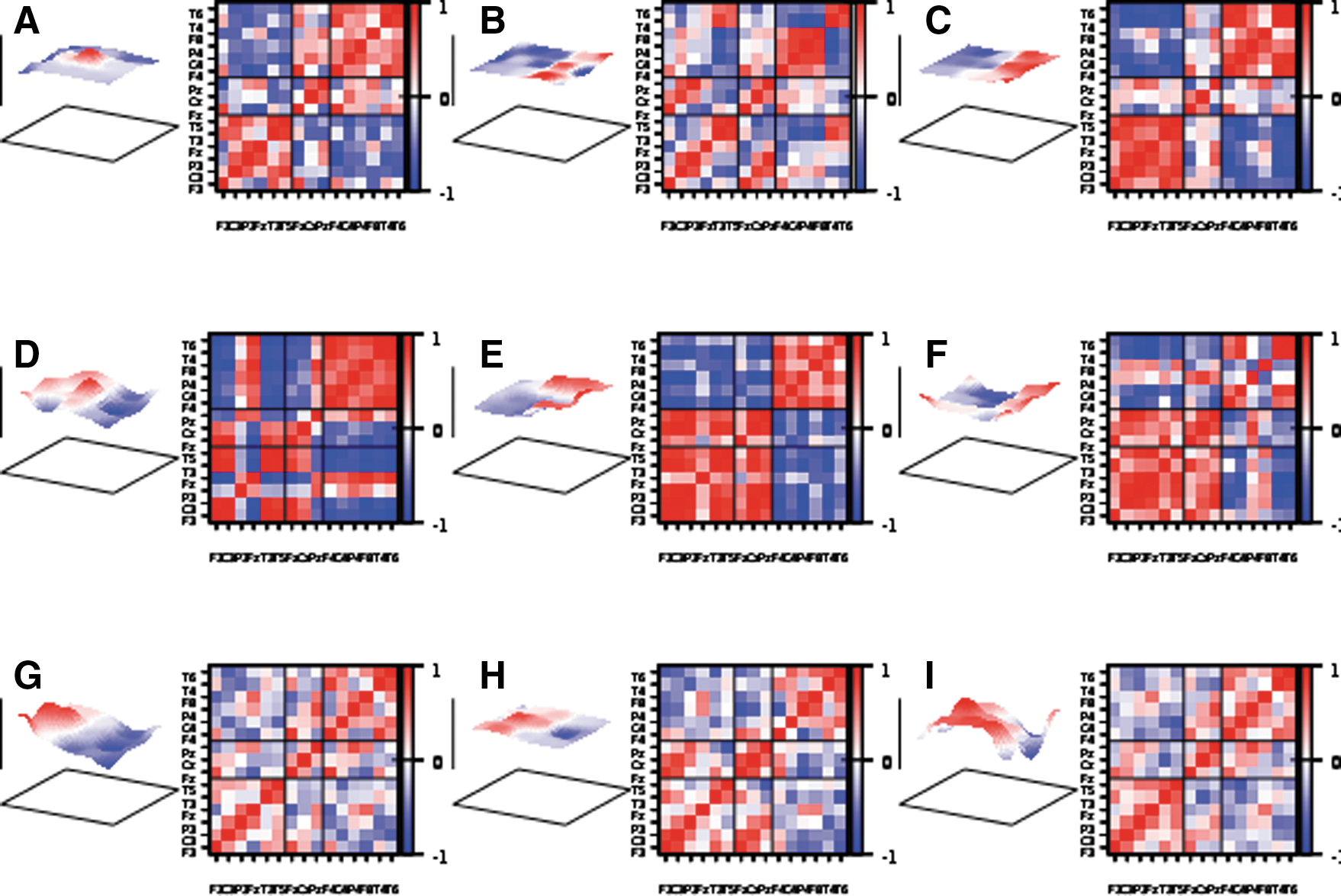
We present a visualization of this situation for the example of recording 7 in Figure 8. Additionally, Supplementary Video S1 (Supplementary Data are available online at www.liebertpub.com/brain) of the normalized electrical brain activity for frequencies below 2 Hz and the corresponding correlation patterns is provided.

FIG. 8.

The zero-lag correlation matrix estimated over a time window of 201 data points (∼1 sec) of seizure 7 for the broadband signal (A–C), frequencies below 2 Hz (D–F), and the β-band (G–I). An instant of time ∼30 sec before seizure onset (A, D, G), during the central part of the seizure (B, E, H), and ∼30 sec after seizure termination (C, F, I) were chosen. Diagonal elements are set to zero. The normalized EEG recordings from the 15 electrodes considered in this study are represented as an elastic membrane. From the normalized electrical potential at each electrode side isolines are estimated (using the splot command of gnuplot with the pm3d option). On a 100×100 grid the following coordinates define electrode positions: F3-(30,80), C3-(30,50), P3-(30,20), F7-(10,90), T3-(10,50), T5-(10,10), Fz-(50,75), Cz-(50,50), Pz-(50,25), F4-(70,80), C4-(70,50), P4-(70,20), F8-(90,90), T4-(90,50), and T6-(90,10). The membrane figures represent a snapshot at data point 101 of the actual data window. The orientation of the head forms an angle of 45° toward the screen plane.

Figure 8 shows a snap shot of the EEG signals represented as an elastic membrane and the zero-lag correlation matrix for different filtering configurations. Although the frequency content of the signals shown in the three rows of Figure 8 is quite different, the basal mode of a counter oscillation between the hemispheres is clearly visible in all cases. The corresponding correlation matrices document the pronounced intrahemisphere correlation and interhemispheric anticorrelations particularly for frequencies below 2 Hz.

Local information processing versus global dynamics

Considering that the central nervous system permanently regulates vitally important processes, it could be more energy efficient for the brain to maintain an oscillating mode on the average, such as a standing wave, rather than continuously avoiding the convergence to a fix point of zero activity. In fact, such a limit cycle attractor might not only be more economical in terms of energy consumption, but could also assure more efficient functionality of the brain.

Neural network dynamics operate by excitatory and inhibitory synaptic action. In this way, and by Hebbian learning, local networks that assume the elaboration of specific tasks emerge. Since the Hebbian mechanism aids the optimization of the topological structure of interconnections it is a reasonable assumption that local networks are also formed dynamically. Such networks may be localized; they may overlap or may occupy distinct, apparently disconnected regions of the cortex. In this scenario the standing wave acts like a dynamical ground state promoting the formation of spatiotemporal neuronal ensembles, which are “bounded by synchrony” (Singer, 1993, 2001). Such local networks may operate on different time scales; that is, they may have quite different dominant Fourier components (Nunez, 2000).

In this way the segregation of the whole neuronal network in task-specific local subunits is promoted, where locality refers to space as well as time. On the other hand, information processing requires the coordinated interplay of dynamical segregation and global integration of local network activity (Nunez, 1995; Tononi, 2004; Tononi and Edelman, 1998). Such integration processes require a precise timing and short reaction times, in order to combine the complex spatiotemporal activity of numerous local structures to an optimized global response.

If cell ensembles oscillate with different mean frequencies, namely, if they apparently present temporarily segregated local networks, then this does not necessarily imply independent dynamics. “Binding by resonance” constitutes a general mechanism by which cell assemblies selectively interact in multiple different matching frequencies. In Hoppensteadt and Izhikevich (1998) and Izhikevich (1999) numerical evidence has been provided that weakly coupled oscillators may strongly interact when their characteristic frequencies obey specific resonance relations. This framework is sufficiently general that it might be realized by the communication between local neural networks operating in different frequency ranges (Nunez and Srinivasan, 2006a, 2006b). For instance, it is conceivable that via such a coupling scheme the instantaneous phase of a slow-frequency band (e.g., theta activity) modulates the power of fast oscillations as high gamma activity (Canolty et al., 2006). Hence, such a general scheme not only illustrates a possible mechanism for the dynamical formation of operational subunits, but additionally provides an explanation of how assemblies operating on different mean frequencies may communicate.

Information processing requires ever-changing synchronous activity of neuronal populations. Coming back to the earlier-mentioned constructive role of endogenous fields the question arises whether they participate actively in such processes and what constitutes the fast and efficient mechanism that permits the recruitment or dismissal of neuronal assemblies. One possible explanation might be binding by resonance, where slow modulations of local fields may trigger the spiking of individual neurons (Radman and Nicholson, 2007) or entire populations (Ozen, 2010). On the other hand, individual neurons have preferred possibly narrow frequency ranges where they show optimal response to external stimuli (Hutcheon et al., 2000). Endogenous fields could use such resonance-like behavior by slightly varying the main frequency of oscillation in order to synchronize specific neuronal assemblies. In conclusion, endogenous fields may play a similar constructive role as the noisy environment plays for the phenomena of stochastic resonance (Hänggi, 2002).

Waves are specific spatiotemporal structures and they constitute a well-coordinated dynamical state. In the case of the present study we encounter, for all frequency bands, the same pronounced correlation structure that provides links covering all spatial scales upon the scalp. This is a surprising observation as it is supposed that different spatial scales of synchronization are dominated by different frequencies, namely, the higher the frequency of EEG oscillations, the smaller the spatial scale of interaction (von Stein and Sarnthein, 2000). However, from the discussion just now it remains clear that if a standing wave produces the observed stationary correlation pattern, then it is not an electromagnetic wave. A more plausible hypothesis is that it is a manifestation of a time-dependent density of active synapses (Nunez, 1995, 2000). From this point of view, the standing wave extracted by the EEG signals reflects the permanent oscillatory background activity of excitatory and inhibitory synapses. The impressive similarity of the stationary correlation patterns observed for different frequency bands may at least partly be due to binding by resonance.

In consequence, such a standing wave phenomenon may provide an efficient and fast coordination of local functional networks; that is, the integration of local information processing may occur via a globally correlated state. Waves are entities that generate spatiotemporal order and an effective and fast triggering of different, perhaps distant, local circuits can be carried out via such a globally collective state. In this picture, dynamical changes manifest as temporal modulations of a stationary basal oscillating mode, a dynamical ground state of brain activity. The interplay between functional segregation and information integration may occur in this picture via bottom up or top down processes. Deformations of the oscillation pattern might be generated locally, when a perturbation restricted to a certain brain region might propagate over the whole scalp (bottom up). On the other hand, it is also conceivable that multiple local distortions become suppressed by globally collective oscillations (top down). This picture also fits the observation that spatial scales are related to the frequency and wavelength of EEG waves (von Stein and Sarnthein, 2000) if we translate spatial scales of synchronization to spatial scales of modulations of the underlying stationary pattern. In any case, the temporarily most stable spatial structures might control processes on the shortest time scales.

Finally, the coupling between different regions, that is, different local networks, is not given by wave transmission, rather the information transfer is provided by efferent pathways due to axonal connections. Therefore, no strict one-to-one relationship between characteristic wave parameters (e.g., a dispersion relation) has to be fulfilled. This might explain why we obtain almost the same picture for different frequency bands. Therefore it is reasonable to expect that longer pathways may result in larger time delays. In fact, this might explain the observed anticorrelation between hemispheres, which is most pronounced between the most distant regions (namely, between the most lateral electrodes of different hemispheres or some distant intrahemispheric electrode pairs) and fits to a time delay corresponding to a phase shift of about τ.

Perspectives

For investigating dynamical changes of the correlation structure, it seems promising to focus on deviations from the stationary correlation pattern. However, when estimating cross-correlations on a short time window, which is then successively shifted across the data set, the problem of random correlations supervenes (Laloux et al., 1999; Müller et al., 2005; Plerou et al., 1999). In this context a technique based on surrogate data was published recently that allows the estimation of an adjusted correlation matrix in which genuine and random components of each of its elements are disentangled (Marín Garcia et al., 2013; Rummel et al., 2010). Hence, with high precision, the correlation integral over an infinite range is substituted by a numerical estimate over a finite, even relatively short data window.

This adjusted matrix seems to be an ideal candidate for studying deviations from the stationary correlation pattern. This might be done in two ways. First, the time evolution of the difference between the average and the adjusted correlation matrix might be calculated by using a moving window approach. Alternatively, one might use a Principal Component Analysis-like approach by transforming the original multivariate data set to the eigenbasis of the average correlation matrix for each of the data windows. It is supposed that this new dataset does not contain the stationary correlation structure. Hence, when the adjusted correlation matrix is constructed from the transformed data, genuine correlations can be interpreted by genuine deviations from the stationary pattern.

Footnotes

Acknowledgments

M.M. acknowledges the financial support of CONACyT Mexico (Project No. 156667). K.S. is grateful for the support of the study by the Swiss National Science Foundation (project No. SNF 320030_122010, 33CM30-140332, and 33CM30-124089).

Author Disclosure Statement

No competing financial interests exist.

References

American EEG Society, 1986. Guideline seven: A proposal for standard montages to be used in clinical EEG. J Clin Neurophysiol, 3:158–165.

Anastassiou

, Montgomery

, Barahona

, Buzsáki

, Koch

. 2010. The effects of spatially inhomogeneous extracellular electric fields on neurons. J Neurosci, 30:1925–1936.

Anastassiou

, Perin

, Markram

, Koch

. 2011. Ephaptic coupling of cortical neurons. Nat Neurosci, 14:217–223.

Bartolomei

, Wendling

, Régis

, Gavaret

, Guye

, Chauvel

. 2004. Pre-ictal synchronicity in limbic networks of mesial temporal lobe epilepsy. Epilepsy Res, 61:89–104.

Bartolomei

, Wendling

, Vignal

J-P

, Chauvel

, Liégeois-Chauvel

. 2002. Neural networks underlying epileptic humming. Epilepsia, 43:1001–1012.

Buckner

, Andrews-Hanna

, Schacter

. 2008. The brain's default network: anatomy, function, and relevance to disease. Ann N Y Acad Sci, 1124:1–38.

Canolty

, Edwards

, Dalal

, Soltani

, Nagarajan

, Kirsxch

, Berger

, Barbaro

, Knight

. 2006. High gamma power is phase-locked to theta oscillations in human neocortex. Science, 313:1626–1628.

Chu-Shore

, Kramer

, Pathmanathan

, Bianchi

, Westover

, Wizon

, Cash

. 2012. Emergence of stable functional networks in long-term human EEG. J Neurosci, 32:2703–2713.

Fischer

, Vicente

, Buldú

, Pail

, Mirasso

, Torrent

, García-Ojalvo

. 2006. Zero-lag long-range synchronization via dynamical relaying. Phys Rev Lett, 97:123902.

10.

Fox

, Snyder

, Vincent

, Corbetta

, Van Essen

, Raichle

. 2005. The human brain is intrinsically organized into dynamic, anticorrelated functional networks. Proc Natl Acad Sci U S A, 102:9673–9678.

11.

Fröhlich

, MecCormick

. 2010. Endogenous electric fields may guide neocortical network activity. Neuron, 67:129–143.

12.

García

, Grossmann

, Srinivasan

. 2011. Evoked potentials in large-scale cortical networks elicited by TMS of the visual cortex. J Neurophysiol, 106:1734–1746.

13.

Gollo

, Mirasso

, Atienza

, Crespo-García

, Cantero

. 2011. Theta band zero-lag long-range cortical synchronization via hippoicampal dynamical relaying. PLoS One, 6:e17756.

14.

Gollo

, Mirasso

, Sporns

, Breakspear

. 2013. Mechanisms of zero-lag synchronization in cortical motifs. arXiv:1304.5008.

15.

Gotman

. 2011. A few thoughts on “What is a Seizure?.”. Epilepsy Behav, 22:S2–S3.

16.

Gray

, König

, Engel

, Singer

. 1989. Oscillatory responses in cat visual cortex exhibit inter-columnar synchronization which reflects global stimulus properties. Nature, 228:334–337.

17.

Greicius

. 2008. Resting-state functional connectivity in neuropsychiatric disorders. Curr Opin Neurol, 21:424–430.

18.

Greicius

, Krasnow

, Reiss

, Menon

. 2003. Functional connectivity in the resting brain: a network analysis of the default mode hypothesis. Proc Natl Acad Sci U S A, 100:253–258.

19.

Guevara

, Pèrez Velazquez

, Nenadovic

, Wennberg

, Senjanovic , García Domingues

. 2005. Phase synchronization measurements using electroencephalographic recordings, what can we really say about neuronal synchrony. Neuroinformatics, 3:301–313.

20.

Guye

, Régis

, Tamura

, Wendling

, Mc Gonigal

, Chauvel

, Bartolomei

. 2006. The role of corticothalamic coupling in human temporal lobe epilepsy. Brain, 129:1917–1928.

21.

Hänggi

. 2002. Stochastic resonance in biology: how noise can enhance the detection of weak signals and help improve biological information processing. Chem Phys Chem, 3:285–290.

22.

, Snyder

, Zempel

, Smyth

, Raichle

. 2008. Electrophysiological correlates of the brain's intrinsic large-scale functional architecture. Proc Natl Acad Sci USA, 105:16039–16044.

23.

Hoke

, Lehnertz

, Pantev

, Lütkenhöner . 1989. Spatiotemporal aspects of synergetic processes in the auditory cortex as revealed by magnetoencephalogram. In: Basar

, Bullock

(eds.) Series in Brain Dynamics, Vol. 2. Berlin: Springer; pp. 84–105.

24.

Honey

, Sporns

, Cammoun

, Gigandet

, Thiran

, Meuli

, Hagman

. 2009. Predicting human resting-state functional connectivity from structural connectivity. Proc Natl Acad Sci USA, 106:2035–2040.

25.

Hoppensteadt

, Izhikevich

. 1998. Thalamo-cortical interactions modelled by weakly connected oscillators: could brain use FM radio principles?. Biosystems, 48:85–92.

26.

Hramov

, Koronovskii

, Kurovskaya

, Moskalenko

. 2005. Synchronization of spectral components and its regularities in chaotic dynamics. Phys Rev E, 71:056204.

27.

Hutcheon

, Montemurro

, Logothetis

, Panzeri

. 2000. Resonance, oscillations and intrinsic frequency preferences of neurons. J Physiol, 564:145–160.

28.

Izhikevich

. 1999. Weakly connected quasi-periodic oscillators, FM interactions, and multiplexing ion the brain. SIAM J Appl Math, 59:2193–2223.

29.

Jann

, Kottlow

, Dierks

, Boesch

, Koenig

. 2010. Topographic electrophysiological signatures of fMRI resting state networks. PLoS One, 5:e12945.

30.

Jiruska

, de Curtis

, Jefferys

, Schevon

, Schiff

, Schindler

. 2012. Synchronization and desynchronization in epilepsy: controversies and hypotheses. J Physiol, 591(Pt 4):787–797.

31.

Kirov

, Weiss

, Siebner

, Born

, Marshal

. 2009. Slow oscillation electrical brain stimulation during waking promotes EEG theta activity and memory encoding. Proc Natl Acad Sci U S A, 106:15460–15465.

32.

Kramer

, Eden

, Kolaczyk

, Zepeda

, Eskandar

, Cash

. 2008. Emergent network topology ar seizure onset in humans. Epilepsy Res, 79:173–186.

33.

Kramer

, Eden

, Kolaczyk

, Zepeda

, Eskandar

, Cash

. 2010. Coalescence and fragmentation of cortical networks during focal seizures. J Neurosci, 30:10076–10085.

34.

Kramer

, Eden

, Lepage

, Kolaczyk

, Bianchi

, Cash

. 2011. Emergence of persistent networks in long-term intracianial EEG recordings. J Neurosci, 31:15757–15767.

35.

Lachaux

J-P

, Rodriguez

, Martinerie

, Varela

. 1999. Measuring phase synchrony in brain signals. Hum Brain Mapp, 8:194–208.

36.

Laloux

, Cizeau

, Bouchaud

J-P

, Potters

. 1999. Noise dressing of financial correlation matrices. Phys Rev Lett, 83:1467–1470.

37.

Marín García

, Müller

, Schindler

, Rummel

. 2013. Genuine cross-correlations: which surrogate based measure reproduces analytical results best?. Neural Netw, 46:154–164.

38.

Marshall

, Helgadottir

, Molle

. 2006. Boosting slow oscillations during sleep potentiates memory. Nature, 444:610–613.

39.

Milton

. 2003. Insight into seizure propagation from axonal conductance times. In: Milton

, Jung

(eds). Epilepsy as a Dynamic Disease. Berlin: Springer-Verlag; pp. 15–23.

40.

Mormann

, Lehnertz

, David

, Elger

. 2000. Mean phase coherence as a measure for phase synchronization and its application to the EEG of epilepsy patients. Phys D, 144:358–369.

41.

Müller

, Baier

, Galka

, Stephani

, Muhle

. 2005. Detection and characterization of changes of the correlation structure in multivariate time series. Phys Rev E, 71:046116.

42.

Müller

, Baier

, López Jiménez

, Marín García

, Rummel

, Schindler

. 2011. Evolution of genuine cross-correlation strength of focal onset seizures. J Clin Neurophysiol, 28:450–462.

43.

Nolte

, Lewis Wheaton

, Mari

, Vorbach

, Hallett

. 2004. Identifying true brain interaction from EEG data using the imaginary part of coherency. Clin Neurophysiol, 115:2292–2307.

44.

Nunez

. 1995. Neocortical Dynamics and Human EEG Rhythms. New York: Oxford University Press.

45.

Nunez

. 2000. Toward a quantitative description of large-scale neocortical dynamic function and EEG. Behav Brain Sci, 23:371–437.

46.

Nunez

, Srinivasan

. 2006a. Electric Fields of the Brain: The Neurophysics of EEG. New York: Oxford University Press.

47.

Nunez

, Srinivasan

. 2006b. A theoretical basis for standing and travelling brain waves measured with human EEG with implications for an integrated consciousness. Clin Neurophysiol, 117:2424–2435.

48.

Nyberg

, McIntosh

, Cabeza

, Nilsson

, Houle

, Habib

, Tulving

. 1996. Network analysis of positron emission tomography regional cerebral blood flow data: ensemble inhibition during episodic memory retrieval. J Neurosci, 16:3753–3759.

49.

Ozen

, Sirota

, Belluscio

, Anastassiou

, Stark

, Koch

, Buzsáki

. 2010. Transcranial electric stimulation entrains cortical neuronal populations in rats. J Neurosci, 30:11476–11485.

50.

Penfield

, Jasper

. 1954. Hypersynchrony, Epilepsy and the Functional Anatomy of the Human Brain. Boston: Little, Brown and Company, pp. 193–194.

51.

Plerou

, Gopikrishnan

, Rosenow

, Nunes Amaral

, Stanley

. 1999. Universal and nonuniversal properties of cross-correlations in financial time series. Phys Rev Lett, 83:1471–1474.

52.

Plonsey

, Heppner

D.B

. 1967. Considerations of quasi-stationarity in electrophysiological systems. Bull Math Biophys, 29:657–664.

53.

Ponten

, Bartolomei

, Stam

. 2007. Small-world networks and epilepsy: graph theoretical analysis of intracranially recorded mesial temporal lobe seizures. Clin Neurophysiol, 118:918–927.

54.

Radman

, Su

, Nicholson

. 2007. Spike time amplifies the effect of electric fields on neurons: implications for endogenous field effects. J Neurosci, 27:3030–3036.

55.

Raichle

. 2006. The brains dark energy. Science, 314:1249–1250.

56.

Raichle

, MacLeod

, Snyder

, Powers

, Gusnard

, Shulman

. 2001. A default mode of brain function. Proc Natl Acad Sci U S A, 98:676–682.

57.

Raichle

, Mintun

. 2006. Brain work and brain imaging. Annu Rev Neurosci, 29:449–476.

58.

Roelfsema

, Engerl

, König

, Singer

. 1997. Visuomotor integration is associated with zero time-lag synchronization among cortical areas. Nature, 385:157–161.

59.

Rosenblum

, Pikovsky

, Kurths

. 1996. Phase synchronization of chaotic oscillators. Phys Rev Lett, 76:1804–1807.

60.

Rummel

, Baier

, Müller

. 2007. The influence of static correlations on multivariate correlation analysis of the EEG. J Neurosci Meth, 166:138–157.

61.

Rummel

, Goodfellow

, Gast

, Hauf

, Amor

, Stibal

, Mariani

, Wiest

, Schindler

. 2012. A systems-level approach to human epileptic seizures. Neuroinformatics, 11:159–173.

62.

Rummel

, Müller

, Baier

, Amor

, Schindler

. 2010. Analyzing spatio-temporal patterns of genuine cross-correlations. J Neurosci Meth, 191:94–100.

63.

Schiff

, Sauer

, Kumar

, Weinstein

. 2005. Neuronal spatiotemporal pattern discrimination: the dynamical evolution of seizures. Neuroimage, 28:1043–1055.

64.

Schindler

, Amor

, Hast

, Müller

, Stibal

, Mariani

, Rummel

. 2010. Peri-ictal correlation dynamics of high-frequency (80.200 Hz) intracranial EEG. Epilepsy Res, 89:72–81.

65.

Schindler

, Bialonski

, Horstmann

M-T

, Elger

, Lehnertz

. 2008. Evolving functional network properties and synchronizability during human epileptic seizures. Chaos, 18:033119.

66.

Schindler

, Gast

, Goodfellow

, Rummel

. 2012. On seeing the trees and the forest: single-signal and multisignal analysis of periictal intracranial EEG. Epilepsia, 53:1658–1668.

67.

Schindler

, Leung

, Elger

, Lehnertz

. 2007a. Assessing seizure dynamics by analysing the correlation structure of multichannel intracranial EEG. Brain, 130:65–77.

68.

Schindler

, Leung

, Elger

, Lehnertz

. 2007b. Increasing synchronization may promote seizure termination: evidence from status epilepticus. Clin Neurophysiol, 118:1955–1968.

69.

Schreiber

, Schmitz

. 2000. Surrogate time series. Phys D, 142:346–382.

70.

Shulman

, Fiez

, Corbetta

, Buckner

, Miezin

, Raichle

, Peterson

. 1997. Common blood flow changes across visual tasks: II. Decrease in cerebral cortex. J Cogn Neurosci, 9:648–663.

71.

Singer

. 1993. Synchronization of cortical activity and its putative role in information processing and learning. Annu Rev Physiol, 55:349–374.

72.

Singer

. 2001. Consciousness and the binding problem. Ann N Y Acad Sci, 929:123–146.

73.

Srinivasan

, Winter

WQR

, Ding

, Nunez

. 2007. EEG and MEG coherence measures of functional connectivity at distinct spatial scales of neocortical dynamics. J Neurosci Meth, 166:41–52.

74.

Stam

, Nolte

, Daffertshofer

. 2007. Phase lag index: assessment of functional connectivity from multi channel EEG and MEG with dimished bias from common sources. Hum Brain Mapp, 28:1178–1193.

75.

Stinstra

, Peters

. 1998. The volume conductor may act as a temporal filter on the ECG and EEG. Med Biol Eng Comput, 36:711–716.

76.

Timofeev

, Steriade

. 2004. Neocortical seizures: initiation, development and cessation. Neuroscience, 123:299–336.

77.

Tononi

. 2004. An information integration theory of consciousness. BMC Neurosci, 5:42.

78.

Tononi

, Edelman

. 1998. Consciousness and complexity. Science, 282:1846–1851.

79.

Topolnik

, Steriade

, Timofeev

. 2003. Partial cortical deafferentation promotes development of paroxysmal activity. Cereb Cortex, 13:883–893.

80.

Varela

, Lachaux

, Rodriguez

, Martinerie

. 2001. The brainweb: phase synchronazation and large-scale intyegration. Nat Rev Neurosci, 2:229–239.

81.

Vinck

, Oostenveld

, van Wingerden

, Battaglia

, Pennartz

CMA

. 2011. An improved index of phase-synchronization for the electrophysiological data in the presence of volume-conduction, noise and sample-size bias. NeuroImage, 55:1548–1565.

82.

von Stein

, Sarnthein

. 2000. Different frequencies for different scales of cortical integration: from local gamma to long range alpha/theta synchronization. Int J Psychophysiol, 38:301–313.

83.

Weiss

, Paulsen

. 2010. Local field potential oscillations as a cortical soliloquy. Neural Circuits, 4:15.

84.

Wendling

, Bartolomei

, Bellanger

, Bourien

, Chauvel

. 2003. Epileptic fast intracerebral EEG activity: evidence for spatial decorrelation at seizure onset. Brain, 126:1449–1459.

85.

Zschocke

. 2002. Klinische Elektroenzephalographie. Berlin, Germany: Springer.

Supplementary Material

Please find the following supplemental material available below.

For Open Access articles published under a Creative Commons License, all supplemental material carries the same license as the article it is associated with.

For non-Open Access articles published, all supplemental material carries a non-exclusive license, and permission requests for re-use of supplemental material or any part of supplemental material shall be sent directly to the copyright owner as specified in the copyright notice associated with the article.

0.00 MB

60.16 MB

Patient	Age	Sex	Seizure	Duration (sec)
1	22	M	1	96
			2	122
			3	84
2	28	F	4	132
			5	204
3	45	F	6	113
			7	52
4	23	M	8	150
			9	120
			10	203
5	33	M	11	56
			12	106
6	18	M	13	40
			14	54
			15	119
7	27	F	16	91
			17	94
			18	50
8	23	M	19	73
9	21	F	20	107

Patient	Age	Sex	Seizure	Duration (sec)
1	22	M	1	96
			2	122
			3	84
2	28	F	4	132
			5	204
3	45	F	6	113
			7	52
4	23	M	8	150
			9	120
			10	203
5	33	M	11	56
			12	106
6	18	M	13	40
			14	54
			15	119
7	27	F	16	91
			17	94
			18	50
8	23	M	19	73
9	21	F	20	107

Patient	Age	Sex	Seizure	Duration (sec)
1	22	M	1	96
			2	122
			3	84
2	28	F	4	132
			5	204
3	45	F	6	113
			7	52
4	23	M	8	150
			9	120
			10	203
5	33	M	11	56
			12	106
6	18	M	13	40
			14	54
			15	119
7	27	F	16	91
			17	94
			18	50
8	23	M	19	73
9	21	F	20	107