Repeatability Analysis of Global and Local Metrics of Brain Structural Networks

Abstract

Computational network analysis provides new methods to analyze the human connectome. Brain structural networks can be characterized by global and local metrics that recently gave promising insights for diagnosis and further understanding of neurological, psychiatric, and neurodegenerative disorders. In order to ensure the validity of results in clinical settings, the precision and repeatability of the networks and the associated metrics must be evaluated. In the present study, 19 healthy subjects underwent two consecutive measurements enabling us to test reproducibility of the brain network and its global and local metrics. As it is known that the network topology depends on the network density, the effects of setting a common density threshold for all networks were also assessed. Results showed good to excellent repeatability for global metrics, while for local metrics it was more variable and some metrics were found to have locally poor repeatability. Moreover, between-subjects differences were slightly inflated when the density was not fixed. At the global level, these findings confirm previous results on the validity of global network metrics as clinical biomarkers. However, the new results in our work indicate that the remaining variability at the local level as well as the effect of methodological characteristics on the network topology should be considered in the analysis of brain structural networks and especially in network comparisons.

Introduction

The human brain is a large and complex system of interconnected regions. Computational network analysis gives the tools to analyze large-scale networks such as the human connectome, and recently this approach gave interesting insights into the human brain functional and structural organization as well as on the relationship between them (Bullmore and Sporns, 2009; Dennis et al., 2012a; Echtermeyer et al., 2011; Guye et al., 2010; Hermundstad et al., 2013; Jann et al., 2012; Wang et al., 2013; Wedeen et al., 2005). Recent studies also highlight the potential advantage of relating functional and structural connectivity to behavioral response and disease-related impairments (Bernhardt et al., 2011; Guye et al., 2010; He et al., 2009; Langer et al., 2012; Li et al., 2009; Liu et al., 2008; Zhao et al., 2012).

Structural connectivity may be assessed by the combination of diffusion-weighted imaging (DWI) tractography and methods of gray matter parcellation. The parcellation is used to define the regions of interest (ROIs) that become the nodes of the network, while the edges are defined by tractographic maps based on DWI datasets. Mostly, an edge between two nodes exists if a putative fiber tract between the ROIs defining the nodes is reconstructed by the tractography algorithm. In addition, a weight can be attributed to each edge to better quantify connectivity. In the literature, the question of the effects of different weights or thresholds on the networks has been addressed (Cheng et al., 2012; Iturria-Medina et al., 2007; Rubinov and Bassett, 2011; Sanabria-Diaz et al., 2010; van den Heuvel and Sporns, 2011). Several scalar metrics can be computed from the connectivity matrix of the network and enable a better understanding of the complex organization and topology of the connectome.

Since the process from data acquisition to networks metrics involves several steps, it is prone to several potential sources of bias and errors inducing variability in the outcome (Vaessen et al., 2010). As reliable and repeatable measures are fundamental to draw solid clinical conclusions, the question of repeatability of the network and of the metrics characterizing its architecture is essential. Previous works assessed the repeatability of the connectivity matrix (Cammoun et al., 2012; Hagmann et al., 2008) as well as the repeatability of the network metrics (see Table 1), mostly with focus on the global metrics (Bassett et al., 2011; Buchanan et al., 2013; Cheng et al., 2012; Dennis et al., 2012b; Owen et al., 2013; Vaessen et al., 2010). Vaessen and associates (2010) analyzed the interscan repeatability of small-world properties of structural brain networks varying the parameters of the diffusion tensor imaging (DTI) sequence. Bassett and colleagues (2011) assessed the interscan repeatability of topological and physical graph metrics with different atlases (ROIs), resolutions, and acquisition schemes (DTI/diffusion spectrum imaging [DSI]), and Cheng and associates (2012) analyzed repeatability of weighted global metrics. The most recent study was presented by Owen and colleagues (2013) and addressed the question of repeatability intra- and intersite. All these studies showed a general low-moderate to good Interscan repeatability for global metrics, except for the latter in which good to excellent repeatability was found for most of the binary metrics. In these works, analyses on the local level were much less detailed and presented for selected measures only. Only the latest work of Buchanan and associates (2013) presents a more systematic analysis of four local metrics. Available results suggest that at the local level (edges, nodes) variability is larger than for the summary global metrics (Bassett et al., 2011; Buchanan et al., 2013; Owen et al., 2013; Vaessen et al., 2010).

Table 1.

Study Characteristics

Ref.	N	b-val	Ndir	Acq. method	Tractography algorithm	Intravoxel model	Atlas	NROI	Weights	Thres	Binary/weighted	Local metrics
Vaessen and associates (2010)	6	800	6 15 32	DTI	Probabilistic (CAMINO, PiCO) WGM seeding	Multitensor, 2 fibers	BA	111	Fiber count	Density <0.26 (various)	B	CV of Deg
Bassett and colleagues (2011)	6	1000	30	DTI	Deterministic (TrackVis, FACT) WM seeding	Diffusion Tensor	AAL HO LPBA 40	90, 110, 54 then upsampled	Fiber count	Density <0.16 (various)	B, W: S^w, diversity	ICC of S^w
	7	up to 5000	258	DSI	Deterministic (TrackVis, FACT)WM seeding	ODF
Cheng and associates (2012)	44	1000	48	DTI	Deterministic (TrackVis, FACT)WM seeding	Diffusion Tensor	AAL	68	Fiber count corrected by size and length (W1)Fiber count corrected by size (W2)	Backbone network based on fiber count	W	—
Owen and colleagues (2013)	10	1000	30	DTI	Probabilistic (FSL, Probtrackx)WGM seeding	Ball and Stick, 2 fibers	AAL	84 then upsampled to 1000	Fiber count corrected for size	On connection strength for binary only	B, W: S^w, L^w, BC^w, CC^w	CV of S^w, L^w, BC^w, CC^w (in Suppl. Material)
Dennis and associates (2012b)	17	1159	94	QBI	Probabilistic (Hough Transform)	ODF	AAL	70	Proportion of total number of fibers	Sparsity (various levels)	B	—
Buchanan and colleagues (2013)	10	1000	64	DTI	Probabilistic (FSL, Probtrackx)WM seeding	Ball and Stick, 2 fibers	AAL	68 and 84	Fiber count corrected for size	No threshold	W	ICC and WS difference for Deg, L^w, S^w, CC^w
Present analysis	19	1300	46	DTI	Probabilistic (FSL, Probtrackx)GM seeding	Ball and Stick, 2 fibers	AAL2	154	Fiber count corrected for size	Density <0.12 and no threshold	B, W	ICC and CVW and B

Summary of the characteristics of previous studies on network metrics repeatability. Information reported: Reference (Ref.), number of subjects (N), maximum b-value (b-val), number of gradients directions (Ndir), acquisition method (Acq. method), tractography algorithm including seeds voxels (GM, gray matter; WM, white matter; GWM, boundary gray/white matter), intravoxel diffusion characterization (Intravoxel model), cortical parcellation scheme (Atlas: Broadman Areas [BA], Probabilistic Brain Atlas [LPBA40], Freeserfer Automated Anatomical Label Desikan [AAL], Freeserfer Automated Anatomical Label Destrieux [AAL2], Hardvard–Oxford Atlas [HO]), number of nodes (NROI), weighting scheme (Weights), threshold (Thres), type of metrics (Binary/weighted: binary metrics [B], weighted metrics [W], a list is reported when only part of the metrics are analyzed in the weighted case), repeatability of local metrics present in the analysis (Local metrics). Note that the table reports only metrics for which a repeatability analysis is reported in the article.

Despite the fact that previous works already focused on the reliability of networks and their metrics, there is still a lack of knowledge in this field as many methodological decisions have to be taken at each step of the analysis that could potentially affect reliability of the results. The effects on reliability were considered only for part of these methodological characteristics, and it is fundamental to have a more detailed knowledge on the effects of each of these on the reliability of the results to obtain a pipeline that guarantees stable results across measurements. Additionally, because of the complexity of these methods, a large variability exists in previous studies at different levels such as the tractography algorithm, the diffusion characterization, the acquisition method, the maximal b-value, the weighting scheme, and the thresholds applied (Table 1). Considering this variability in previous works and the fact that in total only 93 subjects were included in these studies, it is clear that further analyses on networks metrics reliability are mandatory. Therefore, in this work, a test–retest analysis of structural brain networks and their metrics is presented to replicate previous results and to assess new questions in this field. Both these aspects are fundamental for the application of brain network analysis in clinical research. For global network metrics and the connectivity matrices, a summary of previous results is given in order to highlight replications and better place our analysis in relation to previous literature. In addition, three specific questions that were not covered in previous works are considered. First, the effects of variability across measurements on the average network are considered. Second, a systematic analysis of the repeatability of local binary and weighted metrics is presented. Finally, the effects of using a common density threshold for all the individual networks on the metrics repeatability are evaluated. Many network metrics depend on the number of nodes and edges composing the network. Therefore, a density threshold is often used to obtain networks with the same number of edges, but the benefits and drawbacks of this threshold are an open issue in the field.

Methods

Subjects and measurements

Nineteen healthy subjects participated in the study (10 female, 9 male; mean age±standard deviation [SD] 26.1±2.7 years) and gave their written informed consent before beginning the study. Exclusion criteria were as follows: any current or previous neurological or psychiatric disorder, intake of psychotropic medication or psychoactive substances (e.g., caffeine, nicotine, or alcohol less than 6 h before measurement), as well as standard exclusion criteria for magnetic resonance imaging (MRI) investigations. The study was approved by the ethics committee of the Canton of Bern, Switzerland.

Images were acquired on a Siemens Trio 3T scanner (Siemens Erlangen). The protocol for DWI used a spin-echo (SE-) echo-planar imaging (EPI) sequence with two 180° radio frequency (RF) pulses (repetition time [TR]/echo time [TE]=6800/93 msec, matrix size=128×128, field of view (FOV)=256×256 mm², 50 slices, slice thickness=2 mm, gap thickness=0 mm, pixel bandwidth 1346 Hz/pixel). Diffusion sensitizing gradients were applied at a maximal b-value of 1300 sec/mm² and along 42 noncollinear directions. Additionally, four sets of images were acquired using b-value 0 sec/mm². Each subject underwent two consecutive DWI sessions. The use of consecutives measurements without interruption may decrease the variability because of distinct repositioning (see Limitations section for further discussion).

In addition, T1-weighted anatomical images were acquired with a 3D modified driven equilibrium Fourier transform (MDEFT) sequence (Deichmann et al., 2004) with a 12-channel head coil (TR/TE=7.92/2.48 msec, matrix size=256×256, FOV=256×256 mm², 176 sagittal slices, slice thickness=1.0 mm, flip angle=16°, inversion with symmetric timing [inversion time=910 msec], fat saturation).

Data processing

1. Motion and eddy currents correction of diffusion weighted (DW) images was performed in the functional magnetic resonance imaging of the brain (FMRIB) software library version 4.1 (FSL) (www.fmrib.ox.ac.uk/fsl; Smith et al., 2004). After coregistration of DW images with T1-weighted images, an automated parcellation (Fischl et al., 2004) giving 74 cortical and 7 subcortical regions per hemisphere was performed in FreeSurfer (Athinoula A. Martinos Center for Biomedical Imaging, Harvard-MIT, Boston, MA; http://surfer.nmr.mgh.harvard.edu). The obtained structures were then used as ROIs for fiber tracking. Because of incomplete coverage in some subjects and/or high noise level in the DW images, lower temporal regions were excluded leaving a total of 154 ROIs (see the section Data quality analysis in the Supplementary Material; Supplementary Data are available online at www.liebertpub.com/brain). Labels and names of the ROIs can be found in Supplementary Table S1.

2. Probabilistic fiber tracking was performed in FSL according to Behrens and colleagues (2003). A separate connectivity map was created for each ROI. For each map, seeds were placed in each voxel of the ROI and an index of connectivity, representing the number of generated paths that passed through it, was assigned to each brain voxel. Normalized indices of connectivity were obtained by division by the size of the seed ROI times the number of paths started at each seed. Tracking parameters used were 5000 generated paths from each seed point, 0.5 mm step size, 500 mm maximum trace length, and±80° curvature threshold (parameters suggested in the FSL software package).

3. A network is given by a set of nodes connected by edges that can be undirected or directed and weighted or unweighted. It can be represented by the adjacency matrix A in which each column/row is associated to a node and the element A_ij >0, if there exist an edge between node i and node j. The weighted individual networks for each subject were constructed as follows:

a. Each ROI was a node.

b. An undirected edge a_ij between nodes i and j was established if the sum of the normalized connectivity indices from node i to node j (or vice versa) was higher than the connectivity threshold (Tc) (see the section Connectivity, density, and average thresholds).

c. The edge weight w(a_ij ) was computed as the sum of the connectivity indices between nodes i and j. As tractography was started in every voxel of each ROI, the weight w(a_ij ) was corrected by the total number of streamlines started in nodes i and j; that is, the weight between node i and node j was given by the total number of reconstructed streamlines between the two regions divided by the number of paths started in each seed voxel times the size of the two nodes.

d. The elements of the adjacency matrix A ^w are given by w(a_ij ), while the binary connectivity matrix A is defined as A_ij =1, if A ^w _ij>0 and 0 otherwise.

4. The average network was constructed using all the individual networks and depend on the average network threshold (Tavg). In the average network, an edge between i and j exists, if it exists in at least Tavg of the subjects' networks. (see the section Connectivity, density, and average thresholds). The weight of the edge is the average of the weights in the individual networks in which the edge exists (van den Heuvel and Sporns, 2011).

5. A further density threshold (TD) was set on the individual weighted networks in order to obtain networks with the same number of edges (see the section Connectivity, density, and average thresholds).

Connectivity, density, and average thresholds

Two different types of threshold were set on the individual weighted networks. First, the connectivity threshold was set in order to eliminate low connection probabilities. In particular, an edge between two regions i and j existed only if, in at least one of the two specific ROI tractography maps, the sum of the normalized connectivity indices toward the other region was higher than Tc. The analyses were completed for different Tc in order to assess the influence of this threshold (Tc=[0.5, 1, 5, 10]×10⁻⁴).

Second, a threshold TD on the network density (i.e., the proportion of existing edges over the total number of possible edges) was used in order to obtain networks with the same number of edges and nodes. Network properties and reproducibility were assessed for different density thresholds. For every Tc, the range of TD was from the maximum common density over all subjects (TD_max) down to 5% (Bassett et al., 2011).

In addition, the threshold T _avg was used to define the average network. In particular, T _avg defines the minimal percentage of individual networks that needs to have an edge to include it in the average network. In order to test the influence of this threshold, T _avg was varied from 65% to 85%.

Graph metrics

In our analysis the following binary and weighted metrics are considered: degree (Deg), strength (S^w), clustering coefficient (CC), distance measures (distance matrix [Dist]; average node distance [NDist]) and characteristic path length (L), global (Eff) and local efficiency (LocEff), betweeness centrality (BC), assortativity (Ax), modularity (Mod), and small-world property (SW). The last three metrics are computed only at the global level, while the others can be assessed both globally and locally. Hubs are defined as in van den Heuvel and Sporns (2011), while modules and modularity are computed with the algorithm of (Newman, 2004, 2006) (25 repetitions). Detailed definitions can be found in the section Graph metrics definitions in the Supplementary Material, and further explanations are given in Rubinov and Sporns (2010). The notation ^w indicates weighted network metrics.

Quantification of reproducibility

Interscan reproducibility of the network and its metrics was evaluated by several coefficients. First, similarity between weighted matrices (connectivity, distance) was quantified by the Pearson's correlation coefficient (Cammoun et al., 2012; Hagmann et al., 2008), while for binary matrices the edge agreement (EA), given by the proportion of the consistent edges (either present or absent) in both matrices, is used (Owen et al., 2013). Between-subject (BS) measures of similarity were computed by averaging over all measurements.

For local and global metrics, the intraclass correlation coefficient (ICC) and the coefficient of variation (CV) were computed. The first is defined as \documentclass{aastex}\usepackage{amsbsy}\usepackage{amsfonts}\usepackage{amssymb}\usepackage{bm}\usepackage{mathrsfs}\usepackage{pifont}\usepackage{stmaryrd}\usepackage{textcomp}\usepackage{portland, xspace}\usepackage{amsmath, amsxtra}\pagestyle{empty}\DeclareMathSizes{10}{9}{7}{6}\begin{document} \begin{align*}ICC = \frac { \sigma_ { BS } ^2 } { \sigma_ { BS } ^2 + \sigma_ { WS } ^2 } \end{align*} \end{document}

where \documentclass{aastex}\usepackage{amsbsy}\usepackage{amsfonts}\usepackage{amssymb}\usepackage{bm}\usepackage{mathrsfs}\usepackage{pifont}\usepackage{stmaryrd}\usepackage{textcomp}\usepackage{portland, xspace}\usepackage{amsmath, amsxtra}\pagestyle{empty}\DeclareMathSizes{10}{9}{7}{6}\begin{document}$$\sigma_{BS}^2$$ \end{document} is the BS variance and \documentclass{aastex}\usepackage{amsbsy}\usepackage{amsfonts}\usepackage{amssymb}\usepackage{bm}\usepackage{mathrsfs}\usepackage{pifont}\usepackage{stmaryrd}\usepackage{textcomp}\usepackage{portland, xspace}\usepackage{amsmath, amsxtra}\pagestyle{empty}\DeclareMathSizes{10}{9}{7}{6}\begin{document}$$\sigma_{WS}^2$$ \end{document} is the mean within-subject (WS) variance (Lachin, 2004). The ICC measures the proportion of total variance that is accounted for by the BS variance. Hence, ICC over 0.5 indicates that Interscan variation is lower than BS variance. A more detailed classification of ICC values is given in Landis and Koch (1977): values below 0.4 for “poor” reproducibility, between 0.4 and 0.75 for “fair to good” reproducibility, and higher values for “excellent” reproducibility. CV is given by the mean WS standard deviation divided by the overall mean measure (Lachin, 2004; Tooth et al., 2005). This coefficient is a normalized measure of the variability of a metric and quantifies the smallest possibly detectable change in repeated measures. The CV gives an absolute indication on the precision of the metric considered, while the ICC is linked to its sensitivity to BS variability, but gives a measure relative to the WS variability. Although brain structural networks are similar among healthy subjects (Bassett et al., 2011; Hagmann et al., 2008), in the analysis of repeated measurements smaller WS variability than BS variability is expected in combination with good precision of the metrics.

In addition, the variability of the average network was analyzed by constructing two separate average networks using the two measurements. In particular, two subsets of measurements were created by assigning randomly a measurement of each subject to one of the subsets. The two average networks were then constructed as described above (Methods: Data Processing). The variability of the average network metrics was quantified by the percent difference, that is, the ratio of the difference between metrics of the two networks over their average.

Finally, in order to evaluate similarity between module decompositions of the different networks, the Rand index (RI) was used (Rand, 1971).

Software description and statistics

Graph metrics were computed using the MorphoConnect toolbox (Melie-García et al., 2010) and subroutines of the Brain Connectivity toolbox (https://sites.google.com/site/bctnet/; Rubinov and Sporns, 2010). For visualization of networks, BrainNet Viewer was used (www.nitrc.org/projects/bnv/; Xia et al., 2013). Repeated-measures ANOVA (rANOVA) analyses were used to test for differences caused by threshold levels. In particular, one-way rANOVA was used to analyze separately the effects of threshold TD, T _avg, and Tc. Further on, a two-way rANOVA was used to test the effects of the condition with/without TD at different Tc levels. In addition, a multiple linear regression was used to analyze the relationship between local metrics, repeatability, and ROI size. When possible, box-cox transformation was used to obtain normality. If assumptions of parametric tests were not satisfied, nonparametric tests were used instead (Wilcoxon Signed Rank test, Mann–Whitney U-test, Friedman test). The significance threshold was set to p<0.05 Bonferroni-corrected for multiple testing. Statistical analyses were performed in R (R Development Core Team, 2010) and Matlab (MathWorks).

Results

The average network

Properties of the average network

Weighted and binary global metrics for the average network are summarized in Table 2. The average network modularity was 0.66 and the decomposition into 8 optimal modules is presented in Figure 1 (left). Larger nodes represent connector hubs and medium-sized nodes are provincial hubs. In Figure 1 (center), the connections that are stronger than the average are shown. In addition, nodes size and color are assigned according to their degree. When the binary network was considered, only 4 modules were found with no inter-hemispheric module (Fig. 1, right).

FIG. 1.

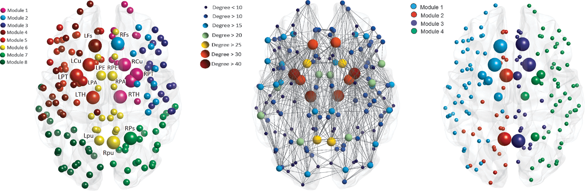
General structure of the average network. Left: decomposition into modules of the average network (Tc=0.0005, T _avg=75%). Different colors are associated to the eight different modules. Large-sized nodes are connector hubs and medium-sized nodes are provincial hubs specific to this decomposition. Center: Average network (Tc=0.0005, T _avg=75%) with size and colors of nodes depending on the degree. For clarity, only edges with strength over the mean strength are shown (unweighted). Right: decomposition into modules of the binary average network (Tc=0.0005, T _avg=75%). Different colors are associated to the four different modules. Large-sized nodes are connector hubs and medium-sized nodes are provincial hubs specific to this decomposition. Labels and names of the ROIs can be found in Supplementary Table S1. ROIs, regions of interest; T _avg, average network threshold; Tc, threshold connectivity.

Table 2.

Statistics of Global Network Metrics

	Average network (Tc=0.0005, T_avg =75%)		Individual networks (mean±SD)(Tc=0.0005)		Individual networks (mean±SD)(Tc=0.0005, TD=12.23%)		Random networks (mean±SD)(Tc=0.0005)
	Binary	Weighted	Binary	Weighted	Binary	Weighted	Binary	Weighted
Deg/S^w	14.34	0.33	23.03±3.12	0.34±0.06	18.71^*	0.34±0.06^*	23.03±3.12	0.34±0.06
CC	0.60	0.03	0.60±0.02	(1.0±0.3)×10⁻²	0.58±0.01^*	(1.4±0.3)×10⁻² ^*	0.24±0.03	(2.5±0.5)×10⁻³
L	2.41	99.00	2.14±0.08	101.6±16.7	2.31±0.04^*	101.6±16.7	1.89±0.04	65.1±10.3
Eff	0.47	1.36×10⁻²	0.53±0.02	(1.4±0.2)×10⁻²	0.49±0.01^*	(1.4±0.2)×10⁻²	0.57±0.01	(1.4±0.2)×10⁻²
Loc. Eff	0.80	0.03	0.80±0.01	(2.5±0.4)×10⁻²	0.79±0.01^*	(2.8±0.5)×10⁻² ^*	0.54±0.05	(7.8±2.2)×10⁻³
SW	3.01	3.02	2.22±0.21	2.61±0.28	2.54±0.15^*	2.88±0.24^*
Ax	−0.09	0.26	−0.06±0.02	0.31±0.09	−0.03±0.03^*	0.31±0.09^*	−0.13±0.02	0.04±0.05
Mod	0.47	0.66	0.42±0.02	0.65±0.02	0.44±0.03^*	0.65±0.02^*	0.15±0.09	0.46±0.01

Global metrics of the average network (Tc=0.0005 and T _avg=75%), the individual networks (Tc=0.0005, Tc=0.0005 with TD=12.23%), and the associated random networks (Tc=0.0005). Random networks are computed as in (Maslov and Sneppen, 2002) and more details can be found in see the section Graph metrics definitions in the Supplementary Material.

Significance of the paired test for values of global metrics with/without TD (p<0.05, corrected).

Ax, assortativity; CC, clustering coefficient; Deg/S^w, degree/strength; Eff, efficiency; L, characteristic path length; LocEff, local efficiency; Mod, modularity; SW, small-world property; Tc, threshold on connectivity maps; TD, density threshold; T _avg, average network threshold.

Variability in the average network

In order to evaluate the effects of variability between measurements on the average network, two average networks were created by random allocation of sessions to one of the two networks (see the section Quantification of reproducibility).

Variability of global properties

The percent difference of global measures (Supplementary Table S2) between the two networks was of 2% on average (over all T _avg and Tc). The highest percent difference was found for Ax with 9% on average over all thresholds.

Variability of local properties

For the variability of local properties, the Bland–Altman plot was considered. Results showed a tendency of larger errors for larger metrics values for weighted clustering coefficient (CC^w), CC, S^w, Deg, and weighted average node distance (NDist^w). This effect was stronger for CC^w and NDist^w (Fig. 2, left).

FIG. 2.

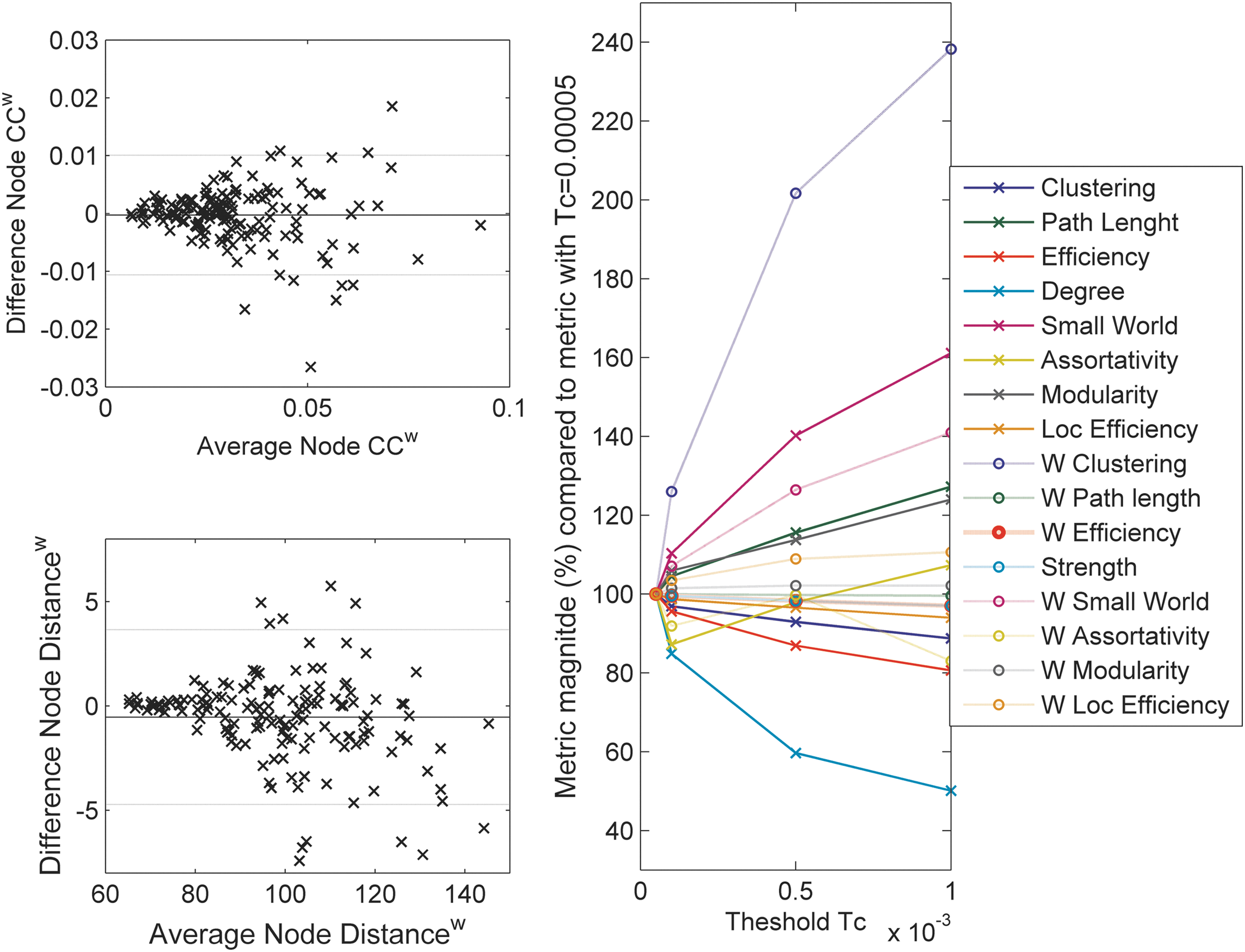
Left: variability of local network metrics of the average network. Bland–Altman plots for the node properties (CC^w [top] and NDist^w [bottom]) of the two average networks. Right: dependency of global metrics of the average network on threshold Tc. Plot of the ratio of global metrics with increasing threshold Tc over the metrics with lowest Tc (average network with T _avg=75%). CC^w, weighted clustering coefficient; NDist^w, weighted average node distance.

Effects of thresholds T _avg and Tc

The effect of Tc on the global properties of the average network is reported in Figure 2 (right). For most of the metrics the maximal change was of 20–30% as compared with the value with minimal Tc, but for CC^w there was an increase of 140% and for Deg there was a reduction of 60%. Also for the threshold T _avg, the largest effect was seen on Deg and CC^w. The percent change between measurements was not significantly different for different Tc and T _avg (Supplementary Table S2; one-way rANOVA T _avg: p<0.35 and Tc: p<0.43). The RI for the comparison of the partition into modules to the one for T _avg=75% and Tc=0.0005 (Fig. 1, left) was between 0.93 and 0.98. Overall, RI was higher for higher threshold T _avg and Tc.

Unthresholded individual networks

Networks in which TD was not applied are denoted as unthresholded and were analyzed to investigate the effect of setting a common density threshold on the networks. The analyses were completed for all Tc levels, and the obtained results were similar. Therefore, when the effect of Tc was not the focus of the analysis, results are reported for Tc=0.0005 only.

Similarity analysis: unthresholded connectivity matrices and modules

Weighted similarity within subject (WS; 0.97±0.02) was higher than BS (0.78±0.05), and the similarity between individual networks and average network was in between the two (0.89±0.02). A similar situation was found for the RI quantifying the similarity in the modules (Fig. 3, top).

FIG. 3.

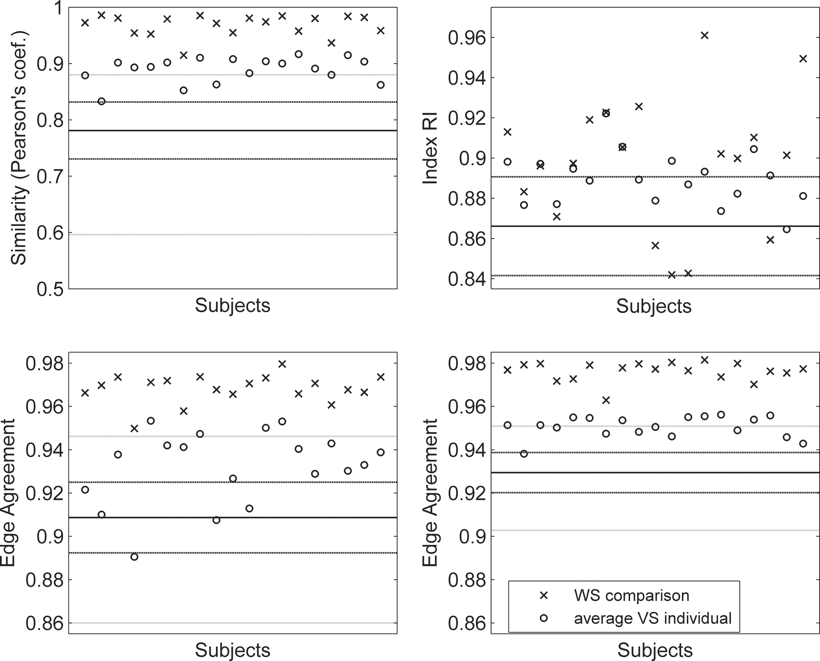
Top left: similarity of individual networks (Tc=0.0005) WS and compared with the average network. The central line indicates the average BS similarity. The narrow interval is given by±SD and the large interval indicates the range of BS similarity. Top right: similarity of decompositions into modules WS and compared with the average network (Tc=0.0005). The central line indicates the average BS RI and the interval±SD. Bottom: edge agreement of individual networks WS and compared with the average network. The central line indicates the average BS similarity. The narrow interval is given by±SD and the large interval indicates the range of BS similarity. Left: individual networks with Tc=0.0005. Right: individual networks with Tc=0.0005 and TD_max=12.23%. BS, between-subject; RI, Rand index; SD, standard deviation; TD_max, maximum common density; WS, within-subject.

Analysis of global metrics

Statistics of the global properties of the unthresholded networks are reported in Table 2.

Repeatability of global metrics for Tc=0.0005

The average absolute ICC and CV values over all properties were, respectively, of 0.86±0.11 and 4.27±4.39% (Table 3). The CV values were higher for weighted than for binary metrics (p<0.001), while the ICC values were slightly lower (p<0.002).

Table 3.

Repeatability Coefficients of Global Metrics

	Networks Tc=0.0005		Networks averaged over Tc		Networks Tc=0.0005, TD_max=12.23%		Networks Tc=0.0005, average over TD
Global metrics	ICC	CV	ICC	CV	ICC	CV	ICC	CV
CC	0.93	0.95	0.93	0.82	0.80	0.79	0.82	0.95
L	0.89	1.04	0.91	0.97	0.86	0.57	0.82	0.68
Eff	0.89	0.94	0.91	0.88	0.92	0.33	0.89	0.42
Deg	0.90	2.90	0.90	2.89
SW	0.92	2.30	0.94	1.89	0.95	1.09	0.85	1.48
Ax	0.81	−16.33	0.79	−16.26	0.84	73.79	0.87	−45.92
Mod	0.91	1.44	0.88	1.95	0.66	2.22	0.63	2.46
LocEff	0.92	0.38	0.93	0.33	0.73	0.32	0.75	0.53
CC^w	0.61	11.36	0.56	11.81	0.68	7.75	0.66	8.31
L^w	0.89	4.57	0.89	4.58	0.89	4.58	0.89	4.58
Eff^w	0.89	4.13	0.89	4.13	0.89	4.13	0.89	4.13
S^w	0.87	4.39	0.87	4.39	0.87	4.34	0.87	4.28
SW^w	0.91	2.86	0.90	2.89	0.90	2.08	0.81	2.76
Ax^w	0.88	9.06	0.88	9.05	0.88	9.09	0.88	9.04
Mod^w	0.56	1.77	0.55	1.77	0.47	1.84	0.40	1.72
LocEff^w	0.90	3.58	0.90	3.64	0.91	4.18	0.90	4.41
Average	0.86	4.25	0.85	4.27	0.82	7.81	0.80	6.11

Repeatability coefficients of global metrics with different thresholds Tc and TD.

Ax^w, weighted assortativity; CC^w, weighted clustering coefficient; Eff^w, weighted efficiency; LocEff^w, weighted local efficiency; Mod^w, weighted modularity; SW^w, weighted small-world property.

Effects of threshold Tc

In general, values of ICC and CV were not strongly affected by threshold Tc (Fig. 4; one-way rANOVA ICC: p<0.21 and CV: p<0.14), although with higher thresholds the ICC of Mod was decreased and the CV value (absolute) of Ax was increased.

FIG. 4.

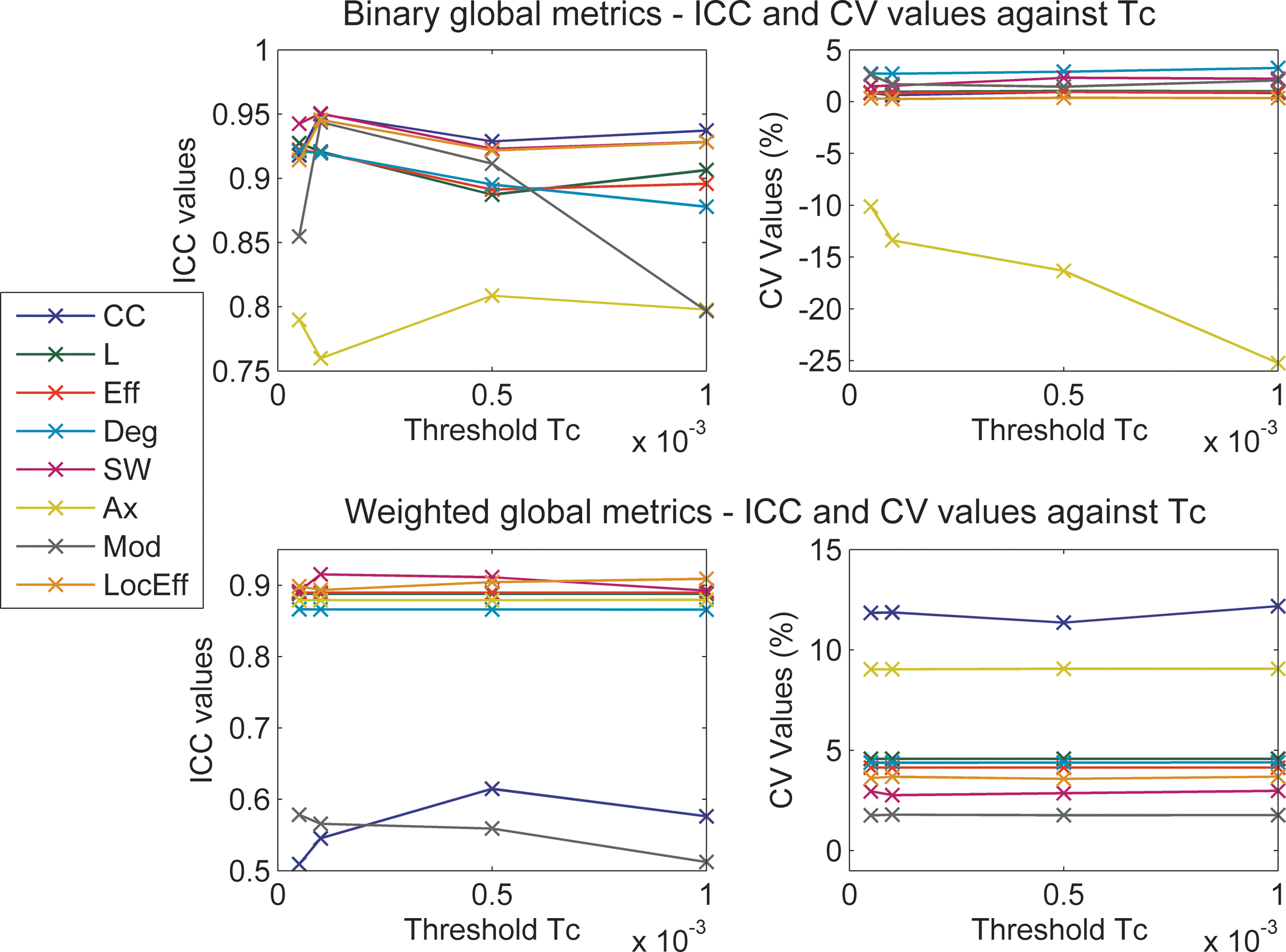
Dependency of global network metrics on the level of threshold Tc. Left: ICC values of global metrics against the threshold Tc for binary (top) and weighted (bottom) metrics. Right: CV values of metrics against the threshold Tc for binary (top) and weighted (bottom) metrics. CV, coefficient of variation; ICC, intraclass correlation coefficient.

Analysis of local metrics

A summary of statistics for local metrics of unthresholded networks is given in Table 4 for Tc=0.0005 and in Supplementary Table S3 for all Tc.

Table 4.

Statistics of Local Network Metrics

	Networks Tc=0.0005			Networks Tc=0.0005, TD=12.23%
	Value	ICC	CV	Value	ICC	CV
NDist	2.1±0.2	0.76±0.14^*	2.3±0.6^*	2.3±0.3^***	0.73±0.14^**	2.1±0.7^**
Deg	23.0±11.3	0.82±0.12^*	8.7±3.1^*	18.7±9.5^***	0.79±0.11^**	8.1±2.9^**
CC	0.60±0.12	0.75±0.13^*	5.2±1.1^*	0.58±0.13^***	0.74±0.13	5.4±1.3
LocEff	(5.2±0.4)×10⁻³	0.75±0.14^*	2.0±0.6^*	(5.0±0.4)×10⁻³ ^***	0.73±0.13	2.1±0.6^**
BC	174±402	0.67±0.20^*	32.0±11.1^*	200±462^***	0.66±0.19	33.2±125
NDist^w	101.0±17.5	0.85±0.06	5.6±1.2	101.0±17.5	0.86±0.06	5.6±1.2
S^w	0.34±0.22	0.80±0.12	9.9±3.0	0.34±0.22^***	0.80±0.12	9.9±3.1
CC^w	(10.0±4.0)×10⁻³	0.65±0.15	17.1±3.6	(14.0±6.0)×10⁻³ ^***	0.70±0.14^**	15.3±3.4^**
Loc Eff^w	(1.6±0.4)×10⁻⁴	0.79±0.11	9.0±2.5^*	(1.3±0.5)×10⁻⁴ ^***	0.78±0.12	9.9±2.9^**
BC^w	0.04±0.05	0.66±0.24	18.4±6.6	0.04±0.05	0.66±0.24	18.4±6.6

Local metrics values (mean±SD, averaged over subjects and nodes) and associated repeatability coefficients (mean±SD, averaged over nodes) of networks with Tc=0.0005 and, respectively, without TD or with TD=12.23%.

Repeatability coefficients that change significantly for different thresholds Tc (rANOVA, p<0.05 corrected). For details on the values see Table S3.

Repeatability coefficients that change significantly in the comparison with/without TD (paired test, p<0.05 corrected).

***

Average local metrics (over subjects) that change significantly in the comparison with/without TD (paired test, p<0.05 corrected).

BC, betweenness centrality; BC^w, weighted betweenness centrality; CV, coefficient of variation; ICC, intraclass correlation coefficient; NDist, average node distance; NDist^w, weighted average node distance; rANOVA, repeated-measures ANOVA.

Effects of threshold Tc

Tc had a significant effect on the value of all metrics except NDist^w and weighted betweenness centrality (BC^w). In addition, networks with lower Tc appeared to have slightly better local repeatability, although the effect was significant only for binary metrics and weighted local efficiency (LocEff^w) (Table S3 and Table 4). Overall, post hoc analyses showed that the differences were stronger for CV and for Tc=0.0005 against lower thresholds.

Local metrics repeatability for Tc=0.0005

Histograms of ICC and CV values of local properties are shown in Figure 5 for Tc=0.0005. ICC values were high on average, but locally low values were found. Overall, the CV values were higher than for global metrics and higher for weighted than for binary metrics.

FIG. 5.

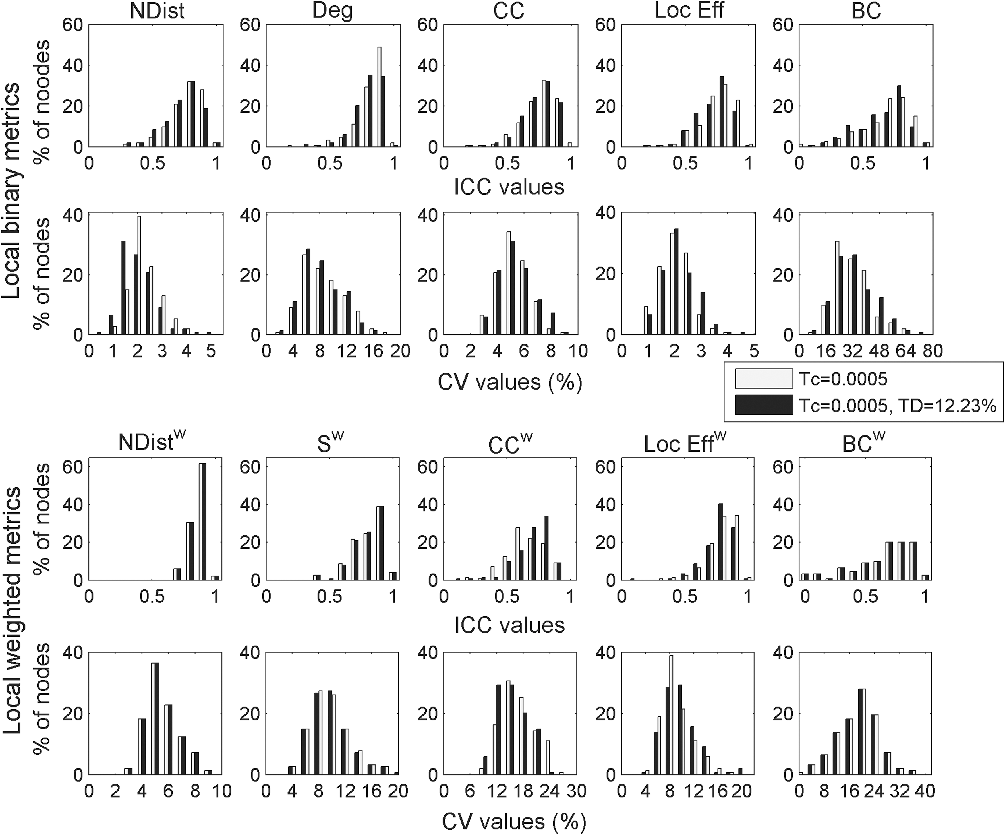
Evaluation of the repeatability (ICC, CV) of local network metrics and their dependency on threshold TD (with/without). Top (rows 1 and 2): Histograms of ICC and CV values of local unweighted metrics properties of networks with Tc=0.0005 (white bars) and networks with Tc=0.0005 and TD=12.23% (black bars). Bottom (rows 3 and 4): Histograms of ICC and CV values of local weighted metrics properties of networks with Tc=0.0005 (white bars) and networks with Tc=0.0005 and TD=12.23% (black bars). TD, density threshold.

Thresholded individual networks

In this section, the effect of a common density threshold (TD) on individual networks is considered. The analyses were completed for all levels of thresholds Tc and TD, and the obtained results were similar. Therefore, when the effect of different TD was not the focus of the analysis, results are reported only for Tc=0.0005 and TDmax=12.23%.

Similarity analysis, modules, and hubs classification

Similarity of thresholded connectivity matrices and modules

The similarity analysis of connectivity matrices and the decomposition into modules was very similar as for the unthresholded matrices. The median number of modules in the individual networks was 8 (range 5–13). When TD was applied, an increase of 1% to 3% in the edge agreement WS and BS was found (Fig. 3, bottom).

Hubs classification agreement

In Figure 6, the consistency of hubs classification in the individual networks is presented. On average (over hubs), in 87.4±17.1% of the subjects the hubs of the average network were classified as hubs. In 73.4±16.2% of the subjects the connector hubs of the average network were classified as connector hubs. The classification of provincial hubs was less consistent. In 61.4±3.0% of the subjects the provincial hubs of the average network (LPE, LPu, RPE) were classified as hubs, but only in 24.6±10.6% they were classified as provincial. The average hubs agreement WS was of 87.0±7.5% over all hubs. In addition, only for 47.0±37.6% of the subjects the same hubs were found also using S^w as a classification criterion, but the agreement was of 78.0±15.6% for the subcortical hubs. Other hubs using S^w were found in the insular and in the nucleus accumbens areas.

FIG. 6.

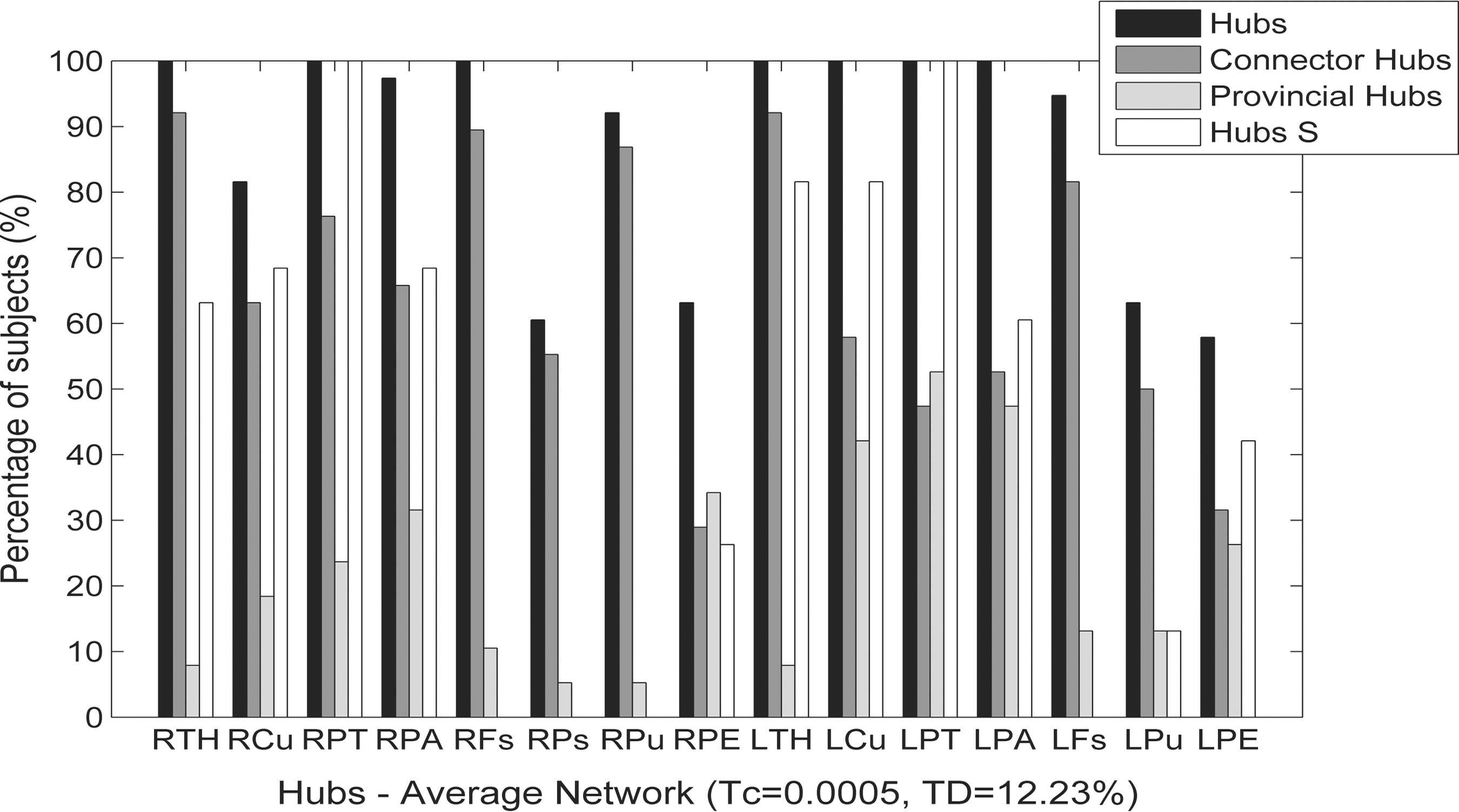
Evaluation of consistency of hubs classification in the individual networks. For each hub of the average network, the percentage of individual networks in which this node is also a hub is given. In addition, the percentage of subjects in which this hub is connector/provincial is given as well as the percentage of subjects in which this node is a hub defined with high strength (Hubs S).

Analysis of global metrics

Statistics of the global properties of these networks are reported in Table 2.

Effects of threshold TD value for Tc=0.0005

Differences with/without TD are significant for almost all metrics (Table 2). In general, the repeatability coefficients did not show a clear dependency on the threshold TD (Fig. 7, top), but for some of the metrics ICC values varied considerably for different TD (LocEff, modularity [Mod], weighted modularity [Mod^w], SW). For L, CC, Mod, Mod^w, and LocEff, results showed a reduction in the ICC (between 17% and 37%) by applying TD. For the other metrics the variation was always under 10%. Although CV values were small for binary metrics, they were decreased by 20% to over 200% by applying TD (except for Mod). For weighted metrics the variation was smaller.

FIG. 7.

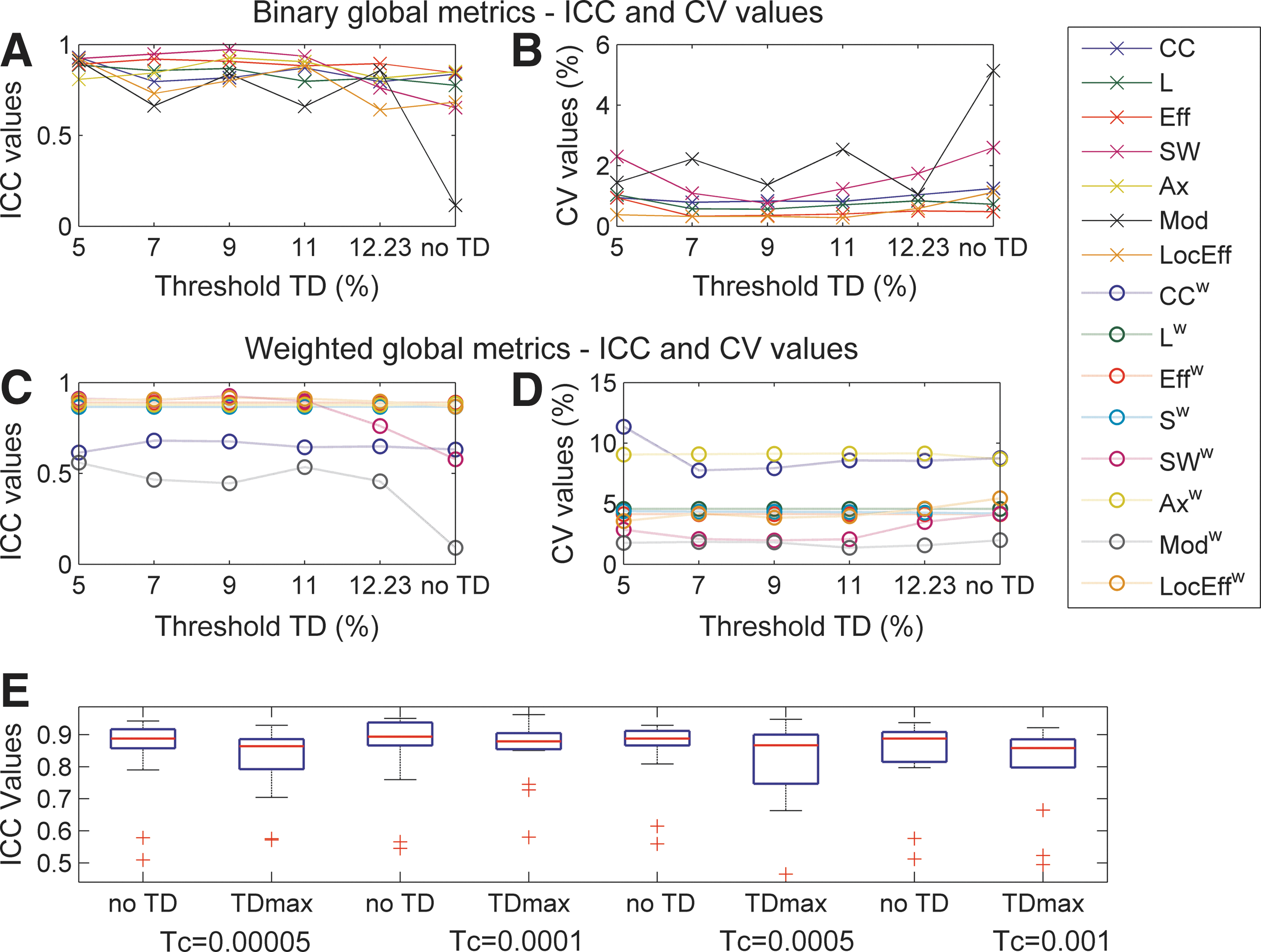
Evaluation of repeatability dependency on the level of threshold TD for global network metrics (CC, L, Eff, SW, Ax, Mod, and LocEff binary and weighted). Repeatability of the metrics is quantified by ICC and CV coefficients. ICC (A) and CV (B) values of binary global metrics against threshold TD. ICC (C) and CV (D) values of weighted global metrics against threshold TD. (E) Box plot of the ICC values of weighted and binary global metrics classified by the value of threshold Tc and the condition with/without TD. Ax, assortativity; CC, clustering coefficient; Eff, efficiency; L, characteristic path length; LocEff, local efficiency; Mod, modularity; SW, small-world property.

Effects of threshold TD for different Tc values

A two-way rANOVA including the levels of Tc and the condition with/without TD as repeated measures showed a significant effect on ICC values for Tc (p<0.018) and for the interaction (p<0.009; Fig. 7, bottom). However, in the post hoc analyses the comparison of the condition with/without TD for each threshold Tc was only near to significant. No significant effect was found on CV values.

Analysis of local metrics

Summary statistics for local metrics and their repeatability are given in Table 4 and histograms are shown in Figure 5.

Effects of threshold TD with Tc=0.0005

Applying TD had a significant effect on all local metrics except NDist^w and BC^w (Table 4). Except for CC^w, for these metrics a small reduction in ICC was found. Variations of CV are significant for most of the metrics but depend also on the changes of the metrics values.

Effects of ROI size

Correlations between values of local metrics (averaged over subjects), ROI size, and repeatability coefficients are reported in Table 5 (Fig. 8). Overall, results showed that smaller ROIs were associated with poorer repeatability (higher CV, lower ICC). However, correlations were significant only for CV values and some of the metrics considered, while the correlations coefficients between ROI size and ICC were small (Table 5). In order to investigate if the effect of ROI size on the CV values was only because of the relationship between the metrics values and CV (Fig. 8, top), a multiple linear regression including ROI size and metrics values as regressors was used for the CV of NDist, Deg, CC, LocEff, BC, S^w, CC^w, and LocEff^w. After correction, for most of the metrics, only the contribution of the metrics values was found to be significant. For S^w also the ROI size had a significant contribution (ROI: p<0.001), and for LocEff^w this effect was the only one significant (ROI: p<0.026, Val: p<0.232). For CC, NDist^w and BC^w significant linear relationships between the metric values and the ICC values were also found. For NDist^w (Fig. 8, bottom), two strong correlations indicate that higher values of NDist^w are associated with lower repeatability (ICC: r=−0.42, CV: r=0.47, Pearson's coeff).

FIG. 8.

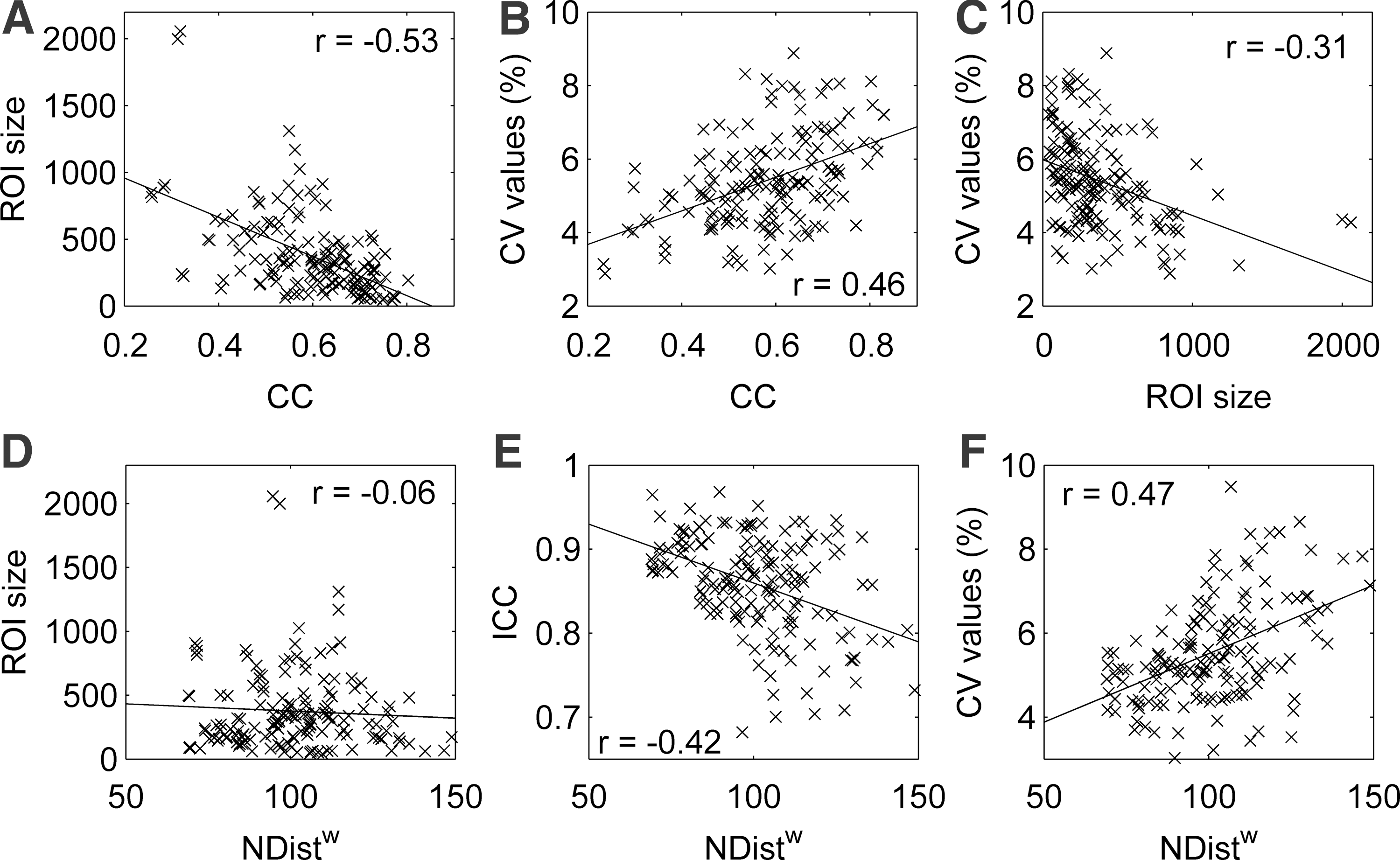
Evaluation of the relationship of two local metrics (CC, NDist^w), their repeatability coefficients, and the size of nodes (ROI size). Top row: the relationship between ROI size and CV values is linked to the dependency of CV on the metric values. Scatter plots: (A) local CC against ROI size (r=−0.53 Pearson's coef); (B) local CC against CV values (r=0.46 Pearson's coef); (C) ROI size against CV values of local CC (r=−0.38 Pearson's coef). Bottom row: strong correlations were found between local NDist^w and its repeatability coefficients. Scatter plots: (D) local NDist^w against ROI size (r=−0.06 Pearson's coef); (E) local NDist^w against ICC values (r=−0.42 Pearson's coef); (F) local NDist^w against CV values (r=0.47 Pearson's coef).

Table 5.

Correlations with ROI Size

	Value/ROI size	Value/ICC	Value/CV	ROI size/ICC	ROI size/CV
NDist	−0.48^*	−0.21^†	0.32^*	−0.07	−0.26^†
Deg	0.49^*	0.17^†	−0.53^*	0.01	−0.41^*
CC	−0.53^*	−0.33^*	0.46^*	0.11	−0.38^*
LocEff	−0.53^*	−0.26^†	0.58^*	0.08	−0.43^*
BC	0.39^*	0.20^†	−0.43^*	0.18^†	−0.45^*
NDist^w	−0.06	−0.42^*	0.47^*	0.09	−0.10
S^w	0.16^†	0.21^†	−0.32^*	0.05	−0.32^*
CC^w	−0.56^*	−0.06	0.33^*	0.06	−0.41^*
LocEff^w	−0.46^*	0.06	0.32^*	0.18	−0.37^*
BC^w	0.19^†	0.28^*	0.18^†	0.08	0.03

Correlations for local properties of networks with Tc=0.0005 and TD=12.23%. Correlations between local metrics values, ROI size, and variability coefficients.

Significant correlations (p<0.05 corrected).

†

Significant correlations (p<0.05 uncorrected).

Note: significance was not affected by the exclusion of the two outliers with larger size.

ROI, region of interest.

Analysis of connections repeatability

The relationship between connection strength, ROI size, and distance was analyzed in order to understand if there was any bias in the weights. For this analysis, the distance functions and the connection matrices were averaged over all subjects.

Relationship between weights, number of connections, and ROI size

In Figure 9A, a plot of the weights of the connections between nodes ordered according to the size is shown. There was no structure in the weights distribution, suggesting that no bias was present. However, there were a higher number of connections among larger nodes. In particular, there were 386 edges connecting the larger 50 ROIs, while only 171 edges between the 50 smaller ROIs.

FIG. 9.

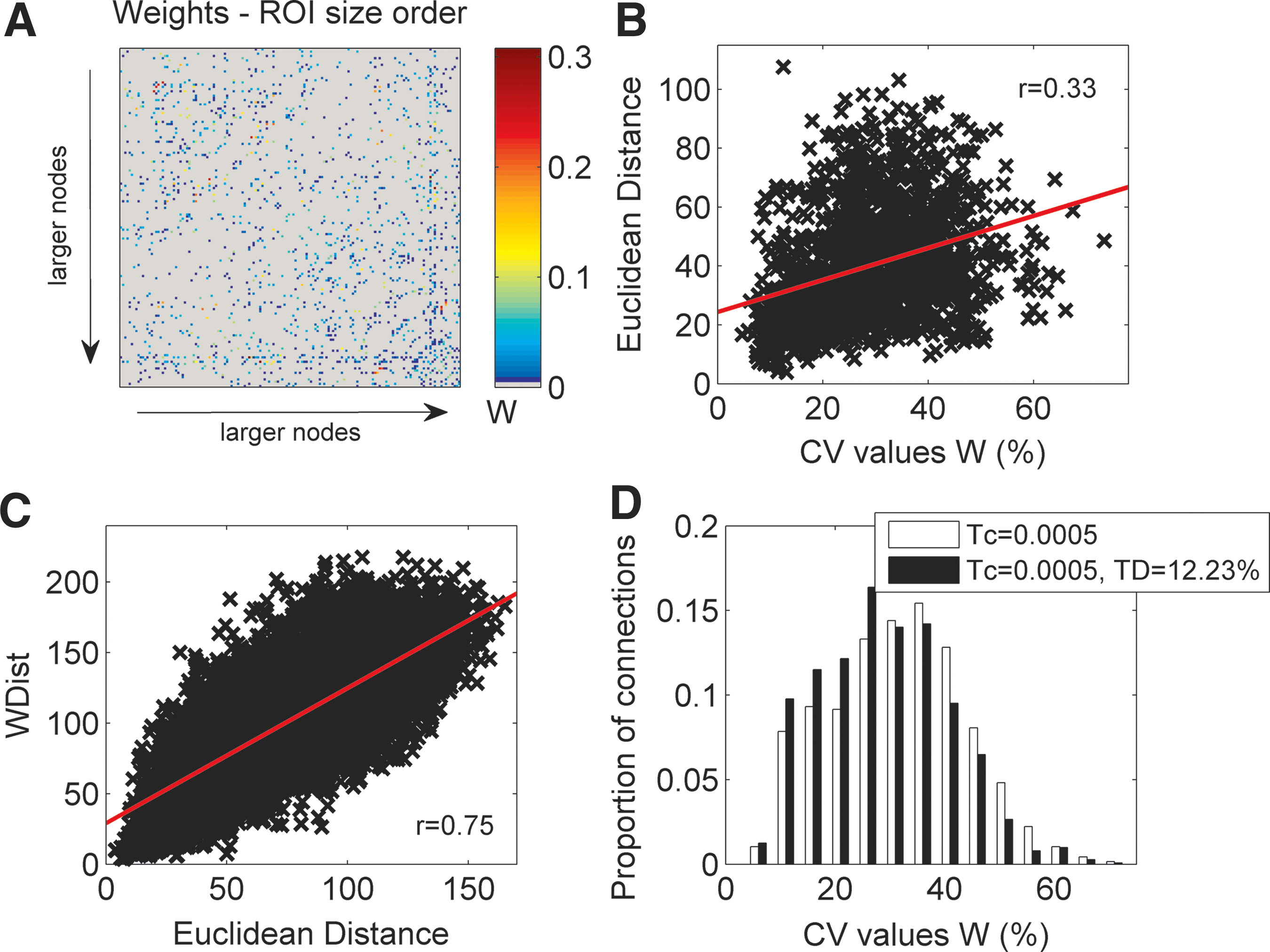
Analysis of the relationship between weights and ROI size and of the repeatability of specific connections. For these analyses, average matrices over all subjects were used. (A) Weights distribution for nodes ordered according to increasing ROI size. The color scale is associated to the connection weights. (B) Scatter plot of the Euclidean distance between connected ROIs against CV values of the related connections weights. (C) Scatter plot of Euclidean distance versus Dist^w indicating that physical distance and network distance are strongly related. (D) Histogram of average CV values of weights in networks with or without threshold TD.

Relationship between distance, connections weights, and repeatability

A negative correlation was found between connections weights and Euclidean distance of connected nodes (r=−0.44), while Euclidean distance and CV values of the weights were positively correlated (r=0.33; Fig. 9B). The first relation is known to be one of the drawbacks of probabilistic tractography, as the connection probability is reduced for longer connections (Jbabdi and Johansen-Berg, 2011). Euclidean distance strongly correlated with the distance functions of the network (Dist: r=0.64, Dist^w: r=0.75; Fig. 9C). In Figure 9D, CV values of the edges weights with and without threshold TD are shown. There was a slight shift toward lower values in thresholded networks.

Discussion

Structural brain networks of 19 healthy subjects were constructed for 2 consecutive measurements and were analyzed in the current study to assess three major questions: (1) the effects of between measurements variations on the average network of all subjects, (2) reproducibility of local network metrics, and, finally, (3) the effects of a common density threshold on the values and reproducibility of networks metrics. In addition, in the first part of the discussion our results are presented in relation to previous works in order to highlight replications.

Overview of the results: comparison with previous literature

A large set of global and local metrics was computed for the individual weighted and binary networks as well as for the average network. Overall, the network topology characteristics were in line with prior literature.

Consistently with previous studies, our network was decomposed into a central core module and some additional mostly symmetric hemispheric modules (Li et al., 2012; Owen et al., 2013), dividing each hemisphere into anterior and posterior and additionally dividing anterior nodes into a superior and a medial inferior module. The mean RI for the agreement of modules between the average network and the individual networks was approximately of 0.9, showing that these modules were quite consistent across subjects (Fig. 3).

Hubs were found in the subcortical regions of the thalamus, putamen, caudate, and pallidum and in the frontal superior and parietal superior cortex as well as in the precuneus and pericallosal areas (Fig. 1, left). The hubs regions are consistent with previous studies (Li et al., 2012; Owen et al., 2013; van den Heuvel and Sporns, 2011) in which subcortical nodes are considered. However, studies focusing on the cortical network only also consistently report regions of the insular and the cingulate cortex (van den Heuvel and Sporns, 2013), which in our case were only classified as hubs in some of the individual networks. In both cases, hubs of the brain structural network have been found to be highly connected, forming a rich-club that is crucially responsible for the global communication in the connectome (van den Heuvel and Sporns, 2011, 2013; van den Heuvel et al., 2012). Additionally, based on the network decomposition into modules, hubs can be classified into connector hubs, which have a role in the integration of the different modules, and provincial hubs, which are important for communication within a module (van den Heuvel and Sporns, 2011, 2013). In our analysis, more connector hubs were found than in van den Heuvel and Sporns (2011). This difference may be because of the finer parcellation used in our study, but more probably it is additionally related to the different decomposition with a large number of modules. Indeed, 8 modules including a central module were found in our analysis, while 4 modules with no inter-hemispheric module were found by van den Heuvel and Sporns (2011). The additional connector hubs found in the anterior modules were important for connections with the other frontal module of the same hemisphere (thalamus, pallidum, putamen) and with the symmetric module (caudate). Hubs of the average network were classified as hubs in most of the individual networks (approximately 90% on average; Fig. 6); however, this agreement was lower for the classification of connector and provincial hubs.

In the current study, repeatability of brain structural networks was tested over several levels: unthresholded connectivity matrices, global networks metrics, and local level (nodes and edges). Previous studies already considered various aspects of the first two levels, allowing for a comparison of our results with previous literature, while only limited results were presented for local metrics (Table 1) (Bassett et al., 2011; Buchanan et al., 2013; Cammoun et al., 2012; Cheng et al., 2012; Dennis et al., 2012b; Hagmann et al., 2008; Vaessen et al., 2010). A summary of previous results on similarity of connectivity matrices and ICC of global metrics is given in Table 6, in which all studies on the repeatability of global networks metrics to our knowledge were included. More details on the methodology of the studies are given in Table 1. Overall, our results indicated good to excellent repeatability (ICC>0.75 and CV<5%) of global measures and were more in line with the results of Owen and associates (2013) as compared with previous studies. Hence, our results confirm that global network metrics in healthy subjects are sufficiently reliable to be used as clinical biomarkers. This is one first step toward the use of these biomarkers for diagnosis, prognosis, and further understanding of specific neurological and psychiatric diseases, although in diseased populations reliability should be tested specifically as both segmentation and tractography poses more problems in damaged tissue (Budde et al., 2011; Fiez et al., 2000; Nakamura and Fisher, 2009; Pagani et al., 2005). The comparison of the different studies is difficult, because of the variability in various methodological aspects; nonetheless, it can highlight points that may be beneficial for repeatability of the network metrics. The agreement with the results of Owen and colleagues may be because of methodological similarities. In particular, in both studies DTI was preferred to high-angular-resolution diffusion imaging (HARDI) methods, allowing a short acquisition time for DWI (5.22 min per DTI sequence). Also, the atlas-based parcellation was performed in native space (FreeSurfer) avoiding errors because of coregistration of all subjects to a common space, and probabilistic tractography (FSL) was preferred. Probabilistic tractography adds an estimation of the propagation of local uncertainty, thus enabling to better explore possible complex fiber configurations and resulting in more robust results (Descoteaux et al., 2009; Moldrich et al., 2010; Tournier et al., 2011). Despite differences in other methodological aspects, in the comparison of our results and the ones of Owen and colleagues (2013) against previous studies using deterministic tractography and white matter (WM) seeding (Bassett et al., 2011; Cheng et al., 2012), repeatability of global network metrics seems to benefit of the use of probabilistic tractography. In particular, studies using deterministic tractography report similar values for the CV, but lower ICC values (mostly under 0.65; see Table 6). This result also holds when including all previous studies using probabilistic tractography in the comparison. For local strength, a direct comparison was presented in the study of Buchanan and associates (2013), which confirms this result. Nevertheless, in the same study the authors show that WM seeding improves repeatability and has a stronger impact than the tractography algorithm. The benefit of WM seeding is, however, not supported by our comparison of previous literature. General advantages and drawbacks of probabilistic tractography and associated weighting schemes are discussed further in the Limitations section. Finally, the same weighting scheme was used for weighted metrics in our study and the one of Owen and colleagues. This scheme was shown to provide better local repeatability compared with similar weights additionally corrected for the connection length (Buchanan et al., 2013). All these methodological similarities may be beneficial for repeatability and explain the differences from prior works where only moderate to good repeatability was found (Owen et al., 2013).

Table 6.

Comparison with the Previous Literature

	Similarity		ICC
Study	WS	BS	Deg/Dens	L	CC	SW	Eff	BC	LocEff	Ax	S	Mod
Vaessen and associates (2010)			0.63	0.64	0.48
Bassett and colleagues (2011)
DTI	0.93	0.82	0.65	0.53	0.45		0.37	0.28	0.42	0.40	0.93	0.21
DSI	0.97	0.95	0.25	0.45	0.2		0.32	0.32	0.21	0.31	0.72	0.09
Cheng and associates (2012)
W1	0.89	0.72		0.44	0.64	0.59	0.30					0.47
W2	0.84	0.66		0.28	0.54	0.55	0.64					0.67
Owen and associates (2013)
Binary	0.96	0.93	0.79	0.92	0.51		0.92	0.90	0.54
Weighted	0.96	0.92		0.67	0.83			0.50			0.84	0.56
Dennis and associates (2012)				0.59	0.58	0.52	0.59
Buchanan and colleagues (2013)			0.66	0.62	0.76						0.75
Analysis
Binary	0.98	0.93	0.90	0.86	0.80	0.95	0.92		0.73	0.84		0.66
Weighted	0.97	0.78		0.89	0.68	0.90	0.87		0.91	0.88	0.87	0.47

Summary of previous results on the repeatability of connectivity matrices and global metrics (ICC). Some of the values are averaged over different modalities or estimated from figures. For our analysis, results reported are with Tc=0.0005 and TD=12.23% (except for Deg). Additional information on the studies is reported in Table 1.

However, the two studies differ in the atlas used: Owen and colleagues used “Desikan-Killiany” FreeSurfer atlas (Desikan et al., 2006), while in our analysis the finer parcellation of “Destrieux” FreeSurfer atlas was used (Fischl et al., 2004). The choice of the atlas defining the nodes as well as the node sizes has been previously shown to have an effect on the network metrics values (Bassett et al., 2011; Zalesky et al., 2010). In the comparison of repeatability with different atlases and resolutions, Bassett and colleagues (2011) reported a significant effect of both with higher repeatability for weighted global network metrics at higher resolution scales. Hence, our finer parcellation may also contribute to increased repeatability compared with previous works. However, Cammoun and associates (2012) found lower similarity in connectivity networks with higher resolutions, and also our results on the relationship of node size and repeatability suggest that at the local level the effects of noise are more evident for smaller nodes (see the section Repeatability of local properties).

Overall, the comparison of our analysis with previous literature highlights that, although quantification may be very sensitive to methodological characteristics such as the acquisition method, the parcellation atlas, and the resolution, consistent results on the brain structural network topology are found in the literature (i.e., hubs positions, modular structure, small-world properties, etc.). This suggests that network analyses are robust to a certain level of variations in the methodological pipeline. However, replications of results in repeatability of networks metrics are very important exactly because a large variability in methodological characteristics exists (Table 1) and previous studies are not sufficient to conclude on how results on repeatability can be generalized for different methodological choices. In previous studies, overall less than 100 subjects were included and differences exist in the acquisition method, the maximal b-value, the tractography algorithm, the parcellation scheme, the weighting scheme, and the thresholds applied (Table 1). All these characteristics can influence the quality of the analysis and therefore replications of studies on repeatability covering all the methodological possibilities are necessary.

The average network

Only edges that are consistent over a large number of the networks (T _avg=65–85%) are included in the average network. Therefore, it should represent the core of the individual networks that is mostly consistent over the population. Indeed, similarity between average and individual networks is higher than BS. In our analysis the average network (with Tc=0.0005 and T _avg=75%) had a density around 15%, and considering the differences in number of nodes, its metrics were in agreement with the results of Sporns and colleagues (2007).

In order to evaluate the effects of variability between measurements on the average network, two different networks were constructed, each using one of the measurements of each subject. For global metrics, results showed percent differences on average of 2%. These variations were in the same range of the CV values of individual networks. For some local metrics, the Bland–Altman plots revealed a relationship between the value of the metrics and the errors. In particular, larger errors were associated to longer average node distance (NDist^w). This result suggests that longer connections were more difficult to reconstruct.

In summary, the variability of the average network because of different measurements reflected in a straightforward way the results found for the individual networks.

Recently, de Reus and van den Heuvel (2013a) proposed a method to estimate false positives and negatives in group networks depending on threshold T _avg. They concluded that with thresholds in the range of 30–90%, similar levels in the elimination of false positives and negatives are obtained. These results suggest that the variability of the average network will be similar in this range, which is consistent with our results (Supplementary Table S2). The thresholds selected in our study are in the higher part of this range, reducing the number of false positives. This is a reasonable choice, as de Reus and van den Heuvel (2013a) used deterministic tractography and the number of false positive is probably higher with probabilistic tractography (Moldrich et al., 2010). Although the network metrics reported are mostly different, our results concerning the effect of T _avg on the network metrics value also are in line with the results of de Reus and van den Heuvel (2013a).

Repeatability of local properties

Local repeatability was analyzed at the nodes and the edges level and overall larger variability was found as compared with the global metrics. While for the ICC low values (ICC<0.5) were only a minority, CV values were on average of over 10% over all local metrics and higher for weighted metrics. CV values for edges weights were on average of approximately 30%. While the ICC is related to the sensitivity of the metric to BS differences, the CV is an estimate of the precision of the metric within subject. Therefore, metrics with high ICC and also relatively high CV are sensitive to individual variability, but not very precise (Owen et al., 2013). This analysis shows that although repeatability of global metrics is from good to excellent, at the local level there is substantially more variability. Global metrics are mostly defined as the average over nodes of a local metric and this suggests that the averaging corrects for the variability that is present locally. Also, it is not surprising that local repeatability is quite variable, as it is known that tractography is more difficult in specific tracts configurations (Jbabdi and Johansen-Berg, 2011; Jones et al., 2013). Additionally, on the neurobiological point of view, more variability is expected at the local level. Indeed, healthy brain structural networks are expected to be similarly organized, but with locally different patterns of connectivity specific to each individual (Bassett et al., 2011; Cammoun et al., 2012; Cheng et al., 2012). Overall, our results generalize to a larger set of binary and weighted metrics the results presented in prior works (Bassett et al., 2011; Buchanan et al., 2013; Owen et al., 2013; Vaessen et al., 2010). This information should be considered in (longitudinal) analyses at the local level. In particular, poor to moderate repeatability was found for BC, which was previously used also to classify nodes and define hubs (Li et al., 2012). However, our results on hubs consistency suggest that defining the hubs based on high degree is a robust method and high consistency is found within subjects (87.0±7.5%). Probably this is because the degree distribution is long-tailed (see Supplementary Fig. S1 or Owen et al., 2013), so that, despite variability, hubs still have considerably higher degree than the other nodes. Furthermore, in the present study efforts were put in understanding whether some regions were more prone to systematic lower repeatability than others, but no strong local dependency on the reliability level was found (unshown analysis). However, considering the nodes with lower repeatability for all metrics (Supplementary Table S4), some regions were found to have lower repeatability (higher CV or lower ICC) in both hemispheres and for more than one metric. With these criteria, the less reliable regions were found in orbital and temporal lateral regions, pre- and post-central regions, as well as in the occipital superior and transversal region.

In the literature, two approaches are more commonly used to define nodes. On one side, nodes can be defined using anatomical regions defined by an atlas. On the other side, some authors use a larger number of regions of the same size, not strictly related to an anatomical structure (Bassett et al., 2011; de Reus and van den Heuvel, 2013b; Hagmann et al., 2008; Owen et al., 2013; Zalesky et al., 2010). In the present work, the first option was preferred and the relationship between ROI size, local metrics, and node repeatability coefficients was analyzed in order to understand the effect of having different-sized nodes. The analysis showed strong relationships between most of the metrics and the ROI size. This effect is likely to depend on the relationship between degree and ROI size. Clearly, a large region has more distinct connections than a smaller region and the degree affects (by definition) many of the scalar metrics considered. Moreover, in the analysis of edges repeatability, no bias was found indicating higher weights for connections linked to larger nodes (Fig. 9A) (consistent with Cheng et al., 2012). These results together suggest that the selected weighting scheme allows correcting for bias in the edge weight magnitude, but cannot correct for the fact that larger ROIs are more likely to have a larger number of connections. This is a drawback of parcellations related to specific brain atlases, which could be improved by subdividing larger regions in order to have regions with similar size. On the other side, the analysis also showed that metrics of larger nodes were more precise (lower CV). Although this result is also related to the relationship between metric value and ROI size, it suggests that an excessive subparcellation will reduce reliability (Buchanan et al., 2013; Zalesky et al., 2010). Additionally, in line with this idea lower repeatability of local strength (see the Supplementary Material in Bassett et al., 2011) and lower similarity (Cammoun et al., 2012) were found at higher resolutions.

Another interesting result at the local level was that weighted average node distance was not related to the node size, but it was related to both its repeatability coefficients. In particular, nodes with higher average distance had poorer repeatability, suggesting that longer connections are less reproducible. This result is consistent with the repeatability analysis of the average network and also with results on single connections. Indeed, for single direct connections, a positive association was found between CV and the Euclidean distance between the connected nodes (Fig. 9B). All these results suggest that longer tracts are less reproducible and are consistent with the analysis of Owen and associates (2013).

Effects of a common density threshold on repeatability

Two different thresholds were applied on the individual networks. First, a threshold was set on the minimal connectivity index used to define edges. The connectivity index relates to the probability that a connection exists; hence, the threshold Tc exclude connections with low probability as they are likely to be false positives. Additionally, a common density threshold (TD) on all the individual networks was applied, because network metrics are affected by the number of edges and nodes, and hence network metrics are better comparable for networks with the same density (Anderson et al., 1999; Bassett et al., 2011; Stam et al., 2007; van Wijk et al., 2010). However, it may be argued that applying TD real differences across subjects may be eliminated and that differences in the density of brain networks of healthy subjects (with the same number of nodes) are not large enough to significantly affect the network organization properties (Buchanan et al., 2013; Owen et al., 2013). The methodological choice of applying or not applying a threshold on the density was shown to have a significant effect on the values of almost all the metrics considered. In our analysis, also the effects on the repeatability coefficients of applying TD were considered. At the global level, the variations in repeatability coefficients were small, although the ICC coefficients were overall slightly reduced when TD was applied. Similar results were found at the local level. As many networks metrics depend on the degree, it is not surprising that fixing the density, the variability is reduced. The ICC depends on both the WS and BS variability and a reduced ICC indicates that the BS variability reduction is more important. In addition, with threshold TD the edge agreement of the connectivity matrices was significantly increased BS and WS (Fig. 3). This suggests that applying TD, not only the number of edges is the same for all subjects, but also the binary networks compared are more similar; that is, the connections considered are mostly the same for all subjects. Hence, our results suggest that when TD is not applied, first, the values of network metrics change significantly, and second, differences in (binary) metrics are slightly inflated by the differences in density and this can have an effect on the ICC values. However, despite the fact that the excluded connections had very small weights and that similarity was increased (both WS and BS) by applying TD, our analysis is not sufficient to determine whether the differences in the overall connectivity BS are because of noise or if they are real. Therefore, these differences should be analyzed as a first step since they may be an important result in itself. Further on, a robust approach could be to consider both thresholded and unthresholded networks to better evaluate the effects of differences in density on the network topology. This approach was previously suggested by van Wijk and colleagues (2010); in the same article, the authors discuss different methods to compare network metrics. Also, differences in network metrics and in total connectivity (density) should be interpreted in relationship to the clinical question of interest. Finally, it was found that weighted metrics are less affected by the application of different thresholds (TD and Tc) as low weights have lower influence. Therefore, although the choice of an unbiased weighting scheme that represents true connectivity remains an open issue in brain structural networks analysis (Iturria-Medina et al., 2007; Jbabdi and Johansen-Berg, 2011; Meskaldji et al., 2013), weighted measures may have the advantage of not requiring setting thresholds.

Limitations

In the present study, probabilistic tractography was preferred over deterministic tractography despite the higher computational requirements of this method. Our analyses were not sufficient to compare directly probabilistic and deterministic tractography algorithms and our preference was based on previous literature (Buchanan et al., 2013; Descoteaux et al., 2009; Moldrich et al., 2010; Tournier et al., 2011). Also, alternative solutions (Mangin et al., 2013) such as global tractography were so far never used in the literature in the context of test–retest of network metrics; hence, it was infeasible to evaluate these techniques. Probabilistic tractography adds a component of uncertainty in the tracking, which may be beneficial to reconstruct complex fiber configurations, but also increases the number of false positives (Moldrich et al., 2010). In addition, introducing this uncertainty component offers a natural way of quantifying the confidence in the existence of a specific tract. This characteristic helps determining spurious connections, but it may be misleading in the interpretation of the weights arising from tractography results (Jbabdi and Johansen-Berg, 2011; Jones et al., 2013). Indeed, such weights will include the effect of relevant characteristic of the WM fiber tract such as the fiber density or the myelination as this influence the diffusion properties. However, such effects are indirect and difficult to characterize and weights will also be affected by the measurement noise, fiber tract shape, and length. Moreover, the tractography algorithm may introduce some asymmetry in the connectivity indices, indicating that a connection from A to B is more probable than a connection from B to A. Asymmetry is not present in diffusion data and, in our analysis, asymmetry arising from the tractography is prevented by making the connectivity matrix symmetric (see Methods: Data Processing).

Despite the difficulties in correctly interpreting the weights, weighted metrics were assessed and analyzed as they recently become more frequent in the literature [e.g., Buchanan and associates (2013), Ivkovic and colleagues (2012), and van den Heuvel and Sporns (2011)]. However, only one weighting scheme was considered in the analysis. The selected weighting scheme is one of the most commonly used in the literature (Cheng et al., 2012; Iturria-Medina et al., 2007, 2011; Owen et al., 2013; van den Heuvel and Sporns, 2011). Questions on how different weights influence the networks topology and/or the repeatability coefficients and questions on how weights could be improved to reflect true connectivity are important and interesting issues in this field, but were out of the scope of this article. In a similar way, many methodological characteristics (acquisition method, tractography algorithm, parcellation method, and atlas) that could affect the network metrics were fixed in our analysis. Differences in global metrics repeatability because of variations in most of these methodological characteristics were previously investigated (Bassett et al., 2011; Cheng et al., 2012; Vaessen et al., 2010), and therefore we decided to select methodologies commonly used in the literature and to focus on other questions.

Finally, a limitation exists in the comparison of our results to previous repeatability analyses because in our study DWI measurements were consecutive, while in previous studies measurements were taken on different days. This difference is not greater than other methodological differences between the studies but may possibly slightly decrease WS variability. Indeed, as our subjects stay in the scanner for the two measurements, coregistration will be similar for both datasets, limiting differences in this step of the procedure. In our analysis, the WS similarity of connectivity matrices is higher than BS similarity (Fig. 3, top). Although this result is in line with previous studies, the gap between the two is higher in our analysis (Table 6), which is in line with our hypothesis of increased WS similarity. On the other side, this methodological difference can provide insights in the contribution of distinct positioning on the reliability of the reconstructed networks.

Conclusion

The current study presents a test–retest analysis of structural brain networks and related global and local metrics. In line with previous research, reproducibility of global metrics was good to excellent (ICC>0.75 and CV<5%), confirming that global metrics in healthy subjects are sufficiently reliable to characterize the brain structural network in the healthy population and be used as reference for comparison with subjects affected by specific neurologic and psychiatric diseases. However, for local metrics more variability with locally poor reproducibility was found, and longer tracts were less reproducible than shorter ones. Moreover, the variability in the average network reflects in a straightforward way these results. By applying a threshold on the density, not only is the number of edges the same for all subjects, but also the binary networks compared are more similar. In addition, results showed that such methodological characteristics may affect the network metrics and their repeatability. Hence, the meaning and effect of each threshold should be understood, and differences in global connectivity as well as in the metrics should be interpreted in relationship to the clinical question explored as well as to the methodological pipeline applied. Despite the difficulties in comparing previous literature, the summary analysis of our results and previous studies on network metrics repeatability enabled to discuss the benefits and role of some methodological characteristics. Overall, our findings add useful information to future studies on brain networks that include longitudinal analyses or group comparisons and certainly suggest points that should be tested more specifically in the future.

Footnotes

Author Disclosure Statement

No competing financial interests exist for any of the authors of this article.

References

Anderson

, Butts

, Carley

. 1999. The interaction of size and density with graph-level indices. Soc Netw, 21:239–267.

Bassett

, Brown

, Deshpande

, Carlson

, Grafton

. 2011. Conserved and variable architecture of human white matter connectivity. Neuroimage, 54:1262–1279.

Behrens

, Woolrich

, Jenkinson

, Johansen-Berg

, Nunes

, Clare

, Matthews

, Brady

, Smith

. 2003. Characterization and propagation of uncertainty in diffusion-weighted MR imaging. Magn Reson Med, 50:1077–1088.

Bernhardt

, Chen

, He

, Evans

, Bernasconi

. 2011. Graph-theoretical analysis reveals disrupted small-world organization of cortical thickness correlation networks in temporal lobe epilepsy. Cereb Cortex, 21:2147–2157.

Buchanan

, Pernet

, Gorgolewski

, Storkey

, Bastin

. 2013. Test-retest reliability of structural brain networks from diffusion MRI. Neuroimage, 86:231–243.

Budde

, Janes

, Gold

, Turtzo

, Frank

. 2011. The contribution of gliosis to diffusion tensor anisotropy and tractography following traumatic brain injury: validation in the rat using Fourier analysis of stained tissue sections. Brain, 134:2248–2260.

Bullmore

, Sporns

. 2009. Complex brain networks: graph theoretical analysis of structural and functional systems. Nat Rev Neurosci, 10:186–198.

Cammoun

, Gigandet

, Meskaldji

, Thiran

, Sporns

, Do

, Maeder

, Meuli

, Hagmann

. 2012. Mapping the human connectome at multiple scales with diffusion spectrum MRI. J Neurosci Methods, 203:386–397.

Cheng

, Wang

, Sheng

, Kronenberger

, Mathews

, Hummer

, Saykin

. 2012. Characteristics and variability of structural networks derived from diffusion tensor imaging. Neuroimage, 61:1153–1164.

10.

de Reus

, van den Heuvel

. 2013a. Estimating false positives and negatives in brain networks. Neuroimage, 70:402–409.

11.

de Reus

, van den Heuvel

. 2013b. The parcellation-based connectome: Limitations and extensions. Neuroimage, 80:397–404.

12.

Deichmann

, Schwarzbauer

, Turner

. 2004. Optimisation of the 3D MDEFT sequence for anatomical brain imaging: technical implications at 1.5 and 3 T. Neuroimage, 21:757–767.

13.

Dennis

, Jahanshad

, Toga

, Johnson

, McMahon

, de Zubicaray

, Martin

, Hickie

, Wright

, Thompson

. 2012a. Changes in anatomical brain connectivity between ages 12 and 30: A Hardi study of 467 adolescents and adults. Proc IEEE Int Symp Biomed Imaging, 2012:904–908.

14.

Dennis

, Jahanshad

, Toga

, McMahon

, de Zubicaray

, Martin

, Wrigh

, Thompson

. 2012b. Test-retest reliability of graph theory measures of structural brain connectivity. Med Image Comput Comput Assist Interv, 15:305–312.

15.

Descoteaux

, Deriche

, Knosche

, Anwander

. 2009. Deterministic and probabilistic tractography based on complex fibre orientation distributions. IEEE Trans Med Imaging, 28:269–286.

16.

Desikan

, Segonne

, Fischl

, Quinn

, Dickerson

, Blacker

, Buckner

, Dale

, Maguire

, Hyman

, Albert

, Killiany

. 2006. An automated labeling system for subdividing the human cerebral cortex on MRI scans into gyral based regions of interest. Neuroimage, 31:968–980.

17.

Echtermeyer

, Han

, Rotarska-Jagiela

, Mohr

, Uhlhaas

, Kaiser

. 2011. Integrating temporal and spatial scales: human structural network motifs across age and region of interest size. Front Neuroinform, 5:10.

18.

Fiez

, Damasio

, Grabowski

. 2000. Lesion segmentation and manual warping to a reference brain: intra- and interobserver reliability. Hum Brain Mapp, 9:192–211.

19.

Fischl

, van der Kouwe

, Destrieux

, Halgren

, Segonne

, Salat

, Busa

, Seidman

, Goldstein

, Kennedy

, Caviness

, Makris

, Rosen

, Dale

. 2004. Automatically parcellating the human cerebral cortex. Cereb Cortex, 14:11–22.

20.

Guye

, Bettus

, Bartolomei

, Cozzone

. 2010. Graph theoretical analysis of structural and functional connectivity MRI in normal and pathological brain networks. MAGMA, 23:409–421.

21.

Hagmann

, Cammoun

, Gigandet

, Meuli

, Honey

, Wedeen

, Sporns

. 2008. Mapping the structural core of human cerebral cortex. PLoS Biol, 6:e159.

22.

, Dagher

, Chen

, Charil

, Zijdenbos

, Worsley

, Evans

. 2009. Impaired small-world efficiency in structural cortical networks in multiple sclerosis associated with white matter lesion load. Brain, 132:3366–3379.

23.

Hermundstad

, Bassett

, Brown

, Aminoff

, Clewett

, Freeman

, Frithsen

, Johnson

, Tipper

, Miller

, Grafton

, Carlson

. 2013. Structural foundations of resting-state and task-based functional connectivity in the human brain. Proc Natl Acad Sci USA, 110:6169–6174.

24.

Iturria-Medina

, Canales-Rodriguez

, Melie-Garcia

, Valdes-Hernandez

, Martinez-Montes

, Aleman-Gomez

, Sanchez-Bornot

. 2007. Characterizing brain anatomical connections using diffusion weighted MRI and graph theory. Neuroimage, 36:645–660.

25.

Iturria-Medina

, Perez Fernandez

, Morris

, Canales-Rodriguez

, Haroon

, Garcia Penton

, Augath

, Galan Garcia

, Logothetis

, Parker

, Melie-Garcia

. 2011. Brain hemispheric structural efficiency and interconnectivity rightward asymmetry in human and nonhuman primates. Cereb Cortex, 21:56–67.

26.

Ivkovic

, Kuceyeski

, Raj

. 2012. Statistics of weighted brain networks reveal hierarchical organization and Gaussian degree distribution. PLoS One, 7:e35029.

27.

Jann

, Federspiel

, Giezendanner

, Andreotti

, Kottlow

, Dierks

, Koenig

. 2012. Linking brain connectivity across different time scales with electroencephalogram, functional magnetic resonance imaging, and diffusion tensor imaging. Brain Connect, 2:11–20.

28.

Jbabdi

, Johansen-Berg

. 2011. Tractography: where do we go from here?. Brain Connect, 1:169–183.

29.

Jones

, Knosche

, Turner

. 2013. White matter integrity, fiber count, and other fallacies: the do's and don'ts of diffusion MRI. Neuroimage, 73:239–254.

30.

Lachin

. 2004. The role of measurement reliability in clinical trials. Clin Trials, 1:553–566.

31.

Landis

, Koch

. 1977. The measurement of observer agreement for categorical data. Biometrics, 33:159–174.

32.

Langer

, Pedroni

, Gianotti

, Hanggi

, Knoch

, Jancke

. 2012. Functional brain network efficiency predicts intelligence. Hum Brain Mapp, 33:1393–1406.

33.

, Rilling

, Preuss

, Glasser

, Hu

. 2012. The effects of connection reconstruction method on the interregional connectivity of brain networks via diffusion tractography. Hum Brain Mapp, 33:1894–1913.

34.

, Liu

, Li

, Qin

, Li

, Yu

, Jiang

. 2009. Brain anatomical network and intelligence. PLoS Comput Biol, 5:e1000395.

35.

Liu

, Liang

, Zhou

, He

, Hao

, Song

, Yu

, Liu

, Jiang

. 2008. Disrupted small-world networks in schizophrenia. Brain, 131:945–961.

36.

Mangin

, Fillard

, Cointepas

, Le Bihan

, Frouin

, Poupon

. 2013. Toward global tractography. Neuroimage, 80:290–296.

37.

Maslov

, Sneppen

. 2002. Specificity and stability in topology of protein networks. Science, 296:910–913.

38.

Melie-García

, Sanabria-Diaz

, Iturria-Medina

, Alemán-Gómez

. 2010. MorphoConnect: Toolbox for studying structural brain networks using morphometric descriptors. 16th Annual Meeting of the Organization for Human Brain Mapping, Barcelona, Spain.

39.

Meskaldji

, Fischi-Gomez

, Griffa

, Hagmann

, Morgenthaler

, Thiran

. 2013. Comparing connectomes across subjects and populations at different scales. Neuroimage, 80:416–425.

40.

Moldrich

, Pannek

, Hoch

, Rubenstein

, Kurniawan

, Richards

. 2010. Comparative mouse brain tractography of diffusion magnetic resonance imaging. Neuroimage, 51:1027–1036.

41.

Nakamura

, Fisher

. 2009. Segmentation of brain magnetic resonance images for measurement of gray matter atrophy in multiple sclerosis patients. Neuroimage, 44:769–776.

42.

Newman

. 2004. Fast algorithm for detecting community structure in networks. Phys Rev E Stat Nonlin Soft Matter Phys, 69:066133.

43.

Newman

. 2006. Modularity and community structure in networks. Proc Natl Acad Sci USA, 103:8577–8582.

44.

Owen

, Ziv

, Bukshpun

, Pojman

, Wakahiro

, Berman

, Roberts

, Friedman

, Sherr

, Mukherjee

. 2013. Test-retest reliability of computational network measurements derived from the structural connectome of the human brain. Brain Connect, 3:160–176.

45.

Pagani

, Filippi

, Rocca

, Horsfield

. 2005. A method for obtaining tract-specific diffusion tensor MRI measurements in the presence of disease: application to patients with clinically isolated syndromes suggestive of multiple sclerosis. Neuroimage, 26:258–265.

46.

R Development Core Team. 2010. R: A Language and Environment for Statistical Computing. Vienna: R Foundation for Statistical Computing.

47.

Rand

. 1971. Objective criteria for evaluation of clustering methods. J Am Stat Assoc, 66:846.

48.

Rubinov

, Bassett

. 2011. Emerging evidence of connectomic abnormalities in schizophrenia. J Neurosci, 31:6263–6265.

49.

Rubinov

, Sporns

. 2010. Complex network measures of brain connectivity: uses and interpretations. Neuroimage, 52:1059–1069.

50.

Sanabria-Diaz

, Melie-Garcia

, Iturria-Medina

, Aleman-Gomez

, Hernandez-Gonzalez

, Valdes-Urrutia

, Galan

, Valdes-Sosa

. 2010. Surface area and cortical thickness descriptors reveal different attributes of the structural human brain networks. Neuroimage, 50:1497–1510.

51.

Smith

, Jenkinson

, Woolrich

, Beckmann

, Behrens

, Johansen-Berg

, Bannister

, De Luca

, Drobnjak

, Flitney

, Niazy

, Saunders

, Vickers

, Zhang

, De Stefano

, Brady

, Matthews

. 2004. Advances in functional and structural MR image analysis and implementation as FSL. Neuroimage, 23 Suppl 1:S208–S219.

52.

Sporns

, Honey

, Kotter

. 2007. Identification and classification of hubs in brain networks. PLoS One, 2:e1049.

53.

Stam

, Jones

, Nolte

, Breakspear

, Scheltens

. 2007. Small-world networks and functional connectivity in Alzheimer's disease. Cereb Cortex, 17:92–99.

54.

Tooth

, Bennett

, McCluskey

, Hoffmann

, McKenna

, Lovarini

. 2005. Appraising the quality of randomized controlled trials: inter-rater reliability for the OTseeker evidence database. J Eval Clin Pract, 11:547–555.

55.

Tournier

, Mori

, Leemans

. 2011. Diffusion tensor imaging and beyond. Magn Reson Med, 65:1532–1556.

56.

Vaessen

, Hofman

, Tijssen

, Aldenkamp

, Jansen

, Backes

. 2010. The effect and reproducibility of different clinical DTI gradient sets on small world brain connectivity measures. Neuroimage, 51:1106–1116.

57.

van den Heuvel

, Kahn

, Goni

, Sporns

. 2012. High-cost, high-capacity backbone for global brain communication. Proc Natl Acad Sci USA, 109:11372–11377.

58.

van den Heuvel

, Sporns

. 2011. Rich-club organization of the human connectome. J Neurosci, 31:15775–15786.

59.

van den Heuvel

, Sporns

. 2013. Network hubs in the human brain. Trends Cogn Sci, 17:683–696.

60.

van Wijk

BCM

, Stam

, Daffertshofer

. 2010. Comparing brain networks of different size and connectivity density using graph theory. PLoS One, 5:e13701.

61.

Wang

, Chen

, Negyessy

, Friedman

, Mishra

, Gore

, Roe

. 2013. The relationship of anatomical and functional connectivity to resting-state connectivity in primate somatosensory cortex. Neuron, 78:1116–1126.

62.

Wedeen

, Hagmann

, Tseng

, Reese

, Weisskoff

. 2005. Mapping complex tissue architecture with diffusion spectrum magnetic resonance imaging. Magn Reson Med, 54:1377–1386.

63.

Xia

, Wang

, He

. 2013. BrainNet Viewer: a network visualization tool for human brain connectomics. PLoS One, 8:e68910.

64.

Zalesky

, Fornito

, Harding

, Cocchi

, Yucel

, Pantelis

, Bullmore

. 2010. Whole-brain anatomical networks: does the choice of nodes matter?. Neuroimage, 50:970–983.

65.

Zhao

, Liu

, Wang

, Liu

, Xi

, Guo

, Jiang

, Wang

. 2012. Disrupted small-world brain networks in moderate Alzheimer's disease: a resting-state FMRI study. PLoS One, 7:e33540.

Supplementary Material

Please find the following supplemental material available below.

For Open Access articles published under a Creative Commons License, all supplemental material carries the same license as the article it is associated with.

For non-Open Access articles published, all supplemental material carries a non-exclusive license, and permission requests for re-use of supplemental material or any part of supplemental material shall be sent directly to the copyright owner as specified in the copyright notice associated with the article.

0.00 MB

0.04 MB

0.08 MB

0.02 MB

0.03 MB

0.02 MB

Repeatability Analysis of Global and Local Metrics of Brain Structural Networks

Abstract

Introduction

Methods

Subjects and measurements

Data processing

Connectivity, density, and average thresholds

Graph metrics

Quantification of reproducibility

Software description and statistics

Results

The average network

Properties of the average network

Variability in the average network

Variability of global properties

Variability of local properties

Effects of thresholds T avg and Tc

Unthresholded individual networks

Similarity analysis: unthresholded connectivity matrices and modules

Analysis of global metrics

Repeatability of global metrics for Tc=0.0005

Effects of threshold Tc

Analysis of local metrics

Effects of threshold Tc

Local metrics repeatability for Tc=0.0005

Thresholded individual networks

Similarity analysis, modules, and hubs classification

Similarity of thresholded connectivity matrices and modules

Hubs classification agreement

Analysis of global metrics

Effects of threshold TD value for Tc=0.0005

Effects of threshold TD for different Tc values

Analysis of local metrics

Effects of threshold TD with Tc=0.0005

Effects of ROI size

Analysis of connections repeatability

Relationship between weights, number of connections, and ROI size

Relationship between distance, connections weights, and repeatability

Discussion

Overview of the results: comparison with previous literature

The average network

Repeatability of local properties

Effects of a common density threshold on repeatability

Limitations

Conclusion

Footnotes

Author Disclosure Statement

References

Supplementary Material

Effects of thresholds T _avg and Tc