Frequent and Discriminative Subnetwork Mining for Mild Cognitive Impairment Classification

Abstract

Recent studies on brain networks have suggested that many brain diseases, such as Alzheimer's disease and mild cognitive impairment (MCI), are related to a large-scale brain network, rather than individual brain regions. However, it is challenging to find such a network from the whole brain network due to the complexity of brain networks. In this article, the authors propose a novel method to mine the discriminative subnetworks for classifying MCI patients from healthy controls (HC). Specifically, the authors first extract a set of frequent subnetworks from each of the two groups (i.e., MCI and HC), respectively. Then, measure the discriminative ability of those frequent subnetworks using the graph kernel-based classification method and select the most discriminative subnetworks for subsequent classification. The results on the functional connectivity networks of 12 MCI and 25 HC show that this method can obtain competitive results compared with state-of-the-art methods on MCI classification.

Introduction

Alzheimer's disease (AD), characterized by progressive impairment of cognitive and memory functions, is one of the most prevalent neurodegenerative brain diseases in elderly people. It was first described by a German psychiatrist and neuropathologist Alois Alzheimer in 1906 and was named after him (Berchtold and Cotman, 1998). AD is the most common form of dementia worldwide, and it is predicted that AD will affect 1 in 85 people by 2050 (Brookmeyer et al., 2007). The prodromal stage of AD is called mild cognitive impairment (MCI), which is an intermediate state of cognitive function between normal aging and dementia. Existing studies have shown that MCI subjects progress to clinical AD at an annual rate of ∼10–15% (Petersen et al., 2001). Some individuals with MCI remain stable or return normal over time, but more than half progress to dementia within 5 years (Gauthier et al., 2006). Thus, accurate diagnosis of AD, especially MCI, is very important for possible early treatment and delay of the progression of the disease.

In the past decades, researchers have proposed a lot of methods to extract imaging biomarkers (e.g., voxelwise and regional features) from magnetic resonance imaging (MRI) and other imaging modalities, for early diagnosis of AD and MCI, and significant progress has been achieved (Cuingnet et al., 2011; Huang et al., 2000; Mosconi et al., 2005; Zhang et al., 2011). At present, several modalities of biomarkers have been proved to be sensitive to AD and MCI, including (1) the brain atrophy measured in MRI (McEvoy et al., 2009); (2) pathological amyloid depositions measured through the cerebrospinal fluid (Mattsson et al., 2009; Shaw et al., 2009); and (3) metabolic alterations in the brain measured by fluorodeoxyglucose positron emission tomography (Morris et al., 2001). Moreover, multimodal methods are proposed to combine multiple modalities for improving the AD/MCI classification performance (Zhang et al., 2011), which achieves a classification accuracy of 93.2% for identifying AD from healthy controls (HC) and a classification accuracy of 76.4% for identifying MCI from HC.

Recently, besides individual brain regions, the patterns of structural or functional connectivity of the human brain have also received great attention in neuroimaging studies (Robinson et al., 2010; Sporns, 2012; Xie and He, 2011). Existing studies show that we can obtain a better understanding of the brain disease pathology through exploring structural and functional interactions among brain regions (Sporns, 2012; Wang et al., 2013; Xie and He, 2011). Several attempts have been made to map the structural connectivity of human brain. One study derived structural connection patterns from cross-correlations in cortical thickness or volume across individual brains (He et al., 2007). The structural connectivity has also been mapped based on the brain gray matter areas, which were obtained using diffusion tensor imaging (Iturria-Medina et al., 2007). The functional connectivity refers to the functional association among brain regions that are predefined by neurophysiological events (i.e., Hippocampus) (Kaiser, 2011; Wang et al., 2013). Different from structural network analysis, which helps to understand the fundamental architecture of connections between brain regions (Chen et al., 2008), functional network analysis directly elucidates how this architecture supports neurophysiological dynamics (Stephan et al., 2000).

Some recent studies have explored brain networks and reported different network patterns between patients and HC, which are supposed to convey pathologically relevant information of brain diseases (Busatto et al., 2003; Filippi and Agosta, 2011; Sperling et al., 2003; Xie and He, 2011). For instance, small-world characteristic, which is characterized by a high degree of clustering and short path lengths, has been found to be disrupted in the functional brain networks of AD/MCI (Bai et al., 2012; Sanz-Arigita et al., 2010; Stam et al., 2007). In addition, the functional connectivity between the hippocampus and other regions of the AD/MCI brain has been found to be decreased (Supekar et al., 2008; Wang et al., 2007), while the functional connectivity between the frontal lobe and other brain regions in early AD/MCI brain had been reported to be increased (Gould et al., 2006; Stern, 2006).

Network analysis provides a new way for exploring the association between brain functional deficits and the underlying structural disruption related to brain disorders. Recently, (anatomical/functional) connectivity networks have been constructed for analysis of AD and MCI with brain region as node and anatomical connection or functional association as link (Rubinov and Sporns, 2010), and lots of anatomical or functional connectivity networks-based methods have been proposed for prediction of AD and MCI (Jie et al., 2013a; Petrella et al., 2011; Wee et al., 2012b; Zhou et al., 2011). To the best of knowledge, existing (anatomical/functional) connectivity networks-based AD/MCI studies can be roughly divided into two categories, that is, (1) group comparison and (2) individual classification.

Most existing works on (anatomical/functional) connectivity networks-based AD/MCI studies belong to the first category, that is, group analysis. Graph theoretical analysis is often used to demonstrate the differences in the topology of brain networks between AD/MCI patients and HC and, thus, can better understand the relationship between brain connectivity and the disease processes (Rossini et al., 2006; Stam et al., 2007; Supekar et al., 2008; van Wijk et al., 2010) [for review, see the references (Liu et al., 2008; Tijms et al., 2013)]. Some graph properties (e.g., small-world, centrality and efficiency) are often adopted in group analysis methods (Sanz-Arigita et al., 2010). For example, the small-world characteristic has been used to analyze the brain network of AD patients (Supekar et al., 2008).

In the second category, machine learning methods have been applied to identify the patients with AD/MCI from HC at the individual level (Richiardi et al., 2012; Wee et al., 2011; Zhou et al., 2013). These methods usually first extract a series of features (e.g., local clustering coefficients) from the brain network and then use those extracted features to train a classifier (e.g., support vector machine) (Chen et al., 2011; Wang et al., 2006; Wee et al., 2011). More recently, in one of the previous works (Jie et al., 2013b), the graph kernel technique was used for structural feature selection, to obtain the most discriminative brain regions based on topological similarity between networks. It is noteworthy that in (Jie et al., 2013b), it is still needed to extract the features (i.e., local clustering coefficients) as done in the existing (anatomical/functional) connectivity networks-based classification methods (Wee et al., 2012a; Xie and He, 2011). On the other hand, existing studies have shown that many brain diseases, such as AD and MCI, are related with a larger scale brain network, not only on the single brain regions (Sanz-Arigita et al., 2010). However, it is challenging to find such a network from the whole connectivity network due to the complexity of brain networks. To the best of knowledge, few works have employed the subnetwork, especially discriminative subnetwork, for classification of brain diseases.

In this article, the authors present a new method based on connectivity measures for functional connectivity networks-based MCI classification. In this study, the hypothesis is that there exist different frequent and discriminative subnetwork patterns between the MCI group and HC group. The main idea of this method is to directly mine the discriminative subnetwork patterns from the functional connectivity network and then use them for subsequent classification between MCI patients and HC. Specifically, the authors first extract a set of frequent subnetworks from each of the two groups (i.e., MCI and HC), respectively. Then, measure the discriminative ability of those frequent subnetworks using the graph kernel-based classification method and select the most discriminative subnetworks for subsequent classification. The authors validate this proposed method on the functional connectivity networks of 12 MCI and 25 HC, and the experimental results show that this method outperforms the state-of-the-art functional connectivity networks-based method in the classification of MCI.

Contribution

The authors' contribution in this article is threefold: First, they propose a discriminative subnetwork mining (DSM) algorithm to discover the discriminative patterns underlying the whole brain network. Second, they apply this method for functional connectivity networks-based MCI classification. Last, the experimental results on MCI classification validate the efficacy of the proposed method.

Materials and Methodology

Materials

In the current study, the authors used the same dataset as in (Jie et al., 2013b). Table 1 gives the demographic and clinical information of the participants. All the recruited subjects were diagnosed by expert consensus panels. All the subjects were scanned using a 3T scanner with the following parameters: repetition time (TR)=2000 msec, echo time (TE)=32 msec, flip angle=77°, acquisition matrix=64×64, FOV=256×256 mm², 34 slices, 150 volumes, and voxel size=4 mm. All participants were required to keep their eyes open and stare at a fixation cross in the middle of the screen during scanning, which lasted for 5 min.

Table 1.

Demographic and Clinical Information of the Participants

Group	MCI	HC	p-Value
No. of subjects (male/female)	6/6	9/16	—
Age (mean±SD)	75.0±8.0	72.9±7.9	0.3598^a
Years of education (mean±SD)	18.0±4.1	15.8±2.4	0.0491^a

The p-value was obtained by two-sample two-tailed t-test.

HC, healthy controls; MCI, mild cognitive impairment.

Methodology

Overview of method

Figure 1 gives the flowchart of the proposed method, which includes four main steps: (1) preprocessing, where the functional connectivity networks are constructed from raw functional MRI (fMRI) image data; (2) frequent subnetwork mining, where two sets of frequent subnetworks are mined from the functional connectivity networks of MCI and HC groups, respectively; (3) DSM, where the most discriminative subnetworks are selected by evaluating the respective classification ability of the frequent subnetworks on training data; (4) classification, where the graph kernel-based classifier is used for final classification of MCI from HC based on the selected discriminative subnetworks.

FIG. 1.

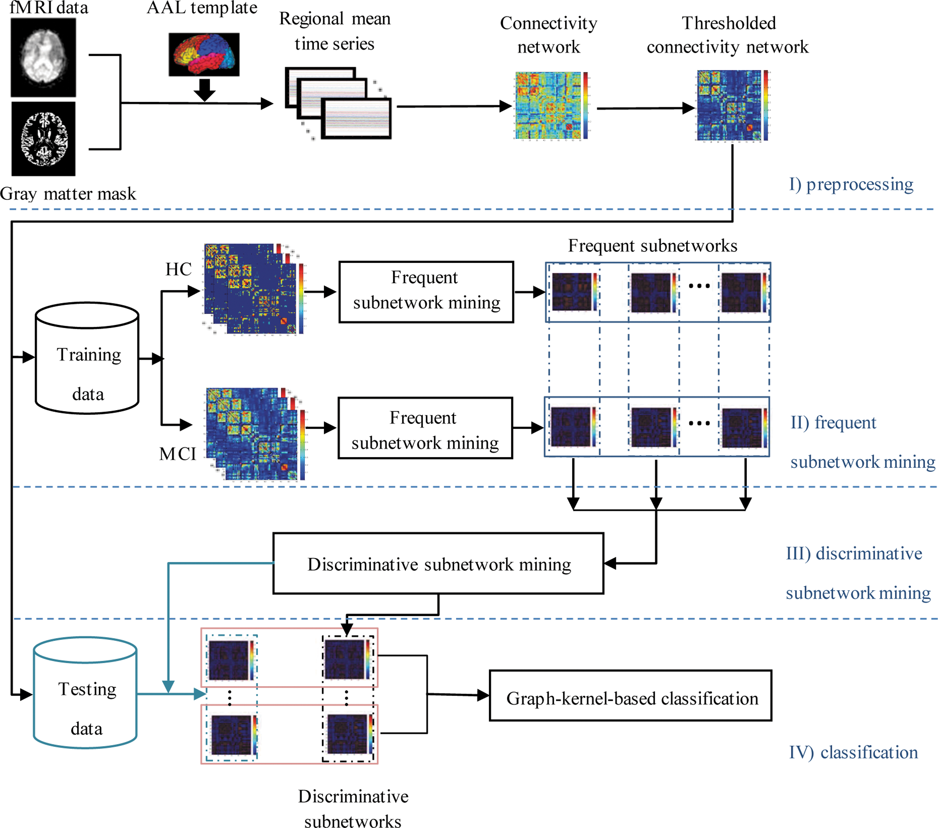
The framework of the proposed method. AAL, automated anatomical labeling; fMRI, functional magnetic resonance imaging; HC, healthy controls; MCI, mild cognitive impairment. Color images available online at www.liebertpub.com/brain

Preprocessing

The authors followed a similar procedure as in (Jie et al., 2013b). Specifically, the fMRI images were first preprocessed by applying the typical procedures of slice timing, motion correction, and spatial normalization using the Statistical Parametric Mapping software package (SPM8) (www.fil.ion.ucl.ac.uk.spm). Then, the brain space of fMRI images of each subject was parcellated into 116 regions-of-interest (ROIs) based on the automated anatomical labeling (AAL) atlas (Tzourio-Mazoyer et al., 2002). It is worth noting that in the current study, the authors used all the 116 ROIs from whole brain, including the cerebrum and cerebellar, instead of only 90 ROIs from the cerebrum as in (Jie et al., 2013b). The mean fMRI time series of each subject were then computed by averaging the GM-masked fMRI time series of the voxels in the ROI. In many studies, the GM-masked mean time series of each region was bandpass filtered within the frequency interval (0.01≤f≤0.1 Hz) (van den Heuvel and Pol, 2010). It is reported in (Zuo et al., 2010) that the frequency band of (0.027–0.073 Hz) demonstrated a significantly higher test–retest reliability than other frequency bands. It provides a reasonable trade-off between avoiding the physiological noise associated with higher frequency oscillations (Cordes et al., 2001) and the measurement error associated with estimating very low-frequency correlations from limited time series (Achard et al., 2008; Fornito et al., 2010). In this study, following the previous work (Jie et al., 2013b), the frequency band of (0.025–0.100 Hz) is used since the fMRI dynamics of neuronal activities are most salient within this frequency interval (Wee et al., 2012b). Thus, for each subject, a functional connectivity network was constructed with each ROI as a node, and the Pearson correlation between ROIs as connectivity strength. Fisher's r-to-z transformation (Davey et al., 2013) was applied on the elements of the functional connectivity network to improve the normality of the correlation coefficients as \documentclass{aastex}\usepackage{amsbsy}\usepackage{amsfonts}\usepackage{amssymb}\usepackage{bm}\usepackage{mathrsfs}\usepackage{pifont}\usepackage{stmaryrd}\usepackage{textcomp}\usepackage{portland, xspace}\usepackage{amsmath, amsxtra}\pagestyle{empty}\DeclareMathSizes{10}{9}{7}{6}\begin{document} \begin{align*} z = 0.5 [\ln (1 + r) - \ln (1 - r)] \tag{1} \end{align*} \end{document}

where r is the Pearson correlation coefficient and z is approximately a normal distribution with standard deviation \documentclass{aastex}\usepackage{amsbsy}\usepackage{amsfonts}\usepackage{amssymb}\usepackage{bm}\usepackage{mathrsfs}\usepackage{pifont}\usepackage{stmaryrd}\usepackage{textcomp}\usepackage{portland, xspace}\usepackage{amsmath, amsxtra}\pagestyle{empty}\DeclareMathSizes{10}{9}{7}{6}\begin{document}$$\sigma_z = 1 / \sqrt{n - 1}$$ \end{document} , where n is the number of ROIs. Moreover, to better analyze the topological property of network, the functional connectivity network was thresholded using a predefined value.

Frequent subnetwork (subgraph) mining

In this section, the authors introduce the frequent subgraph mining algorithm to discover the most frequent subnetwork patterns for MCI and HC, respectively. In the data mining community, a number of methods have been proposed for frequent subgraph mining (Borgelt and Berthold, 2002; Huan et al., 2003; Yan and Han, 2002). For example, FSG (Kuramochi and Karypis, 2004) finds all frequent subgraph connected subgraphs by using the breadth-first search strategy to grow candidates, whereby pairs of identified frequent k subgraphs are joined to generate (k+1) subgraphs. Apriori-based graph mining (Inokuchi et al., 2000) uses an adjacency matrix to represent graphs, and a levelwise search to discover frequent subgraphs. For more methods on frequent subgraph mining, please refer to (Jiang et al., 2013) for a recent review. In this study, the authors adopt the well-known gSpan algorithm (Yan and Han, 2002) for mining the frequent subnetworks (subgraphs) from the functional connectivity networks because of its time efficiency (Krishna et al., 2011). Before giving the details of gSpan, there are some preliminaries used to derive the gSpan algorithm (Yan and Han, 2002) for frequent subgraph mining.

Definition 1 (Labeled Undirected Graph)

Let G=(V, E, L, l) be a labeled undirected graph, where V is a set of nodes and E⊆V×V is a set of edges. e={u,v} indicates an edge between the nodes u and v. L is a set of labels, and l is a mapping function that assigns labels to vertices in V and edges in E.

Definition 2 (Subgraph)

For two labeled undirected graphs, G_s =(V_s , E_s , L_s , l_s ) and G=(V, E, L, l), G_s is a subgraph of G if V_s ⊆V, E_s ⊆E, L_s ⊆L, and l_s =l.

Definition 3 (Graph Isomorphism)

A graph \documentclass{aastex}\usepackage{amsbsy}\usepackage{amsfonts}\usepackage{amssymb}\usepackage{bm}\usepackage{mathrsfs}\usepackage{pifont}\usepackage{stmaryrd}\usepackage{textcomp}\usepackage{portland, xspace}\usepackage{amsmath, amsxtra}\pagestyle{empty}\DeclareMathSizes{10}{9}{7}{6}\begin{document}$$G_1 ( V_1 , E_1 , L_{V_{1}} , L_{E_{1}} , \varphi_1 )$$ \end{document} is isomorphic to another graph \documentclass{aastex}\usepackage{amsbsy}\usepackage{amsfonts}\usepackage{amssymb}\usepackage{bm}\usepackage{mathrsfs}\usepackage{pifont}\usepackage{stmaryrd}\usepackage{textcomp}\usepackage{portland, xspace}\usepackage{amsmath, amsxtra}\pagestyle{empty}\DeclareMathSizes{10}{9}{7}{6}\begin{document}$$G_2 ( V_2 , E_2 , L_{V_{2}} , L_{E_{2}} , \varphi_2 )$$ \end{document} , if and only a bijection f : V ₁→V ₂ exists such that (i) \documentclass{aastex}\usepackage{amsbsy}\usepackage{amsfonts}\usepackage{amssymb}\usepackage{bm}\usepackage{mathrsfs}\usepackage{pifont}\usepackage{stmaryrd}\usepackage{textcomp}\usepackage{portland, xspace}\usepackage{amsmath, amsxtra}\pagestyle{empty}\DeclareMathSizes{10}{9}{7}{6}\begin{document}$$\forall u \in V_1 , \varphi_1 ( u ) = \varphi_2 (\, f ( u ) )$$ \end{document} , (ii) \documentclass{aastex}\usepackage{amsbsy}\usepackage{amsfonts}\usepackage{amssymb}\usepackage{bm}\usepackage{mathrsfs}\usepackage{pifont}\usepackage{stmaryrd}\usepackage{textcomp}\usepackage{portland, xspace}\usepackage{amsmath, amsxtra}\pagestyle{empty}\DeclareMathSizes{10}{9}{7}{6}\begin{document}$$\forall ( u , v ) \in E_1 \leftrightarrow (\, f ( u ) , f ( v ) ) \in E_2$$ \end{document} , (iii) \documentclass{aastex}\usepackage{amsbsy}\usepackage{amsfonts}\usepackage{amssymb}\usepackage{bm}\usepackage{mathrsfs}\usepackage{pifont}\usepackage{stmaryrd}\usepackage{textcomp}\usepackage{portland, xspace}\usepackage{amsmath, amsxtra}\pagestyle{empty}\DeclareMathSizes{10}{9}{7}{6}\begin{document}$$\forall ( u , v ) \in E_1 ,\varphi_1 ( u , v ) =\varphi_2 (\, f ( u ) , f ( v ) )$$ \end{document} . The bijection f is an isomorphism between G ₁ and G ₂.

Definition 4 (Subgraph Frequency Ratio)

Given a set of graphs, \documentclass{aastex}\usepackage{amsbsy}\usepackage{amsfonts}\usepackage{amssymb}\usepackage{bm}\usepackage{mathrsfs}\usepackage{pifont}\usepackage{stmaryrd}\usepackage{textcomp}\usepackage{portland, xspace}\usepackage{amsmath, amsxtra}\pagestyle{empty}\DeclareMathSizes{10}{9}{7}{6}\begin{document}$${\mathbb G}$$ \end{document} , the frequency ratio of a subgraph g_s , is defined as \documentclass{aastex}\usepackage{amsbsy}\usepackage{amsfonts}\usepackage{amssymb}\usepackage{bm}\usepackage{mathrsfs}\usepackage{pifont}\usepackage{stmaryrd}\usepackage{textcomp}\usepackage{portland, xspace}\usepackage{amsmath, amsxtra}\pagestyle{empty}\DeclareMathSizes{10}{9}{7}{6}\begin{document} \begin{align*} fq \left( {\rm g} _s \mid {\mathbb G} \right) = \frac {\mid {\rm g} _s \ \hbox {is a subgraph of g and g} \in {\mathbb G} \mid} {\mid {\mathbb G} \mid} \end{align*} \end{document}

Definition 5 (Frequent Subgraph)

Given a set of graphs, \documentclass{aastex}\usepackage{amsbsy}\usepackage{amsfonts}\usepackage{amssymb}\usepackage{bm}\usepackage{mathrsfs}\usepackage{pifont}\usepackage{stmaryrd}\usepackage{textcomp}\usepackage{portland, xspace}\usepackage{amsmath, amsxtra}\pagestyle{empty}\DeclareMathSizes{10}{9}{7}{6}\begin{document}$${\mathbb G}$$ \end{document} and a support parameter s, a subgraph g_s is a frequent subgraph if and only g_s exists in at least \documentclass{aastex}\usepackage{amsbsy}\usepackage{amsfonts}\usepackage{amssymb}\usepackage{bm}\usepackage{mathrsfs}\usepackage{pifont}\usepackage{stmaryrd}\usepackage{textcomp}\usepackage{portland, xspace}\usepackage{amsmath, amsxtra}\pagestyle{empty}\DeclareMathSizes{10}{9}{7}{6}\begin{document}$$s \cdot \mid {\mathbb G} \mid$$ \end{document} of the input graph set.

Definition 6 (Frequent Subgraph Mining)

Given a set of labeled undirected graphs, \documentclass{aastex}\usepackage{amsbsy}\usepackage{amsfonts}\usepackage{amssymb}\usepackage{bm}\usepackage{mathrsfs}\usepackage{pifont}\usepackage{stmaryrd}\usepackage{textcomp}\usepackage{portland, xspace}\usepackage{amsmath, amsxtra}\pagestyle{empty}\DeclareMathSizes{10}{9}{7}{6}\begin{document}$${\mathbb G}$$ \end{document} and a support parameter s, where 0<s≤1, find all undirected graphs that are subgraphs in at least \documentclass{aastex}\usepackage{amsbsy}\usepackage{amsfonts}\usepackage{amssymb}\usepackage{bm}\usepackage{mathrsfs}\usepackage{pifont}\usepackage{stmaryrd}\usepackage{textcomp}\usepackage{portland, xspace}\usepackage{amsmath, amsxtra}\pagestyle{empty}\DeclareMathSizes{10}{9}{7}{6}\begin{document}$$s \cdot \mid {\mathbb G} \mid$$ \end{document} of the input graphs.

Definition 7 (Intersect-graph)

Given two graphs, G ₁=(V ₁, E ₁) and G ₂=(V ₂, E ₂), the intersect-graph G′=(V′, E′) (denoted as G ₁∩G ₂) is defined as E′=E ₁∩E ₂, all the nodes in edges set E′ form the nodes set V′.

Definition 8 (depth-first search [DFS] code)

Given a DFS tree T for a graph G, an edge sequence (e_i ) can be constructed based on \documentclass{aastex}\usepackage{amsbsy}\usepackage{amsfonts}\usepackage{amssymb}\usepackage{bm}\usepackage{mathrsfs}\usepackage{pifont}\usepackage{stmaryrd}\usepackage{textcomp}\usepackage{portland, xspace}\usepackage{amsmath, amsxtra}\pagestyle{empty}\DeclareMathSizes{10}{9}{7}{6}\begin{document}$$\prec_T$$ \end{document} , such that \documentclass{aastex}\usepackage{amsbsy}\usepackage{amsfonts}\usepackage{amssymb}\usepackage{bm}\usepackage{mathrsfs}\usepackage{pifont}\usepackage{stmaryrd}\usepackage{textcomp}\usepackage{portland, xspace}\usepackage{amsmath, amsxtra}\pagestyle{empty}\DeclareMathSizes{10}{9}{7}{6}\begin{document}$$e_i \prec_T e_{i + 1}$$ \end{document} , where \documentclass{aastex}\usepackage{amsbsy}\usepackage{amsfonts}\usepackage{amssymb}\usepackage{bm}\usepackage{mathrsfs}\usepackage{pifont}\usepackage{stmaryrd}\usepackage{textcomp}\usepackage{portland, xspace}\usepackage{amsmath, amsxtra}\pagestyle{empty}\DeclareMathSizes{10}{9}{7}{6}\begin{document}$$i = 0 , \ldots , \mid E \mid - 1$$ \end{document} . (e_i ) is called a DFS code, denoted as code (G,T).

DFS lexicographic order

In this subsection, the authors introduce how gSpan maps each graph into a unique minimum DFS code (Yan and Han, 2002). The authors use subscripts to label the nodes in terms of the DFS order. The node v_i is discovered befor node v_j if i<j. For the DFS tree, all the edges in the DFS tree are called forward-edge, and the edges that are not in the DFS tree are called backward-edge. A linear order, \documentclass{aastex}\usepackage{amsbsy}\usepackage{amsfonts}\usepackage{amssymb}\usepackage{bm}\usepackage{mathrsfs}\usepackage{pifont}\usepackage{stmaryrd}\usepackage{textcomp}\usepackage{portland, xspace}\usepackage{amsmath, amsxtra}\pagestyle{empty}\DeclareMathSizes{10}{9}{7}{6}\begin{document}$$\prec_T$$ \end{document} , is built among all the edges in graph G by the following rules (assume e ₁=(i ₁, j ₁), e ₂=(i ₂, j ₂)): (i) if i ₁=i ₂ and j ₁<j ₂, \documentclass{aastex}\usepackage{amsbsy}\usepackage{amsfonts}\usepackage{amssymb}\usepackage{bm}\usepackage{mathrsfs}\usepackage{pifont}\usepackage{stmaryrd}\usepackage{textcomp}\usepackage{portland, xspace}\usepackage{amsmath, amsxtra}\pagestyle{empty}\DeclareMathSizes{10}{9}{7}{6}\begin{document}$$e_1 \prec_T e_2$$ \end{document} ; (ii) if i ₁<i ₂ and j ₁=j ₂, \documentclass{aastex}\usepackage{amsbsy}\usepackage{amsfonts}\usepackage{amssymb}\usepackage{bm}\usepackage{mathrsfs}\usepackage{pifont}\usepackage{stmaryrd}\usepackage{textcomp}\usepackage{portland, xspace}\usepackage{amsmath, amsxtra}\pagestyle{empty}\DeclareMathSizes{10}{9}{7}{6}\begin{document}$$e_1 \prec_T e_2$$ \end{document} ; and (iii) if \documentclass{aastex}\usepackage{amsbsy}\usepackage{amsfonts}\usepackage{amssymb}\usepackage{bm}\usepackage{mathrsfs}\usepackage{pifont}\usepackage{stmaryrd}\usepackage{textcomp}\usepackage{portland, xspace}\usepackage{amsmath, amsxtra}\pagestyle{empty}\DeclareMathSizes{10}{9}{7}{6}\begin{document}$$e_1 \prec_T e_2$$ \end{document} and \documentclass{aastex}\usepackage{amsbsy}\usepackage{amsfonts}\usepackage{amssymb}\usepackage{bm}\usepackage{mathrsfs}\usepackage{pifont}\usepackage{stmaryrd}\usepackage{textcomp}\usepackage{portland, xspace}\usepackage{amsmath, amsxtra}\pagestyle{empty}\DeclareMathSizes{10}{9}{7}{6}\begin{document}$$e_2 \prec_T e_3$$ \end{document} , \documentclass{aastex}\usepackage{amsbsy}\usepackage{amsfonts}\usepackage{amssymb}\usepackage{bm}\usepackage{mathrsfs}\usepackage{pifont}\usepackage{stmaryrd}\usepackage{textcomp}\usepackage{portland, xspace}\usepackage{amsmath, amsxtra}\pagestyle{empty}\DeclareMathSizes{10}{9}{7}{6}\begin{document}$$e_1 \prec_T e_3$$ \end{document} .

Then, an edge can be simply represented by a five-tuple (i, j,l ₁, l _(i,j), l _j). In this study, l_i and l_j are the labels of v_i and v_j , respectively, and l_(i,j) is the label of the edge (v_i, v_j ).

The DFS lexicographic order is a linear order defined as follows: \documentclass{aastex}\usepackage{amsbsy}\usepackage{amsfonts}\usepackage{amssymb}\usepackage{bm}\usepackage{mathrsfs}\usepackage{pifont}\usepackage{stmaryrd}\usepackage{textcomp}\usepackage{portland, xspace}\usepackage{amsmath, amsxtra}\pagestyle{empty}\DeclareMathSizes{10}{9}{7}{6}\begin{document}$$\alpha = ( \alpha_0 , \alpha_1 , \ldots , \alpha_m )$$ \end{document} and \documentclass{aastex}\usepackage{amsbsy}\usepackage{amsfonts}\usepackage{amssymb}\usepackage{bm}\usepackage{mathrsfs}\usepackage{pifont}\usepackage{stmaryrd}\usepackage{textcomp}\usepackage{portland, xspace}\usepackage{amsmath, amsxtra}\pagestyle{empty}\DeclareMathSizes{10}{9}{7}{6}\begin{document}$$\beta = ( \beta_0 , \beta_1 , \ldots , \beta_m )$$ \end{document} are DFS codes, then α≤β if either of the following is true (Yan and Han, 2002):

(i) \documentclass{aastex}\usepackage{amsbsy}\usepackage{amsfonts}\usepackage{amssymb}\usepackage{bm}\usepackage{mathrsfs}\usepackage{pifont}\usepackage{stmaryrd}\usepackage{textcomp}\usepackage{portland, xspace}\usepackage{amsmath, amsxtra}\pagestyle{empty}\DeclareMathSizes{10}{9}{7}{6}\begin{document}$$\exists t , 0 \leq t \leq \min ( m , n ) , \alpha_k = \beta_k \ for \ k < t , \alpha_t \prec_e \beta_t$$ \end{document}

(ii) \documentclass{aastex}\usepackage{amsbsy}\usepackage{amsfonts}\usepackage{amssymb}\usepackage{bm}\usepackage{mathrsfs}\usepackage{pifont}\usepackage{stmaryrd}\usepackage{textcomp}\usepackage{portland, xspace}\usepackage{amsmath, amsxtra}\pagestyle{empty}\DeclareMathSizes{10}{9}{7}{6}\begin{document}$$\alpha_k = \beta_k \ for \ 0 \leq k \leq m , \ and \ n \geq m$$ \end{document}

Given a graph G, the minimum one of all the DFS lexicographic order is called Minimum DFS Code of G. It is also a canonical label of G. Figure 2 shows a DFS code tree, where all the minimum DFS codes of frequent subgraphs can be discovered through DFS of the code tree. It is noteworthy that the red nodes contain the same subgraph with different DFS codes, but g′ is not the minimum DFS code, so the whole branch of g′ can be pruned because it will not contain any minimum DFS code.

FIG. 2.

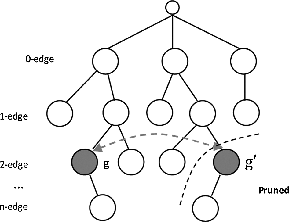
A search space: DFS code tree. DFS, depth-first search.

In summary, gSpan first constructs a new lexicographic order among graphs, and maps each graph into a unique minimum DFS code as its canonical label. Then, based on the lexicographic order, gSpan utilizes the DFS strategy to mine frequent connected subgraph patterns efficiently. In this study, the hierarchical search space of frequent subgraph is called a DFS code tree, and each node of the search tree represents a DFS code (i.e., subgraph). The k+1-th level subgraph is generated from the k-th level subgraph (i.e., parent) by adding one frequent edge. Finally, all subgraphs with nonminimal DFS code are pruned to avoid redundant candidate generations (Yan and Han, 2002).

In the Appendix 1, there is a toy example to illustrate the DFS lexicographic order used in frequent subgraph mining and also list the detailed gSpan algorithm (see algorithm 3).

Discriminative subnetwork mining

In the previous section, the authors have introduced the gSpan algorithm. It is worth noting that gSpan is only used for mining the frequent subgraph, which by itself does not have any discriminative power. Accordingly, in this study, the authors perform gSpan to extract two sets of frequent subgraphs (e.g., subnetworks) from the MCI group and HC group, respectively. However, some of the frequent subnetworks may still have less discriminative information for classification. To address that problem, it is further proposed to select the most discriminative subnetworks from those frequent subnetworks using a graph kernel-based classification method. In the following, the authors first introduce the graph kernel technique.

Graph kernel

Roughly speaking, kernel can be seen as a similarity measure between a pair of subjects, which maps the data from the original space into a higher dimensional feature space, where the data are more likely to be linear separable. Given two subjects x sand x′, the kernel can be defined as \documentclass{aastex}\usepackage{amsbsy}\usepackage{amsfonts}\usepackage{amssymb}\usepackage{bm}\usepackage{mathrsfs}\usepackage{pifont}\usepackage{stmaryrd}\usepackage{textcomp}\usepackage{portland, xspace}\usepackage{amsmath, amsxtra}\pagestyle{empty}\DeclareMathSizes{10}{9}{7}{6}\begin{document} \begin{align*} k (x , x{\prime}) = < \phi (x) , \phi (x {\prime}) > \tag{2} \end{align*} \end{document}

where φ is a mapping function that maps data from input space to feature space. Besides the feature vector, kernel can also be applied on more complex data types, for example, graph, with the corresponding kernel called graph kernel (Vishwanathan et al., 2010). Graph kernel can be seen as a function that measures the topological similarity of pairs of graphs. In recent years, lots of methods have been proposed to construct graph kernel, which include walk-based (Gartner et al., 2003), path-based (Alvarez et al., 2011), subtree-based kernels (Shervashidze et al., 2011), and so on. Graph kernel has been widely used for image classification (Harchaoui and Bach, 2007) and protein function prediction (Borgwardt et al., 2005).

In this study, following the previous work (Jie et al., 2013b), the authors adopt the Weisfeiler-Lehman subtree kernel, which is based on the Weisfeiler-Lehman test of isomorphism (Shervashidze et al., 2011). Given two graphs, the basic process of the Weisfeiler-Lehman test is as follows: if those two graphs are unlabeled (i.e., vertices of the graph have not been assigned labels), first label each vertex with the number of edges that are connected to that vertex. Then, at each iteration step, the label of each vertex is updated based on its previous label and the labels of its neighbors. That is, compress the sorted set of updated node labels of each vertex into a new and shorter label. This process iterates until the node label sets are identical, or the number of iteration reaches its predefined maximum value.

Given two graphs G and H, let \documentclass{aastex}\usepackage{amsbsy}\usepackage{amsfonts}\usepackage{amssymb}\usepackage{bm}\usepackage{mathrsfs}\usepackage{pifont}\usepackage{stmaryrd}\usepackage{textcomp}\usepackage{portland, xspace}\usepackage{amsmath, amsxtra}\pagestyle{empty}\DeclareMathSizes{10}{9}{7}{6}\begin{document}$$\scriptstyle\sum_0$$ \end{document} be the original set of node labels of G and H, and \documentclass{aastex}\usepackage{amsbsy}\usepackage{amsfonts}\usepackage{amssymb}\usepackage{bm}\usepackage{mathrsfs}\usepackage{pifont}\usepackage{stmaryrd}\usepackage{textcomp}\usepackage{portland, xspace}\usepackage{amsmath, amsxtra}\pagestyle{empty}\DeclareMathSizes{10}{9}{7}{6}\begin{document}$$\scriptstyle\sum_i$$ \end{document} be the set of letters that occur as node labels at least once in G or H at the end of the i-th iteration of the Weisfeiler-Lehman algorithm. Assume that all \documentclass{aastex}\usepackage{amsbsy}\usepackage{amsfonts}\usepackage{amssymb}\usepackage{bm}\usepackage{mathrsfs}\usepackage{pifont}\usepackage{stmaryrd}\usepackage{textcomp}\usepackage{portland, xspace}\usepackage{amsmath, amsxtra}\pagestyle{empty}\DeclareMathSizes{10}{9}{7}{6}\begin{document}$${\sum}_i = \big\{ \sigma_{i1} , \sigma_{i2} , \ldots , \sigma_{i \mid \sum_i \mid } \big\} $$ \end{document} are pairwise disjointed. Without loss of generality, assume every \documentclass{aastex}\usepackage{amsbsy}\usepackage{amsfonts}\usepackage{amssymb}\usepackage{bm}\usepackage{mathrsfs}\usepackage{pifont}\usepackage{stmaryrd}\usepackage{textcomp}\usepackage{portland, xspace}\usepackage{amsmath, amsxtra}\pagestyle{empty}\DeclareMathSizes{10}{9}{7}{6}\begin{document}$$\sum_i$$ \end{document} is ordered. The Weisfeiler-Lehman subtree kernel on two graphs G and H with h iterations is defined as follows (Shervashidze et al., 2011): \documentclass{aastex}\usepackage{amsbsy}\usepackage{amsfonts}\usepackage{amssymb}\usepackage{bm}\usepackage{mathrsfs}\usepackage{pifont}\usepackage{stmaryrd}\usepackage{textcomp}\usepackage{portland, xspace}\usepackage{amsmath, amsxtra}\pagestyle{empty}\DeclareMathSizes{10}{9}{7}{6}\begin{document} \begin{align*} k^h (G , H) \,= < \phi^h (G) , \phi^h (H) > \tag{3} \end{align*} \end{document}

where \documentclass{aastex}\usepackage{amsbsy}\usepackage{amsfonts}\usepackage{amssymb}\usepackage{bm}\usepackage{mathrsfs}\usepackage{pifont}\usepackage{stmaryrd}\usepackage{textcomp}\usepackage{portland, xspace}\usepackage{amsmath, amsxtra}\pagestyle{empty}\DeclareMathSizes{10}{9}{7}{6}\begin{document} \begin{align*} \phi^h (G) = \Big( c_0 (G , \sigma_{01}) , \ldots , c_0 \Big( G , \sigma_{0 \mid \sum_0 \mid} \Big) , \ldots , \\ \quad c_h ( G , \sigma_{h1} ) , \ldots , c_h \Big( G , \sigma_{h \mid \sum_h \mid } \Big)\Big) \end{align*} \end{document}

and \documentclass{aastex}\usepackage{amsbsy}\usepackage{amsfonts}\usepackage{amssymb}\usepackage{bm}\usepackage{mathrsfs}\usepackage{pifont}\usepackage{stmaryrd}\usepackage{textcomp}\usepackage{portland, xspace}\usepackage{amsmath, amsxtra}\pagestyle{empty}\DeclareMathSizes{10}{9}{7}{6}\begin{document} \begin{align*} \phi^h ( H ) = \Big( c_0 ( H , \sigma_{01} ) , \ldots, c_0 \Big( H , \sigma_{0 \mid \sum_0 \mid } \Big) , \ldots , \\\quad c_h ( H , \sigma_{h1} ) , \ldots , c_h \Big( H , \sigma_{h \mid \sum_h \mid } \Big)\Big). \end{align*} \end{document}

In this study, c_i (G, σ_ij) and c_i (H, σ_ij) are the number of occurrences of the node label σ_ij in G and H with the i-th iteration, respectively. It is noteworthy that the graph used in this study is the undirected graph.

The DSM algorithm

The authors first choose the same number of frequent subnetworks from each group and construct multiple pairs of subnetworks across two groups. It is noteworthy that each pair of frequent subnetworks represents two types of connectivity patterns from patient and normal controls. For each pair of frequent subnetworks, they utilized graph kernel proposed in (Shervashidze et al., 2011) to measure the similarity between the training data and the frequent subnetworks and classify the training data to the class with a high graph kernel value. Figure 3 gives a toy example of how to measure the similarity between brain networks. After that, the authors choose those pairs of frequent subnetworks with the best classification accuracy as the most discriminative subnetworks.

FIG. 3.

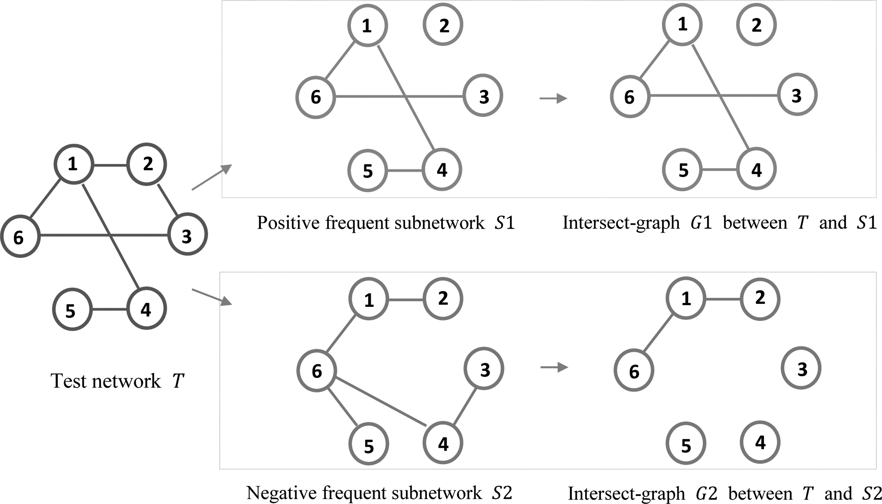
Illustration on similarity comparison between brain networks. In this study, the similarity between G1 and S1 is 12, while the similarity between G2 and S2 is 8. The similarity is measured by Weisfeiler-Lehman subtree kernel after 1st iteration.

Algorithm 1 summarizes the details of the proposed DSM algorithm. In this study, \documentclass{aastex}\usepackage{amsbsy}\usepackage{amsfonts}\usepackage{amssymb}\usepackage{bm}\usepackage{mathrsfs}\usepackage{pifont}\usepackage{stmaryrd}\usepackage{textcomp}\usepackage{portland, xspace}\usepackage{amsmath, amsxtra}\pagestyle{empty}\DeclareMathSizes{10}{9}{7}{6}\begin{document}$${\mathbb D}$$ \end{document} denotes the training set, including the functional connectivity networks of all training subjects, and \documentclass{aastex}\usepackage{amsbsy}\usepackage{amsfonts}\usepackage{amssymb}\usepackage{bm}\usepackage{mathrsfs}\usepackage{pifont}\usepackage{stmaryrd}\usepackage{textcomp}\usepackage{portland, xspace}\usepackage{amsmath, amsxtra}\pagestyle{empty}\DeclareMathSizes{10}{9}{7}{6}\begin{document}$${\mathbb MCI}$$ \end{document} and \documentclass{aastex}\usepackage{amsbsy}\usepackage{amsfonts}\usepackage{amssymb}\usepackage{bm}\usepackage{mathrsfs}\usepackage{pifont}\usepackage{stmaryrd}\usepackage{textcomp}\usepackage{portland, xspace}\usepackage{amsmath, amsxtra}\pagestyle{empty}\DeclareMathSizes{10}{9}{7}{6}\begin{document}$${\mathbb HC}$$ \end{document} represent the MCI and HC groups on the training set, respectively. Let G_i denote a sample in the dataset and y_i be the corresponding label, and S ₁ and S ₂ are two sets of frequent subnetworks mined from the MCI and HC groups, respectively. Also, \documentclass{aastex}\usepackage{amsbsy}\usepackage{amsfonts}\usepackage{amssymb}\usepackage{bm}\usepackage{mathrsfs}\usepackage{pifont}\usepackage{stmaryrd}\usepackage{textcomp}\usepackage{portland, xspace}\usepackage{amsmath, amsxtra}\pagestyle{empty}\DeclareMathSizes{10}{9}{7}{6}\begin{document}$$S_1^i ( S_2^i )$$ \end{document} represents the i-th subnetwork in S ₁ (S ₂), and \documentclass{aastex}\usepackage{amsbsy}\usepackage{amsfonts}\usepackage{amssymb}\usepackage{bm}\usepackage{mathrsfs}\usepackage{pifont}\usepackage{stmaryrd}\usepackage{textcomp}\usepackage{portland, xspace}\usepackage{amsmath, amsxtra}\pagestyle{empty}\DeclareMathSizes{10}{9}{7}{6}\begin{document}$$G_1^i ( G_2^i )$$ \end{document} is the i-th intersect graph between G and \documentclass{aastex}\usepackage{amsbsy}\usepackage{amsfonts}\usepackage{amssymb}\usepackage{bm}\usepackage{mathrsfs}\usepackage{pifont}\usepackage{stmaryrd}\usepackage{textcomp}\usepackage{portland, xspace}\usepackage{amsmath, amsxtra}\pagestyle{empty}\DeclareMathSizes{10}{9}{7}{6}\begin{document}$$S_1^i ( S_2^i )$$ \end{document} . Finally, DS ₁ and DS ₂ are two sets of selected discriminative subnetworks of MCI and HC, respectively.

Algorithm 1 Discriminative Subnetwork Mining (DSM) Input:

Training subjects \documentclass{aastex}\usepackage{amsbsy}\usepackage{amsfonts}\usepackage{amssymb}\usepackage{bm}\usepackage{mathrsfs}\usepackage{pifont}\usepackage{stmaryrd}\usepackage{textcomp}\usepackage{portland, xspace}\usepackage{amsmath, amsxtra}\pagestyle{empty}\DeclareMathSizes{10}{9}{7}{6}\begin{document}$${\mathbb D} = \{ {\mathbb MCI} , \ {\mathbb HC} \} = \{ ( G_1 , y_1 ) , \ldots , ( G_i , y_i ) , \ldots , ( G_N , y_N ) \}$$\end{document}

Output:

Two sets of discriminative subnetworks DS ₁ and DS ₂

1: \documentclass{aastex}\usepackage{amsbsy}\usepackage{amsfonts}\usepackage{amssymb}\usepackage{bm}\usepackage{mathrsfs}\usepackage{pifont}\usepackage{stmaryrd}\usepackage{textcomp}\usepackage{portland, xspace}\usepackage{amsmath, amsxtra}\pagestyle{empty}\DeclareMathSizes{10}{9}{7}{6}\begin{document}$${ \rm gSpan} ( {\mathbb MCI} , S_1 )$$\end{document} , \documentclass{aastex}\usepackage{amsbsy}\usepackage{amsfonts}\usepackage{amssymb}\usepackage{bm}\usepackage{mathrsfs}\usepackage{pifont}\usepackage{stmaryrd}\usepackage{textcomp}\usepackage{portland, xspace}\usepackage{amsmath, amsxtra}\pagestyle{empty}\DeclareMathSizes{10}{9}{7}{6}\begin{document}$${ \rm gSpan} ( {\mathbb HC} , S_2 )$$\end{document} ;

2: Initialize a temporary list C=[];

3: for i=1 : n do

4: for each \documentclass{aastex}\usepackage{amsbsy}\usepackage{amsfonts}\usepackage{amssymb}\usepackage{bm}\usepackage{mathrsfs}\usepackage{pifont}\usepackage{stmaryrd}\usepackage{textcomp}\usepackage{portland, xspace}\usepackage{amsmath, amsxtra}\pagestyle{empty}\DeclareMathSizes{10}{9}{7}{6}\begin{document}$$G \in {\mathbb D}$$\end{document} do

5: \documentclass{aastex}\usepackage{amsbsy}\usepackage{amsfonts}\usepackage{amssymb}\usepackage{bm}\usepackage{mathrsfs}\usepackage{pifont}\usepackage{stmaryrd}\usepackage{textcomp}\usepackage{portland, xspace}\usepackage{amsmath, amsxtra}\pagestyle{empty}\DeclareMathSizes{10}{9}{7}{6}\begin{document}$$G_1^i = G \cap S_1^i$$\end{document} , \documentclass{aastex}\usepackage{amsbsy}\usepackage{amsfonts}\usepackage{amssymb}\usepackage{bm}\usepackage{mathrsfs}\usepackage{pifont}\usepackage{stmaryrd}\usepackage{textcomp}\usepackage{portland, xspace}\usepackage{amsmath, amsxtra}\pagestyle{empty}\DeclareMathSizes{10}{9}{7}{6}\begin{document}$$G_2^i = G \cap S_2^i$$\end{document} ;

6: Compute the graph kernel using Eq. (3) on \documentclass{aastex}\usepackage{amsbsy}\usepackage{amsfonts}\usepackage{amssymb}\usepackage{bm}\usepackage{mathrsfs}\usepackage{pifont}\usepackage{stmaryrd}\usepackage{textcomp}\usepackage{portland, xspace}\usepackage{amsmath, amsxtra}\pagestyle{empty}\DeclareMathSizes{10}{9}{7}{6}\begin{document}$$G_1^i$$\end{document} , \documentclass{aastex}\usepackage{amsbsy}\usepackage{amsfonts}\usepackage{amssymb}\usepackage{bm}\usepackage{mathrsfs}\usepackage{pifont}\usepackage{stmaryrd}\usepackage{textcomp}\usepackage{portland, xspace}\usepackage{amsmath, amsxtra}\pagestyle{empty}\DeclareMathSizes{10}{9}{7}{6}\begin{document}$$S_1^i$$\end{document} and \documentclass{aastex}\usepackage{amsbsy}\usepackage{amsfonts}\usepackage{amssymb}\usepackage{bm}\usepackage{mathrsfs}\usepackage{pifont}\usepackage{stmaryrd}\usepackage{textcomp}\usepackage{portland, xspace}\usepackage{amsmath, amsxtra}\pagestyle{empty}\DeclareMathSizes{10}{9}{7}{6}\begin{document}$$G_2^i$$\end{document} , \documentclass{aastex}\usepackage{amsbsy}\usepackage{amsfonts}\usepackage{amssymb}\usepackage{bm}\usepackage{mathrsfs}\usepackage{pifont}\usepackage{stmaryrd}\usepackage{textcomp}\usepackage{portland, xspace}\usepackage{amsmath, amsxtra}\pagestyle{empty}\DeclareMathSizes{10}{9}{7}{6}\begin{document}$$S_2^i$$\end{document} , respectively;

7: Classify G to the class with larger graph kernel value;

8: endfor

9: Compute the accuracy c on \documentclass{aastex}\usepackage{amsbsy}\usepackage{amsfonts}\usepackage{amssymb}\usepackage{bm}\usepackage{mathrsfs}\usepackage{pifont}\usepackage{stmaryrd}\usepackage{textcomp}\usepackage{portland, xspace}\usepackage{amsmath, amsxtra}\pagestyle{empty}\DeclareMathSizes{10}{9}{7}{6}\begin{document}$${\mathbb D}$$\end{document} ;

10: Update list C=[C, c];

11: endfor

12: Sort S ₁, S ₂ according to the C in a descending order;

13: Select the top k subnetworks of S ₁ and S ₂ as discriminative subnetworks;

Classification

For classification of testing subject, the authors also compute the graph kernel between each discriminative subnetwork and the intersect graph between the testing subject and that discriminative subnetwork, and then perform a graph kernel-based classification. Specifically, the authors obtain two sets of graph kernel values, one by measuring the topological similarity (through graph kernel) between the subnetworks from the MCI group and corresponding intersect graph of the testing subject, and the other by measuring the similarity between the subnetworks from the HC group and corresponding intersect graph of the testing subject. Then, the authors classify the testing subject to the class with the highest graph kernel value. Algorithm 2 gives the detailed procedure of the graph kernel-based classification. In this study, DS ₁ and DS ₂ represent two sets of discriminative subnetworks, which are obtained using the DSM algorithm, G represents a graph in test subject set \documentclass{aastex}\usepackage{amsbsy}\usepackage{amsfonts}\usepackage{amssymb}\usepackage{bm}\usepackage{mathrsfs}\usepackage{pifont}\usepackage{stmaryrd}\usepackage{textcomp}\usepackage{portland, xspace}\usepackage{amsmath, amsxtra}\pagestyle{empty}\DeclareMathSizes{10}{9}{7}{6}\begin{document}$${\mathbb T}$$ \end{document} , and \documentclass{aastex}\usepackage{amsbsy}\usepackage{amsfonts}\usepackage{amssymb}\usepackage{bm}\usepackage{mathrsfs}\usepackage{pifont}\usepackage{stmaryrd}\usepackage{textcomp}\usepackage{portland, xspace}\usepackage{amsmath, amsxtra}\pagestyle{empty}\DeclareMathSizes{10}{9}{7}{6}\begin{document}$$G_1^i ( G_2^i )$$ \end{document} is the i-th intersect graph between G and \documentclass{aastex}\usepackage{amsbsy}\usepackage{amsfonts}\usepackage{amssymb}\usepackage{bm}\usepackage{mathrsfs}\usepackage{pifont}\usepackage{stmaryrd}\usepackage{textcomp}\usepackage{portland, xspace}\usepackage{amsmath, amsxtra}\pagestyle{empty}\DeclareMathSizes{10}{9}{7}{6}\begin{document}$$S_1^i ( S_2^i )$$ \end{document} .

Algorithm 2 Graph kernel-based Classification Input:

Discriminative subnetwork sets DS ₁ and DS ₂, testing subject set \documentclass{aastex}\usepackage{amsbsy}\usepackage{amsfonts}\usepackage{amssymb}\usepackage{bm}\usepackage{mathrsfs}\usepackage{pifont}\usepackage{stmaryrd}\usepackage{textcomp}\usepackage{portland, xspace}\usepackage{amsmath, amsxtra}\pagestyle{empty}\DeclareMathSizes{10}{9}{7}{6}\begin{document}$${\mathbb T}$$\end{document}

Output:

Classification accuracy acc

1: for each \documentclass{aastex}\usepackage{amsbsy}\usepackage{amsfonts}\usepackage{amssymb}\usepackage{bm}\usepackage{mathrsfs}\usepackage{pifont}\usepackage{stmaryrd}\usepackage{textcomp}\usepackage{portland, xspace}\usepackage{amsmath, amsxtra}\pagestyle{empty}\DeclareMathSizes{10}{9}{7}{6}\begin{document}$$G \in {\mathbb T}$$\end{document} do

2: for i=1 : k do

3: \documentclass{aastex}\usepackage{amsbsy}\usepackage{amsfonts}\usepackage{amssymb}\usepackage{bm}\usepackage{mathrsfs}\usepackage{pifont}\usepackage{stmaryrd}\usepackage{textcomp}\usepackage{portland, xspace}\usepackage{amsmath, amsxtra}\pagestyle{empty}\DeclareMathSizes{10}{9}{7}{6}\begin{document}$$G_1^i = G \cap DS_1^i$$\end{document} , \documentclass{aastex}\usepackage{amsbsy}\usepackage{amsfonts}\usepackage{amssymb}\usepackage{bm}\usepackage{mathrsfs}\usepackage{pifont}\usepackage{stmaryrd}\usepackage{textcomp}\usepackage{portland, xspace}\usepackage{amsmath, amsxtra}\pagestyle{empty}\DeclareMathSizes{10}{9}{7}{6}\begin{document}$$G_2^i = G \cap DS_2^i$$\end{document} ;

4: Compute the graph kernel on \documentclass{aastex}\usepackage{amsbsy}\usepackage{amsfonts}\usepackage{amssymb}\usepackage{bm}\usepackage{mathrsfs}\usepackage{pifont}\usepackage{stmaryrd}\usepackage{textcomp}\usepackage{portland, xspace}\usepackage{amsmath, amsxtra}\pagestyle{empty}\DeclareMathSizes{10}{9}{7}{6}\begin{document}$$G_1^i$$\end{document} , \documentclass{aastex}\usepackage{amsbsy}\usepackage{amsfonts}\usepackage{amssymb}\usepackage{bm}\usepackage{mathrsfs}\usepackage{pifont}\usepackage{stmaryrd}\usepackage{textcomp}\usepackage{portland, xspace}\usepackage{amsmath, amsxtra}\pagestyle{empty}\DeclareMathSizes{10}{9}{7}{6}\begin{document}$$DS_1^i$$\end{document} and \documentclass{aastex}\usepackage{amsbsy}\usepackage{amsfonts}\usepackage{amssymb}\usepackage{bm}\usepackage{mathrsfs}\usepackage{pifont}\usepackage{stmaryrd}\usepackage{textcomp}\usepackage{portland, xspace}\usepackage{amsmath, amsxtra}\pagestyle{empty}\DeclareMathSizes{10}{9}{7}{6}\begin{document}$$G_2^i$$\end{document} , \documentclass{aastex}\usepackage{amsbsy}\usepackage{amsfonts}\usepackage{amssymb}\usepackage{bm}\usepackage{mathrsfs}\usepackage{pifont}\usepackage{stmaryrd}\usepackage{textcomp}\usepackage{portland, xspace}\usepackage{amsmath, amsxtra}\pagestyle{empty}\DeclareMathSizes{10}{9}{7}{6}\begin{document}$$DS_2^i$$\end{document} , respectively;

5: endfor

6: Classify G to the class which has larger graph kernel value;

7: endfor

8: Compute the accuracy acc on \documentclass{aastex}\usepackage{amsbsy}\usepackage{amsfonts}\usepackage{amssymb}\usepackage{bm}\usepackage{mathrsfs}\usepackage{pifont}\usepackage{stmaryrd}\usepackage{textcomp}\usepackage{portland, xspace}\usepackage{amsmath, amsxtra}\pagestyle{empty}\DeclareMathSizes{10}{9}{7}{6}\begin{document}$${\mathbb T}$$\end{document}

Validation

To evaluate the performance of this method, the leave-one-out cross-validation strategy was adopted in the experiment. Specifically, at each fold, one subject was left out for testing and the remaining subjects were used for training, and this process was repeated for each subject. The authors use the classification accuracy and the area under the ROC curve (AUC) as performance measures to quantify the results. Specifically, classification accuracy measures the effectiveness of predicting the true class label. The AUC measures the probability that when one positive and one negative sample are drawn at random, the decision function assigns a higher value to the positive than to the negative sample.

The functional connectivity networks were thresholded by using a predefined threshold T=0.3 to validate the classification performance of the proposed method. The authors used the gSpan algorithm to search for frequent subnetworks in thresholded functional connectivity networks of MCI and HC with corresponding supports s=9/11 and s=22/24, respectively. The number of iteration h in Weisfeiler-Lehman subtree kernel algorithm was set as 3.

Results

Comparison on classification performance

In this section, the authors evaluate the classification performance of the proposed method by measuring the classification accuracy. For comparison, they also give the results of other functional connectivity networks-based classification methods, including (Jie et al., 2013b, 2014; Wee et al., 2012a). Specifically, the core of (Jie et al., 2013b) is using a graph kernel-based approach to measure the topological similarity between functional connectivity networks, and the method in (Jie et al., 2014) integrates multiple properties of connectivity (i.e., local clustering coefficients, and global topological properties) for improving the classification performance. Also, in (Wee et al., 2012a), the authors utilize a multispectrum strategy to construct multiple functional connectivity networks for each subject, and then local clustering coefficients are extracted as features for MCI classification. Table 2 gives the classification performances of all compared methods. As can be seen from Table 2, the proposed method achieves a best classification accuracy of 97.30% with an increment of at least 5.4% from all other compared methods. Actually, only one MCI subject is misclassified by this method. Also, this method outperforms all other methods in the AUC performance measure.

Table 2.

The Classification Performances of Different Methods

Methods	Accuracy (%)	AUC
Wee et al. (2012a)	86.49	0.8633
Jie et al. (2014)	91.89	0.8700
Jie et al. (2013b)	91.89	0.9400
Proposed	97.30	0.9583

The bold values are the best for comparison.

AUC, area under ROC curve.

The connectivity analysis

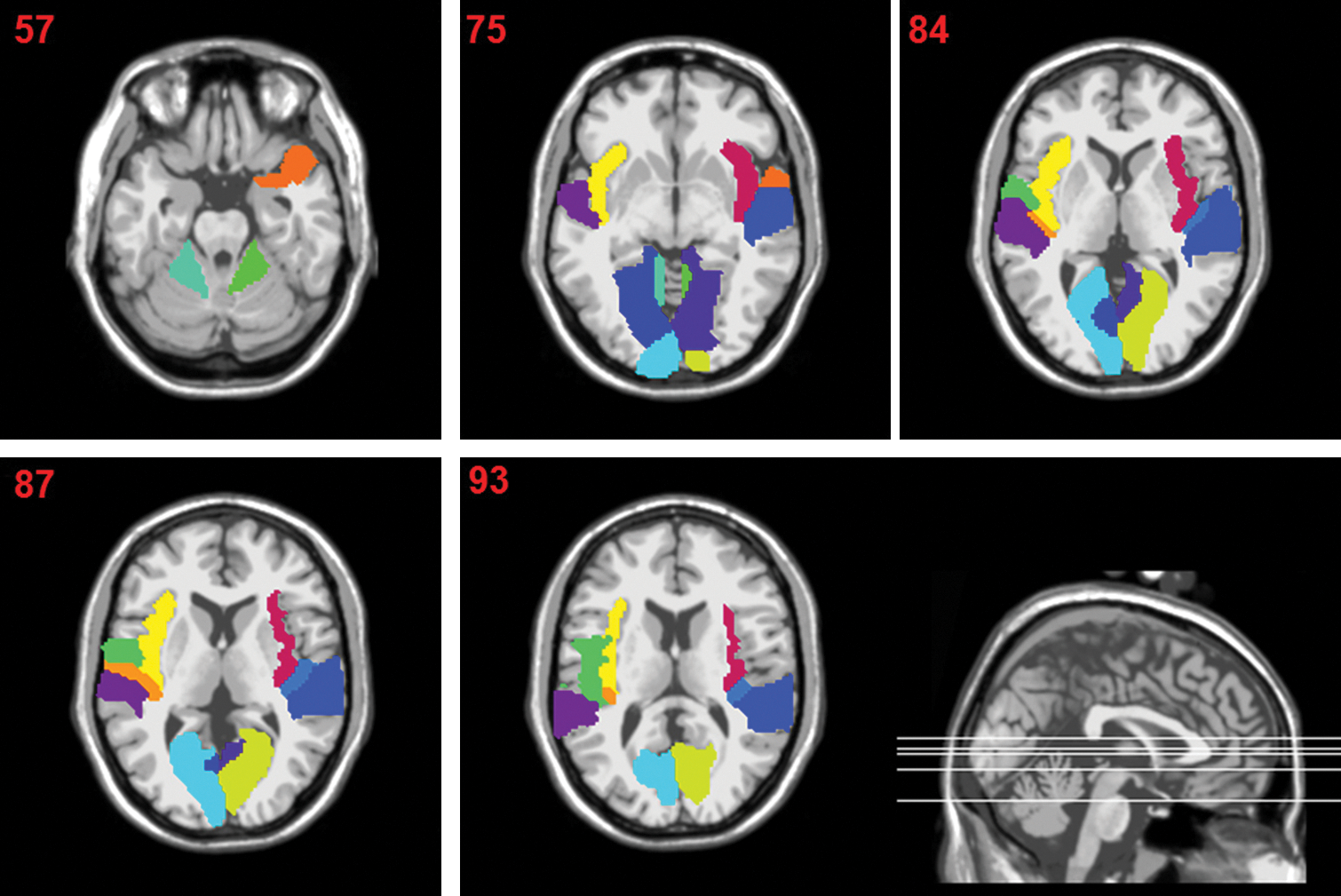
By mining the frequent and discriminative subnetworks of the functional connectivity networks for MCI and HC, this method may also help gain a better insight of the topological differences of the brain network between MCI and HC. Figure 4 shows the mined discriminative and frequent subnetworks from the MCI and HC groups. As can be seen from Figure 4, MCI and HC have very different connectivity patterns in the mined subnetworks. Specifically, compared with that of HC, there exist possible disruptions in the connectivity of MCI between certain regions that are consistent with existing findings reported in previous studies (Davatzikos et al., 2011; Grady et al., 2003; Han et al., 2011). For example, in HC, the mined frequent and discriminative subnetworks contain visual and auditory brain regions, with strong connections between these brain regions, while the connections in those brain regions are disrupted for MCI.

FIG. 4.

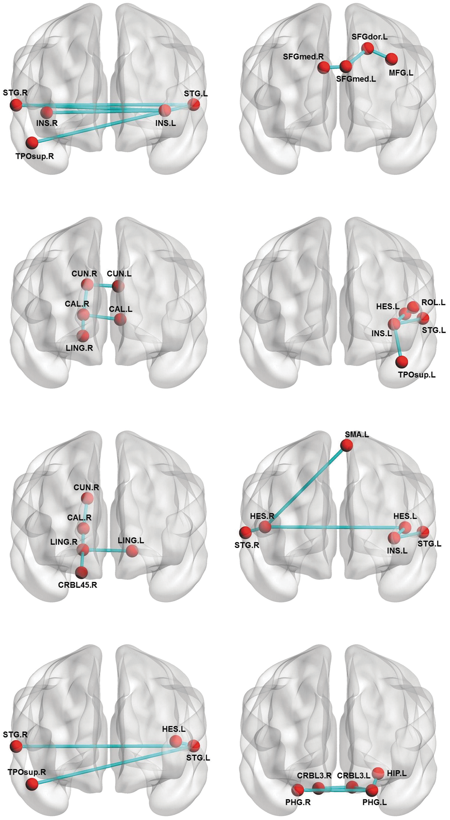
The discriminative subnetworks of healthy controls (the left column) and mild cognitive impairment (the right column). INS.L, left insula; INS.R, right insula; STG.L, left superior temporal gyri; STG.R, right superior temporal gyri; TPOsup.R, right superior temporal pole; TPOsup.L, left superior temporal pole; CUN.R, right cuneus; CUN.L, left cuneus; CAL.R, right calcarine sulcus; CAL.L, left calcarine sulcus; LING.R, right lingual gyrus; LING.L, left lingual gyrus; CRBL45.R, right lobule IV, V of cerebellar hemisphere; HES.R, right transverse temporal gyri; HES.L, left transverse temporal gyri; SFGmed.R, right superior frontal gyrus, medial part; SFGmed.L, left superior frontal gyrus, medial part; SFGdor.L, left superior frontal gyrus, dorsolateral; MFG.L, left middle frontal gyrus, lateral part; ROL.L, left rolandic operculum; SMA.L, left supplementary motor area; HIP.L, left hippocampus; PHG.L, left parahippocampal gyrus; PHG.R, right parahippocampal gyrus; CRBL3.L, left Lobule III of cerebellar hemisphere; CRBL.R, right Lobule III of cerebellar hemisphere. Figures were visualized using BrainNet Viewer (www.nitrc.org/projects/bnv/). Color images available online at www.liebertpub.com/brain

Discriminative regions

In this section, the authors count the number of occurrences of ROIs from all the mined discriminative subnetworks, and then choose the top 14 ROIs with the highest occurrences as the discriminative regions. Table 3 lists these top ranked ROIs, which are visually plotted in Figure 5. As can be seen from Table 3 and Figure 5, the discriminative regions include insula, calcarine sulcus, lingual gyrus, transverse temporal gyri, superior temporal gyrus, which are mostly related to vision, auditory processes, function of language, social cognition, and information processes.

FIG. 5.

Visual plot of the top 14 discriminative regions in Table 3. Color images available online at www.liebertpub.com/brain

Table 3.

Top 14 Discriminative Regions

Top 14 discriminative regions
L rolandic operculum
L insula
R insula
L calcarine sulcus
R calcarine sulcus
L lingual gyrus
R lingual gyrus
L transverse temporal gyri
R transverse temporal gyri
L superior temporal gyrus
R superior temporal gyrus
R superior temporal pole
L lobule IV, V of cerebellar hemisphere
R lobule IV, V of cerebellar hemisphere

L and R denote Left and Right, respectively.

Discussion

This article investigated the diagnostic power of discriminative subnetworks, which were mined from functional connectivity networks, derived from resting-state fMRI, for the identification of individuals with MCI from HC. The proposed method employed the frequent subgraph mining and graph kernel-based classification for functional connectivity networks-based MCI classification. The classification performance in the experimental results validated the effectiveness of this proposed method. Moreover, the proposed method also gains an inherent insight for better understanding pathology of the disease. Specifically, the authors analyze the connectivity of the selected discriminative subnetworks and find that MCI patients have a disrupted connectivity between regions related to vision, auditory, language, social cognition, and information processes, which is consistent with other existing studies. For example, (Wang et al., 2013) investigated the topological structure of the functional connectome in MCI patients and found an abnormal structure, as shown by impaired functional connectivity between different brain regions. On the other hand, the regions with high occurrence in discriminative subnetworks as discriminative regions are selected, which include insula, calcarine sulcus, lingual gyrus, transverse temporal gyri, and superior temporal gyrus reported to be related with AD/MCI disease in literature (Davatzikos et al., 2011; Grady et al., 2003; Han et al., 2011; Liu et al., 2011).

Overall, these results show that the proposed method can effectively identify the MCI patients from HC, and provide empirical evidence for disrupted local network organization in MCI at both the regional and connectional levels. Besides MCI classification, the authors further validate the efficacy of the proposed method for gender classification, as detailed in Appendix 2.

The effect of threshold

In AD/MCI studies, threshold-based methods have been widely used for exploring the topological properties of functional connectivity networks (Sanz-Arigita et al., 2010; Supekar et al., 2008). In functional network analysis, it is noteworthy that there is no golden rule to determine the choice of threshold. Therefore, many studies investigate their methods over a range of thresholds (Supekar et al., 2008; Zanin et al., 2012). In this study, for further investigating the stability of the proposed method, extra experiments using different thresholds are performed. First, this method is performed using all the five thresholds (i.e., 0.2, 0.3, 0.38, 0.4, and 0.45) used in the previous study (Jie et al., 2013b), and this method achieves classification accuracies of 89.2%, 97.3%, 94.6%, 91.9%, and 91.9%, respectively. In contrast, the method in (Jie et al., 2013b) obtained an ensemble classification accuracy of 91.9% by combining all these thresholds together, while the classification accuracies corresponding to individual thresholds are only 86.5%, 83.8%, 75.7%, 75.7%, and 64.9%, respectively. Moreover, the authors investigate the stability of this method under more delicate interval partition of thresholds, ranging from 0.2 to 0.4 with an increment of 0.02, and the corresponding results are shown in Figure 6. As can be seen from Figure 6, the performance curve is relatively stable with respect to different thresholds, which again validates the efficiency of the proposed method.

FIG. 6.

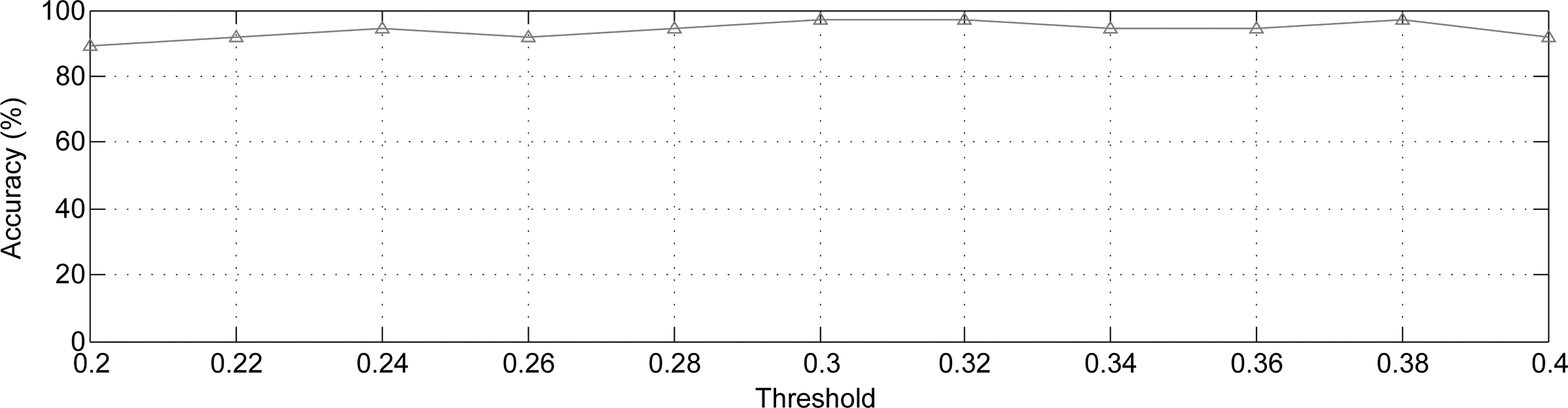
The classification performance curve with different thresholds.

The stability of the discriminative subnetworks

In this section, the authors computed the frequency of those mined discriminative subnetworks of the HC and MCI groups in Figure 4 in all 37 runs. The corresponding results (i.e., frequency) are (3/37, 37/37, 37/37, and 37/37) for HC (from top to bottom in Fig. 4) and (37/37, 2/37, 37/37, and 37/37) for MCI (from top to bottom in Fig. 4), respectively. This result suggests that most of the mined discriminative subnetworks of both the HC and MCI groups are stable. Especially, six discriminative subnetworks in Figure 4 (three for HC and three for MCI) have the frequency of 1, that is, appearing in all runs, showing a very high stability.

The choice of support parameter

In these experiments, the fixed values of support parameters for mining frequent subnetworks were used in each of the MCI and HC groups. Specifically, s=9/11 was used for the MCI group and s=22/24 was used for the HC group, respectively. In fact, other values for the support parameters were also used. However, because of the small sample size (and also the relatively large number of nodes (i.e., 116) in networks) of the training data (i.e., 11 for the MCI group and 24 for the HC group), smaller values of support (e.g., s=8/11 for the MCI group and 21/24 for the HC group) will lead to too many mined frequent subnetworks (usually over thousands), which are difficult for subsequent analysis. On the other hand, if larger values of support (e.g., s=10/11 for the MCI group and 23/24 for the HC group) are used, the mined frequent subnetworks will be too few (e.g., only 2 frequent subnetworks were mined for a certain run), which are insufficient for subsequent discrimination between MCI and HC. Actually, the authors computed the corresponding classification accuracy when using s=10/11 for the MCI group and 23/24 for the HC group, which is 81.08%. For this reason, in these experiments, the fixed values of s=9/11 for the MCI group and s=22/24 for the HC group were adopted, respectively.

Limitations

This study is limited by the following factors. First, during the network construction, the definition of nodes and edges is a critical step. Previous studies have demonstrated that network nodes can be defined using both anatomical and/or functional brain atlases and image voxels, but the constructed network exhibited significantly different topological properties (Hayasaka and Laurienti, 2010; He and Evans, 2010; Sanabria-Diaz et al., 2010; Wang et al., 2009). In the current study, following previous works (Jie et al., 2013a, 2013b, 2014), the authors adopted the widely used AAL template to parcellate the whole brain into 116 ROIs (including the cerebrum and cerebellar), and the correlation between ROIs is computed by the average time series of ROIs, which may cause intrinsic information being smoothed. One possible solution may be to use more delicate brain parcellation methods or using cortical landmarks (instead of average), for example, in (Zhu et al., 2013). However, this study does not analyze the impact of different brain parcellation atlases on the classification performance. Second, the performance of the proposed method may be affected by the unbalanced data. A classifier will normally try to adapt itself for better prediction of the class with majority. At present, the proposed method is not designed to handle this issue. Another limitation of the current study is the sample size of the material, which may reduce its generalization ability on MCI classification. In future, further evaluation of the proposed method on other brain diseases with larger size of subjects will be done, for example, ADHD (fcon_1000.projects.nitrc.org/indi/adhd200/index.html). Finally, the aim in this study is on individual classification rather than group analysis between HC and MCI, and thus, the authors did not put more focus on the possible neurobiological interpretations of this method.

Footnotes

Acknowledgment

The authors thank all the anonymous reviewers for their helpful comments, which improved the quality of the article. They thank Dr. Dinggang Shen for providing the MCI and the infant data sets used in the experiments. This work was supported by the Jiangsu Science Foundation for Distinguished Young Scholar under grant No. BK20130034, by the Specialized Research Fund for the Doctoral Program of Higher Education under grant No. 20123218110009, and also by the NUAA Fundamental Research Funds under grant No. NE2013105.

Author Disclosure Statement

No competing financial interests exist.

Appendices

References

Achard

, Bassett

, Meyer-Lindenberg

, Bullmore

. 2008. Fractal connectivity of long-memory networks. Phys Rev E Stat Nonlin Soft Matter Phys, 77:036104.

Alvarez

, Qi

, Yan

. 2011. A shortest-path graph kernel for estimating gene product semantic similarity. J Biomed Semantics, 2:3.

Bai

, Shu

, Yuan

, Shi

, Yu

, Wu

, Wang

, Xia

, He

, Zhang

. 2012. Topologically convergent and divergent structural connectivity patterns between patients with remitted geriatric depression and amnestic mild cognitive impairment. J Neurosci, 32:4307–4318.

Berchtold

, Cotman

. 1998. Evolution in the conceptualization of dementia and Alzheimer's disease: Greco-Roman period to the 1960s. Neurobiol Aging, 19:173–189.

Borgelt

, Berthold

. 2002. Mining Molecular Fragments: Finding Relevant Substructures of Molecules. Proceedings of the 2002 IEEE International Conference on Data Mining, Maebashi, Japan, pp. 51–58.

Borgwardt

, Ong

, Schonauer

, Vishwanathan

SVN

, Smola

, Kriegel

. 2005. Protein function prediction via graph kernels. Bioinformatics, 21:I47–I56.

Brookmeyer

, Johnson

, Ziegler-Graham

, Arrighi

. 2007. Forecasting the global burden of Alzheimer's disease. Alzheimers Dement, 3:186–191.

Busatto

, Garrido

, Almeida

, Castro

, Camargo

, Cid

, Buchpiguel

, Furuie

, Bottino

. 2003. A voxel-based morphometry study of temporal lobe gray matter reductions in Alzheimer's disease. Neurobiol Aging, 24:221–231.

Chen

, Ward

, Xie

, Li

, Wu

, Jones

, Franczak

, Antuono

, Li

. 2011. Classification of Alzheimer disease, mild cognitive impairment, and normal cognitive status with large-scale network analysis based on resting-state functional MR imaging. Radiology, 259:213–221.

10.

Chen

, He

, Rosa

, Germann

, Evans

. 2008. Revealing modular architecture of human brain structural networks by using cortical thickness from MRI. Cereb Cortex, 18:2374–2381.

11.

Cordes

, Haughton

, Arfanakis

, Carew

, Turski

, Moritz

, Quigley

, Meyerand

. 2001. Frequencies contributing to functional connectivity in the cerebral cortex in “esting-state” data. AJNR Am J Neuroradiol, 22:1326–1333.

12.

Cuingnet

, Gerardin

, Tessieras

, Auzias

, Lehericy

, Habert

, Chupin

, Benali

, Colliot

; Alzheimer's Disease Neuroimaging Initiative. 2011. Automatic classification of patients with Alzheimer's disease from structural MRI: a comparison of ten methods using the ADNI database. Neuroimage, 56:766–781.

13.

Davatzikos

, Bhatt

, Shaw

, Batmanghelich

, Trojanowski

. 2011. Prediction of MCI to AD conversion, via MRI, CSF biomarkers, and pattern classification. Neurobiol Aging, 32:2322.e2319–e2327.

14.

Davey

, Grayden

, Egan

, Johnston

. 2013. Filtering induces correlation in fMRI resting state data. Neuroimage, 64:728–740.

15.

Filippi

, Agosta

. 2011. Structural and functional network connectivity breakdown in Alzheimer's disease studied with magnetic resonance imaging techniques. J Alzheimers Dis, 24:455–474.

16.

Fornito

, Zalesky

, Bullmore

. 2010. Network scaling effects in graph analytic studies of human resting-state FMRI data. Front Syst Neurosci, 4:22.

17.

Gao

, Gilmore

, Giovanello

, Smith

, Shen

, Zhu

, Lin

. 2011. Temporal and spatial evolution of brain network topology during the first two years of life. PLoS One, 6:e25278.

18.

Gartner

, Flach

, Wrobel

. 2003. On graph kernels: hardness results and efficient alternatives. Learn Theory Kernel Machines, 2777:129–143.

19.

Gauthier

, Reisberg

, Zaudig

, Petersen

, Ritchie

, Broich

, Belleville

, Brodaty

, Bennett

, Chertkow

. 2006. Mild cognitive impairment. Lancet, 367:1262–1270.

20.

Gould

, Arroyo

, Brown

, Owen

, Bullmore

, Howard

. 2006. Brain mechanisms of successful compensation during learning in Alzheimer disease. Neurology, 67:1011–1017.

21.

Grady

, McIntosh

, Beig

, Keightley

, Burian

, Black

. 2003. Evidence from functional neuroimaging of a compensatory prefrontal network in Alzheimer's disease. J Neurosci, 23:986–993.

22.

Han

, Wang

, Zhao

, Min

, Lu

, Li

, He

, Jia

. 2011. Frequency-dependent changes in the amplitude of low-frequency fluctuations in amnestic mild cognitive impairment: a resting-state fMRI study. Neuroimage, 55:287–295.

23.

Harchaoui

, Bach

. 2007. Image Classification with Segmentation Graph Kernels. 2007 IEEE Conference on Computer Vision and Pattern Recognition, Minneapolis, Minnesota, USA, pp. 612–619.

24.

Hayasaka

, Laurienti

. 2010. Comparison of characteristics between region-and voxel-based network analyses in resting-state fMRI data. Neuroimage, 50:499–508.

25.

, Chen

, Evans

. 2007. Small-world anatomical networks in the human brain revealed by cortical thickness from MRI. Cereb Cortex, 17:2407–2419.

26.

, Evans

. 2010. Graph theoretical modeling of brain connectivity. Curr Opin Neurol, 23:341–350.

27.

Huan

, Wang

, Prins

. 2003. Efficient Mining of Frequent Subgraphs in the Presence of Isomorphism. Proceedings of the Third IEEE International Conference on Data Mining, Melbourne, Florida, USA, pp. 549–552.

28.

Huang

, Wahlund

, Dierks

, Julin

, Winblad

, Jelic

. 2000. Discrimination of Alzheimer's disease and mild cognitive impairment by equivalent EEG sources: a cross-sectional and longitudinal study. Clin Neurophysiol, 111:1961–1967.

29.

Inokuchi

, Washio

, Motoda

. 2000. An apriori-based algorithm for mining frequent substructures from graph data. Lect Notes Comput, 1910:13–23.

30.

Iturria-Medina

, Canales-Rodriguez

, Melie-Garcia

, Valdes-Hernandez

, Martinez-Montes

, Aleman-Gomez

, Sanchez-Bornot

. 2007. Characterizing brain anatomical connections using diffusion weighted MRI and graph theory. Neuroimage, 36:645–660.

31.

Jiang

, Coenen

, Zito

. 2013. A survey of frequent subgraph mining algorithms. Knowl Eng Rev, 28:75–105.

32.

Jie

, Zhang

, Gao

, Wang

, Wee

, Shen

. 2014. Integration of network topological and connectivity properties for neuroimaging classification. IEEE Trans Biomed Eng, 61:576–589.

33.

Jie

, Zhang

, Suk

, Wee

, Shen

. 2013a. Integrating multiple network properties for MCI identification. In: Wu

Guorong

, Zhang

Daoqiang

, Shen

Dinggang

, Yan

Pingkun

, Suzuki

Kenji

, Wang

Fei

(eds.), Machine Learning in Medical Imaging. Nagoya, Japan: Springer; pp. 9–16.

34.

Jie

, Zhang

, Wee

, Shen

. 2013b. Topological graph kernel on multiple thresholded functional connectivity networks for mild cognitive impairment classification. Hum Brain Mapp [Epub ahead of print]; DOI: 10.1002/hbm.22353.

35.

Kaiser

. 2011. A tutorial in connectome analysis: topological and spatial features of brain networks. Neuroimage, 57:892–907.

36.

Krishna

, Suri

NNRR

, Athithan

. 2011. A comparative survey of algorithms for frequent subgraph discovery. Curr Sci India, 100:190–198.

37.

Kuramochi

, Karypis

. 2004. An efficient algorithm for discovering frequent subgraphs. IEEE Trans Knowl Data Eng, 16:1038–1051.

38.

Liu

, Wang

, Yu

, He

, Zhou

, Liang

, Wang

, Jiang

. 2008. Regional homogeneity, functional connectivity and imaging markers of Alzheimer's disease: a review of resting-state fMRI studies. Neuropsychologia, 46:1648–1656.

39.

Liu

, Paajanen

, Zhang

, Westman

, Wahlund

, Simmons

, Tunnard

, Sobow

, Mecocci

, Tsolaki

, Vellas

, Muehlboeck

, Evans

, Spenger

, Lovestone

, Soininen

, Consortium

. 2011. Combination analysis of neuropsychological tests and structural MRI measures in differentiating AD, MCI and control groups—The AddNeuroMed study. Neurobiol Aging, 32:1198–1206.

40.

Mattsson

, Zetterberg

, Hansson

, Andreasen

, Parnetti

, Jonsson

, Herukka

, van der Flier

, Blankenstein

, Ewers

. 2009. CSF biomarkers and incipient Alzheimer disease in patients with mild cognitive impairment. JAMA, 302:385–393.

41.

McEvoy

, Fennema-Notestine

, Roddey

, Hagler

, Holland

, Karow

, Pung

, Brewer

, Dale

. 2009. Alzheimer disease: quantitative structural neuroimaging for detection and prediction of clinical and structural changes in mild cognitive impairment1. Radiology, 251:195–205.

42.

Morris

, Storandt

, Miller

, McKeel

, Price

, Rubin

, Berg

. 2001. Mild cognitive impairment represents early-stage Alzheimer disease. Arch Neurol, 58:397.

43.

Mosconi

, Tsui

, De Santi

, Li

, Rusinek

, Convit

, Li

, Boppana

, de Leon

. 2005. Reduced hippocampal metabolism in MCI and AD—automated FDG-PET image analysis. Neurology, 64:1860–1867.

44.

Petersen

, Doody

, Kurz

, Mohs

, Morris

, Rabins

, Ritchie

, Rossor

, Thal

, Winblad

. 2001. Current concepts in mild cognitive impairment. Arch Neurol, 58:1985–1992.

45.

Petrella

, Sheldon

, Prince

, Calhoun

, Doraiswamy

. 2011. Default mode network connectivity in stable vs progressive mild cognitive impairment. Neurology, 76:511–517.

46.

Richiardi

, Gschwind

, Simioni

, Annoni

, Greco

, Hagmann

, Schluep

, Vuilleumier

, Van De Ville

. 2012. Classifying minimally disabled multiple sclerosis patients from resting state functional connectivity. Neuroimage, 62:2021–2033.

47.

Robinson

, Hammers

, Ericsson

, Edwards

, Rueckert

. 2010. Identifying population differences in whole-brain structural networks: a machine learning approach. Neuroimage, 50:910–919.

48.

Rossini

, Del Percio

, Pasqualetti

, Cassetta

, Binetti

, Dal Forno

, Ferreri

, Frisoni

, Chiovenda

, Miniussi

, Parisi

, Tombini

, Vecchio

, Babiloni

. 2006. Conversion from mild cognitive impairment to Alzheimer's disease is predicted by sources and coherence of brain electroencephalography rhythms. Neuroscience, 143:793–803.

49.

Rubinov

, Sporns

. 2010. Complex network measures of brain connectivity: uses and interpretations. Neuroimage, 52:1059–1069.

50.

Sanabria-Diaz

, Melie-Garcia

, Iturria-Medina

, Aleman-Gomez

, Hernandez-Gonzalez

, Valdes-Urrutia

, Galan

, Valdes-Sosa

. 2010. Surface area and cortical thickness descriptors reveal different attributes of the structural human brain networks. Neuroimage, 50:1497–1510.

51.

Sanz-Arigita

, Schoonheim

, Damoiseaux

, Rombouts

SARB

, Maris

, Barkhof

, Scheltens

, Stam

. 2010. Loss of ‘small-world’ networks in Alzheimer's disease: graph analysis of fMRI resting-state functional connectivity. PLoS One, 5:e13788.

52.

Shaw

, Vanderstichele

, Knapik-Czajka

, Clark

, Aisen

, Petersen

, Blennow

, Soares

, Simon

, Lewczuk

. 2009. Cerebrospinal fluid biomarker signature in Alzheimer's disease neuroimaging initiative subjects. Ann Neurol, 65:403–413.

53.

Shen

, Davatzikos

. 2002. HAMMER: hierarchical attribute matching mechanism for elastic registration. IEEE Trans Med Imaging, 21:1421–1439.

54.

Shervashidze

, Schweitzer

, van Leeuwen

, Mehlhorn

, Borgwardt

. 2011. Weisfeiler-Lehman graph kernels. J Mach Learn Res, 12:2539–2561.

55.

Sperling

, Bates

, Chua

, Cocchiarella

, Rentz

, Rosen

, Schacter

, Albert

. 2003. fMRI studies of associative encoding in young and elderly controls and mild Alzheimer's disease. J Neurol Neurosurg Psychiatry, 74:44–50.

56.

Sporns

. 2012. From simple graphs to the connectome: networks in neuroimaging. Neuroimage, 62:881–886.

57.

Stam

, Jones

, Nolte

, Breakspear

, Scheltens

. 2007. Small-world networks and functional connectivity in Alzheimer's disease. Cereb Cortex, 17:92–99.

58.

Stephan

, Hilgetag

, Burns

GAPC

, O'Neill

, Young

, Kotter

. 2000. Computational analysis of functional connectivity between areas of primate cerebral cortex. Philos Trans R Soc B, 355:111–126.

59.

Stern

. 2006. Cognitive reserve and Alzheimer disease. Alzheimer Dis Assoc Disord, 20:S69–S74.

60.

Supekar

, Menon

, Rubin

, Musen

, Greicius

. 2008. Network analysis of intrinsic functional brain connectivity in Alzheimer's disease. PLoS Comput Biol, 4:e1000100.

61.

Tijms

, Wink

, de Haan

, van der Flier

, Stam

, Scheltens

, Barkhof

. 2013. Alzheimer's disease: connecting findings from graph theoretical studies of brain networks. Neurobiol Aging, 34:2023–2036.

62.

Tzourio-Mazoyer

, Landeau

, Papathanassiou

, Crivello

, Etard

, Delcroix

, Mazoyer

, Joliot

. 2002. Automated anatomical labeling of activations in SPM using a macroscopic anatomical parcellation of the MNI MRI single-subject brain. Neuroimage, 15:273–289.

63.

van den Heuvel

, Pol

HEH

. 2010. Exploring the brain network: A review on resting-state fMRI functional connectivity. Eur Neuropsychopharmacol, 20:519–534.

64.

van Wijk

, Stam

, Daffertshofer

. 2010. Comparing brain networks of different size and connectivity density using graph theory. PLoS One, 5:e13701.

65.

Vishwanathan

SVN

, Schraudolph

, Kondor

, Borgwardt

. 2010. Graph kernels. J Mach Learn Res, 11:1201–1242.

66.

Wang

, Wang

, Zang

, Yang

, Tang

, Gong

, Chen

, Zhu

, He

. 2009. Parcellation-dependent small-world brain functional networks: a resting-state fMRI study. Hum Brain Mapp, 30:1511–1523.

67.

Wang

, Zuo

, Dai

, Xia

, Zhao

, Jia

, Han

, He

. 2013. Disrupted functional brain connectome in individuals at risk for Alzheimer's disease. Biol Psychiatry, 73:472–481.

68.

Wang

, Jiang

, Liang

, Wang

, Tian

, Zhang

, Li

, Liu

. 2006. Discriminative analysis of early Alzheimer's disease based on two intrinsically anti-correlated networks with resting-state fMRI. Med Image Comput Comput Assist Interv, 9:340–347.

69.

Wang

, Liang

, Wang

, Tian

, Zhang

, Li

, Jiang

. 2007. Altered functional connectivity in early Alzheimer's disease: a resting-state fMRI study. Hum Brain Mapp, 28:967–978.

70.

Wee

, Yap

, Denny

, Browndyke

, Potter

, Welsh-Bohmer

, Wang

, Shen

. 2012a. Resting-state multi-spectrum functional connectivity networks for identification of MCI patients. PLoS One, 7:e37828.

71.

Wee

, Yap

, Li

, Denny

, Browndyke

, Potter

, Welsh-Bohmer

, Wang

, Shen

. 2011. Enriched white matter connectivity networks for accurate identification of MCI patients. Neuroimage, 54:1812–1822.

72.

Wee

, Yap

, Zhang

, Denny

, Browndyke

, Potter

, Welsh-Bohmer

, Wang

, Shen

. 2012b. Identification of MCI individuals using structural and functional connectivity networks. Neuroimage, 59:2045–2056.

73.

Xie

, He

. 2011. Mapping the Alzheimer's brain with connectomics. Front Psychiatry, 2:77.

74.

Yan

, Han

. 2002. gSpan: Graph-Based Substructure Pattern Mining. Proceedings of the 2002 IEEE International Conference on Data Mining, Maebashi, Japan, pp. 721–724.

75.

Zanin

, Sousa

, Papo

, Bajo

, Garcia-Prieto

, del Pozo

, Menasalvas

, Boccaletti

. 2012. Optimizing functional network representation of multivariate time series. Sci Rep, 2:630.

76.

Zhang

, Wang

, Zhou

, Yuan

, Shen

, Alzheimer's Disease Neuroimaging I. 2011. Multimodal classification of Alzheimer's disease and mild cognitive impairment. Neuroimage, 55:856–867.

77.

Zhou

, Wang

, Liu

, Ogunbona

, Shen

. 2013. Discriminative Brain Effective Connectivity Analysis for Alzheimer's Disease: A Kernel Learning Approach Upon Sprse Gaussian Bayesian network. 2013 IEEE Conference on Computer Vision and Pattern Recoginition. Portland, Oregon, USA.

78.

Zhou

, Wang

, Li

, Yap

, Shen

. 2011. Hierarchical anatomical brain networks for MCI prediction: revisiting volumetric measures. PLoS One, 6:e21935.

79.

Zhu

, Li

, Guo

, Jiang

, Zhang

, Chen

, Deng

, Faraco

, Jin

, Wee

, Yuan

, Lv

, Yin

, Hu

, Duan

, Hu

, Han

, Wang

, Shen

, Miller

, Li

, Liu

. 2013. DICCCOL: dense individualized and common connectivity-based cortical landmarks. Cereb Cortex, 23:786–800.

80.

Zuo

, Di Martino

, Kelly

, Shehzad

, Gee

, Klein

, Castellanos

, Biswal

, Milham

. 2010. The oscillating brain: complex and reliable. Neuroimage, 49:1432–1445.