Intrinsic Functional Component Analysis via Sparse Representation on Alzheimer's Disease Neuroimaging Initiative Database

Overview

As illustrated in Figure 1, the framework can be divided into three major parts: functional sparse representation (Fig. 1b, c), feature construction (Fig. 1f) based on learned dictionary matrix/coefficient weight matrix, and feature selection/classification (Fig. 1g). First, by using online dictionary learning methods, the whole-brain fMRI BOLD signals are sparsely represented as the product of common dictionary matrix (Fig. 1b) and the corresponding coefficient weight matrix (Fig. 1c). That is, the signals of each voxel can be sparsely and effectively represented as linear combinations of some atomic dictionary components. Through comparing with 10 predefined RSN templates, including visual, DMN, cerebellum, sensorimotor, auditory, executive control, and frontoparietal, we successfully identified highly similar dictionary atoms (Fig. 1d) from others (Fig. 1e) within each subject. Then for those identified dictionary atoms that are highly similar with the RSNs, the likelihood of being RSNs as well as the functional characteristics (e.g., functional connectivity) with other dictionary atoms are explored to construct multiple types of features (Fig. 1f). At last, all the features are fit in the correlation-based feature selection (CFS) algorithm and the ones with the most differentiation power will be preserved. An effective support vector machine (SVM) classifier was employed to solve the classification problem (Fig. 1g). In addition, those highly discriminating features are also analyzed and discussed in the “Results” section (Features with high differentiation power heading).

OPEN IN VIEWER

FIG. 1.

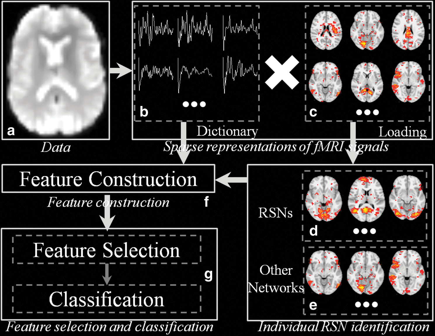
Illustration of the proposed framework. (a) Resting-state functional magnetic resonance imaging data. Here, the input dataset includes 210 subjects from the most recently updated ADNI database until September 2013. (b) Dictionary matrix. (c) Coefficient weight matrix. (d) Ten identified RSNs using ICA templates. (e) Other dictionary atoms. (f) Using dictionary matrix and identified RSNs we constructed six types of features. They are spatial overlapping rate, functional connectivity within RSNs, functional connectivity within dictionary, entropy of functional connectivity, entropy of component distribution within RSNs, and common dictionary distribution. (g) Correlation-based feature selection and support vector machine classifier. ADNI, Alzheimer's Disease Neuroimaging Initiative; ICA, independent-component analysis; RSN, resting-state network. Color images available online at www.liebertpub.com/brain

Data

The dataset used in the preparation of this article was obtained from the ADNI database (adni.loni.usc.edu). The ADNI was launched in 2003 by the National Institute on Aging (NIA), the National Institute of Biomedical Imaging and Bioengineering (NIBIB), the Food and Drug Administration (FDA), private pharmaceutical corporations, and nonprofit organizations, as a $60 million, 5-year public-private partnership. The primary goal of ADNI has been to test whether PET, serial MRI, other biological markers, and clinical and neuropsychological assessment can be combined to measure the progression of MCI and early AD. Determination of sensitive and specific markers of very early AD progression is intended to aid researchers and clinicians to develop new treatments and monitor their effectiveness, as well as lessen the time and cost of clinical trials. ADNI is the result of efforts of many coinvestigators from a broad range of academic institutions and private companies, and subjects have been recruited from over 50 sites across the United States and Canada. The initial goal of ADNI was to recruit 800 adults but which has been followed by ADNI-GO (2009) and ADNI-2 (2010). To date these three phases have recruited over 1500 subjects, ages from 55 to 90, to participate in the research, consisting of cognitively normal older individuals, people with early or LMCI, and people with early AD. For up-to-date information about ADNI database, see www.adni-info.org

Sparse representations of fMRI signals

Given a collection of data vectors \documentclass{aastex}\usepackage{amsbsy}\usepackage{amsfonts}\usepackage{amssymb}\usepackage{bm}\usepackage{mathrsfs}\usepackage{pifont}\usepackage{stmaryrd}\usepackage{textcomp}\usepackage{portland, xspace}\usepackage{amsmath, amsxtra}\pagestyle{empty}\DeclareMathSizes{10}{9}{7}{6}\begin{document}$$X = [ { \rm x}_1 , \ldots , { \rm x}_{ \rm n} ] \in {\mathbb R}^{{ \rm m} \times { \rm n}}$$ \end{document} , if there exists a linear combination of a small number of d_i that can effectively represent X, then we say that X admits a sparse approximation over dictionary D, where \documentclass{aastex}\usepackage{amsbsy}\usepackage{amsfonts}\usepackage{amssymb}\usepackage{bm}\usepackage{mathrsfs}\usepackage{pifont}\usepackage{stmaryrd}\usepackage{textcomp}\usepackage{portland, xspace}\usepackage{amsmath, amsxtra}\pagestyle{empty}\DeclareMathSizes{10}{9}{7}{6}\begin{document}$$D = [ { \rm d}_1 , \ldots , { \rm d}_{ \rm k} ] \in {\mathbb R}^{{ \rm m} \times { \rm k}}$$ \end{document} . A general form of cost function in sparse dictionary learning is defined as \documentclass{aastex}\usepackage{amsbsy}\usepackage{amsfonts}\usepackage{amssymb}\usepackage{bm}\usepackage{mathrsfs}\usepackage{pifont}\usepackage{stmaryrd}\usepackage{textcomp}\usepackage{portland, xspace}\usepackage{amsmath, amsxtra}\pagestyle{empty}\DeclareMathSizes{10}{9}{7}{6}\begin{document} \begin{align*}{\rm f_n} (D) = \frac {1} { \rm n } \sum _ { \rm i = 1}^{\rm n} \ell {\rm (x_i, D)}\tag {1}\end{align*} \end{document}

Where D \documentclass{aastex}\usepackage{amsbsy}\usepackage{amsfonts}\usepackage{amssymb}\usepackage{bm}\usepackage{mathrsfs}\usepackage{pifont}\usepackage{stmaryrd}\usepackage{textcomp}\usepackage{portland, xspace}\usepackage{amsmath, amsxtra}\pagestyle{empty}\DeclareMathSizes{10}{9}{7}{6}\begin{document}$$\in {\mathbb R}^{{ \rm m} \times { \rm k}}$$ \end{document} is the dictionary and ℓ is the loss function, which is to be small if D can effectively represent the original data X. In general, k will be much less than n.

In this article, for each R-fMRI dataset having n voxels with t time length, we are aiming to learn a neuroscience meaningful and over-complete dictionary \documentclass{aastex}\usepackage{amsbsy}\usepackage{amsfonts}\usepackage{amssymb}\usepackage{bm}\usepackage{mathrsfs}\usepackage{pifont}\usepackage{stmaryrd}\usepackage{textcomp}\usepackage{portland, xspace}\usepackage{amsmath, amsxtra}\pagestyle{empty}\DeclareMathSizes{10}{9}{7}{6}\begin{document}$${ \rm D} \in {\mathbb R}^{{ \rm t} \times { \rm m}}$$ \end{document} (m>t and m<< n) (Mairal et al., 2010) for the sparse representation of whole-brain signals, S. That is, for the R-fMRI signal set \documentclass{aastex}\usepackage{amsbsy}\usepackage{amsfonts}\usepackage{amssymb}\usepackage{bm}\usepackage{mathrsfs}\usepackage{pifont}\usepackage{stmaryrd}\usepackage{textcomp}\usepackage{portland, xspace}\usepackage{amsmath, amsxtra}\pagestyle{empty}\DeclareMathSizes{10}{9}{7}{6}\begin{document}$$S = [ s_1 , s_2 , \ldots s_n ] \in {\mathbb R}^{{ \rm t} \times { \rm n}}$$ \end{document} , the empirical cost function is rewritten as Equation (2) by considering the average loss of regression of n signals. \documentclass{aastex}\usepackage{amsbsy}\usepackage{amsfonts}\usepackage{amssymb}\usepackage{bm}\usepackage{mathrsfs}\usepackage{pifont}\usepackage{stmaryrd}\usepackage{textcomp}\usepackage{portland, xspace}\usepackage{amsmath, amsxtra}\pagestyle{empty}\DeclareMathSizes{10}{9}{7}{6}\begin{document} \begin{align*}{ \rm f } _ { \rm n } ( { \rm D } ) { { \Delta \atop= } } \frac { 1 } { { \rm n } } \sum_ { \rm i = 1 } ^ { \rm n } \ell ( { \rm s } _ { \rm i } , { \rm D } ) \tag { 2 } \end{align*}\end{document}

For an effective sparse representation using D, the general loss function is further defined in Equation (3) by using a ℓ₁ regularization that yields to a sparse resolution of α_i. Similar to LASSO (Tibshirani, 1996), here λ is a regularization parameter that can be used as a trade-off item between the sparsity level and the regression residual. \documentclass{aastex}\usepackage{amsbsy}\usepackage{amsfonts}\usepackage{amssymb}\usepackage{bm}\usepackage{mathrsfs}\usepackage{pifont}\usepackage{stmaryrd}\usepackage{textcomp}\usepackage{portland, xspace}\usepackage{amsmath, amsxtra}\pagestyle{empty}\DeclareMathSizes{10}{9}{7}{6}\begin{document} \begin{align*}\ell ( { \rm s } _ { \rm i } , { \rm D } ) { {\Delta \atop= } } \min \nolimits_ { \alpha_ { \rm i } \in { \mathbb R } } { \rm m } \frac { 1 } { 2 } \mid \mid { \rm s } _ {\rm i } - { \rm D } \alpha_ { \rm i } \mid \mid _2^2 + \lambda \mid \mid \alpha_ { \rm i } \mid \mid _1 \tag { 3 } \end{align*}\end{document}

Because we are more interested with the fluctuation shapes and patterns of basis fMRI BOLD activities, it is necessary to avoid D having an arbitrarily large number of elements. So the columns \documentclass{aastex}\usepackage{amsbsy}\usepackage{amsfonts}\usepackage{amssymb}\usepackage{bm}\usepackage{mathrsfs}\usepackage{pifont}\usepackage{stmaryrd}\usepackage{textcomp}\usepackage{portland, xspace}\usepackage{amsmath, amsxtra}\pagestyle{empty}\DeclareMathSizes{10}{9}{7}{6}\begin{document}$${ \rm d}_1 , { \rm d}_2 , \ldots \ \ldots { \rm d}_{ \rm m}$$ \end{document} in the learned dictionary D are constrained by Equation (4). \documentclass{aastex}\usepackage{amsbsy}\usepackage{amsfonts}\usepackage{amssymb}\usepackage{bm}\usepackage{mathrsfs}\usepackage{pifont}\usepackage{stmaryrd}\usepackage{textcomp}\usepackage{portland, xspace}\usepackage{amsmath, amsxtra}\pagestyle{empty}\DeclareMathSizes{10}{9}{7}{6}\begin{document} \begin{align*}C {{ \Delta \atop= }} \{ { \rm D} \in{\mathbb R}^{{ \rm t} \times { \rm m}} \ { \rm s}.{ \rm t}. \ \forall { \rm j} = 1 , \ldots { \rm m} , \, { \rm d}_{ \rm j}^{ \rm T} { \rm d}_{ \rm j} \leq 1 \} \tag{4}\end{align*} \end{document}

Eventually, the whole solution of dictionary learning problem in this article can be rewritten as a matrix factorization with ℓ₁ regulation in Equation (5). \documentclass{aastex}\usepackage{amsbsy}\usepackage{amsfonts}\usepackage{amssymb}\usepackage{bm}\usepackage{mathrsfs}\usepackage{pifont}\usepackage{stmaryrd}\usepackage{textcomp}\usepackage{portland, xspace}\usepackage{amsmath, amsxtra}\pagestyle{empty}\DeclareMathSizes{10}{9}{7}{6}\begin{document} \begin{align*}\min \nolimits_ { D \epsilon C , \alpha_ { \rm i} \in { { \mathbb R } } ^ { \rm m } } \frac { 1 } { 2 } \mid \mid{ \rm s } _ { \rm i } - D \alpha_ { \rm i } \mid \mid _2^2 + \lambda \mid \mid \alpha_ { \rm i } \mid \mid _1 \tag { 5 } \end{align*} \end{document}

Specifically, the sparse learning procedure in this article includes three steps. First, for each single-subject's brain, we extract preprocessed R-fMRI signals of whole brain by using individual brain mask. Then, after normalizing the signal to have zero mean and standard deviation of 1, these signals are reassembled into a big matrix S \documentclass{aastex}\usepackage{amsbsy}\usepackage{amsfonts}\usepackage{amssymb}\usepackage{bm}\usepackage{mathrsfs}\usepackage{pifont}\usepackage{stmaryrd}\usepackage{textcomp}\usepackage{portland, xspace}\usepackage{amsmath, amsxtra}\pagestyle{empty}\DeclareMathSizes{10}{9}{7}{6}\begin{document}$$\in {\mathbb R}^{{ \rm t} \times { \rm n}}$$ \end{document} , where t is the number of time points (fMRI volume numbers) and n columns represent fMRI signals extracted from n GM voxels. Finally, by applying a publicly available efficient online dictionary learning methods (Mairal et al., 2010), each fMRI signal (each column vector) in S can be modeled as a linear combination of a small size of learned dictionary atoms. For example, a specific signal vector, s_i , can be represented as the product of basis dictionary D and α_i , where α_i is the corresponding coefficient vector in the coefficient weight matrix.

The rationale and advantages behind using sparse representation of fMRI signals have two aspects. (1) As mentioned in the “Introduction” part, from neuroscience perspective, it has been widely agreed that a variety of brain networks and regions exhibit strong functional heterogeneity and diversity (Anderson et al., 2013; Duncan, 2010; Fedorenko et al., 2013; Kanwisher, 2010; Pessoa, 2012). That is, the same brain region could participate in multiple functional processes/domains simultaneously and a single functional network might recruit various neuroanatomic areas at different stages as well. So the practical fMRI signals of every single voxel tend to reflect a complex functional activity resulting from multiple components/sources within the whole brain. Under this case, a natural strategy is to decompose the actual signals back to multiple components that potentially represent the original sources. Here, we adopted the same assumption as previous studies (Lee et al., 2011; Oikonomou et al., 2012) that the components of each voxel's fMRI signal are sparse and the neural integration of those components is linear. (2) Given the fact that it is largely unknown to what extent those multiple interacting functional networks spatially overlap with each other and jointly fulfill the intact brain functions, we do not enforce the statistically independent constraint to the decomposed components like independent component analysis (ICA) (Calhoun et al., 2001) does. Therefore, our framework has more freedom during the sparse learning procedure and eliminates the need for initialization using a predefined model at the most extent.

Individual RSN identification

As described in “Sparse representations of fMRI signals” heading and illustrated in Figure 1, for each atom in the dictionary D, the corresponding coefficient vector α_i of the coefficient weight matrix can be projected back to the volumetric fMRI image space for the interpretation of the spatial patterns. In this way, the spatial patterns of atoms in different subjects can be compared within a template image space to determine their spatial correspondences, as well as to further identify meaningful RSNs within each subject.

In R-fMRI data analysis, a meaningful RSN is identified and examined mainly based on its spatial pattern, since the temporal and frequency characteristics have not been fully understood or quantitatively described. Specifically, in this article, a spatial-pattern-overlapping metric is adopted to identify meaningful RSNs in each subject and defined as \documentclass{aastex}\usepackage{amsbsy}\usepackage{amsfonts}\usepackage{amssymb}\usepackage{bm}\usepackage{mathrsfs}\usepackage{pifont}\usepackage{stmaryrd}\usepackage{textcomp}\usepackage{portland, xspace}\usepackage{amsmath, amsxtra}\pagestyle{empty}\DeclareMathSizes{10}{9}{7}{6}\begin{document} \begin{align*} { \rm SOR } ( { \rm X , T } ) = \frac { \mid { \rm X } \cap { \rm T } \mid } { \mid { \rm T } \mid } \tag { 6 } \end{align*} \end{document}

Where X is the spatial pattern of one functional component, T is a specific RSN template, and SOR is the spatial overlapping rate of X and T. For each subject, we first calculated the SORs of all spatial patterns contained in the coefficient weight matrix with a specific RSN template, and sorted them in decreased order. Then the first spatial pattern with the highest SOR (Fig. 1d) was determined as the specific RSN of this subject. Moreover, the corresponding atoms of the spatial patterns were used for feature construction, which will be detailed in the following heading. In this article, we adopted the 10 well-defined and widely known RSNs in Smith and coworkers (2009) as the RSN templates to identify the corresponding RSNs in each subject. More details of the 10 RSN templates are illustrated in “RSN identification” heading.

Feature construction

After the sparse representation of fMRI signals and identification of 10 RSNs, we constructed six types of features that can effectively reflect both spatial and functional characteristics during the resting state. They are SOR, functional connectivity within RSNs (FC-RSNs), functional connectivity within dictionary (FC-D), entropy of functional connectivity (ET-FC), entropy of component distribution within RSNs (ET-CDRSNs), and common dictionary distribution (CDC). Except for the first type of feature (SOR), the other five are directly or indirectly derived from the dictionary matrix.

Feature selection and classification

So far we have six types of features and we are aiming to preserve only those features with most differentiation power. At the same time we also need to consider the relevance among different features since sometimes a set of “good” features cannot predict well when only part of them are used. In this article we employed the CFS (Hall and Smith, 1999) algorithm as the feature selection strategy. Briefly, the core idea of CFS is that through a heuristic process it evaluates the merit of a subset of all the features by considering the “goodness” of individual ones along with the intercorrelation among them when predicting. That is, CFS will calculate feature-class and feature-feature correlations at the same time. Given a subset of features, S, with k features, the Merit_s is defined as: \documentclass{aastex}\usepackage{amsbsy}\usepackage{amsfonts}\usepackage{amssymb}\usepackage{bm}\usepackage{mathrsfs}\usepackage{pifont}\usepackage{stmaryrd}\usepackage{textcomp}\usepackage{portland, xspace}\usepackage{amsmath, amsxtra}\pagestyle{empty}\DeclareMathSizes{10}{9}{7}{6}\begin{document} \begin{align*} {\rm Merit}_{\rm s} = \frac {{\rm k}{\overline{\rm Corre (c , f)}}} {\sqrt {{\rm k} + ({\rm k} - 1)} {\overline{\rm Corre (f , f)}}} \tag {7} \end{align*}\end{document}

Where \documentclass{aastex}\usepackage{amsbsy}\usepackage{amsfonts}\usepackage{amssymb}\usepackage{bm}\usepackage{mathrsfs}\usepackage{pifont}\usepackage{stmaryrd}\usepackage{textcomp}\usepackage{portland, xspace}\usepackage{amsmath, amsxtra}\pagestyle{empty}\DeclareMathSizes{10}{9}{7}{6}\begin{document}$$\overline{{ \rm Corre ( c , f ) }}$$ \end{document} and \documentclass{aastex}\usepackage{amsbsy}\usepackage{amsfonts}\usepackage{amssymb}\usepackage{bm}\usepackage{mathrsfs}\usepackage{pifont}\usepackage{stmaryrd}\usepackage{textcomp}\usepackage{portland, xspace}\usepackage{amsmath, amsxtra}\pagestyle{empty}\DeclareMathSizes{10}{9}{7}{6}\begin{document}$$\overline{{ \rm Corre ( f , f ) }}$$ \end{document} represent mean feature-class correlation and average feature-feature intercorrelation, respectively. Here we adopted Pearson correlation coefficient as the measurement for the correlation. Corre(c, f) and Corre(f, f) are defined as Corre(c, f)=cov(c, f)/σ_cσ_f and Corre(f, f)=cov(f_i , f_j )/σ_fi σ_fj , where f_i and f_j are two different features, cov(.) is the covariance, and σ is the standard deviation. Once we obtained the most discriminative features following CFS procedure; an SVM classifier (Chang and Lin, 2001) was employed for solving the classification problem. Specifically, for each group, a 10-fold cross-validation was adopted to evaluate the performance of classifiers with different parameters. The major parameters include type of SVM (C-SVC and nu-SVC), kernel function type (linear, polynomial, radial basis function, and sigmoid), and penalty parameter C (ranges from 2⁻¹⁰ to 2¹⁰, interval is 2^0.1). For each of all combinations of those parameters, we used 10-fold cross-validation to obtain the classification accuracy, respectively. Then, the parameter sets with highest classification accuracy are obtained. In total, we have trained five classifiers (NC/AD, NC/SMC, NC/EMCI, NC/LMCI, and NC/EMCI+LMCI). The detailed classification results including sensitivity (proportion of patients correctly predicted) and specificity (proportion of healthy controls correctly predicted) are showed in “Classification results based on sparse representation features” heading.

RSN identification

As described in “Individual RSN identification” heading, we adopted 10 well-defined RSN templates provided in http://fsl.fmrib.ox.ac.uk/analysis/brainmap+rsns/ (Smith et al., 2009) to identify the corresponding 10 RSNs in each subject. The first row of Figure 2 shows the most informative slice as the spatial pattern of each RSN template. In brief, RSNs#1, #2, and #3 are located in the “visual” cortex, and include medial (BA 17), occipital pole, and lateral visual areas (BAs 18/19), respectively. RSN #4 is known as the “default mode network” (DMN) (Raichle et al., 2001), which mainly includes anterior (BAs 12/32) and posterior cingulate cortex (BA 29), the medial prefrontal gyrus (BAs 9/10/11), and bilateral supramarginal gyrus (BA 39). RSN #5 is located in cerebellum. RSN #6 is known as the “sensorimotor” network, which mainly includes pre- and postcentral gyrus (BAs 1/2/3/4), and the supplementary motor area (BA 6). RSN #7, known as the “auditory” system, encompasses the Heschl's gyrus, lateral superior temporal gyrus, and posterior insular cortex. RSN #8 includes anterior cingulate and paracingulate regions and is known as “executive control” network. RSNs #9 and #10 show networks that have strong lateralization in the right (RSN #9) and left (RSN #10) hemispheres, covering the middle frontal and orbital (BAs 6/9/10) and superior parietal areas (BAs 7/40). More details of the 10 RSNs are referred to Smith and coworkers (2009).

OPEN IN VIEWER

FIG. 2.

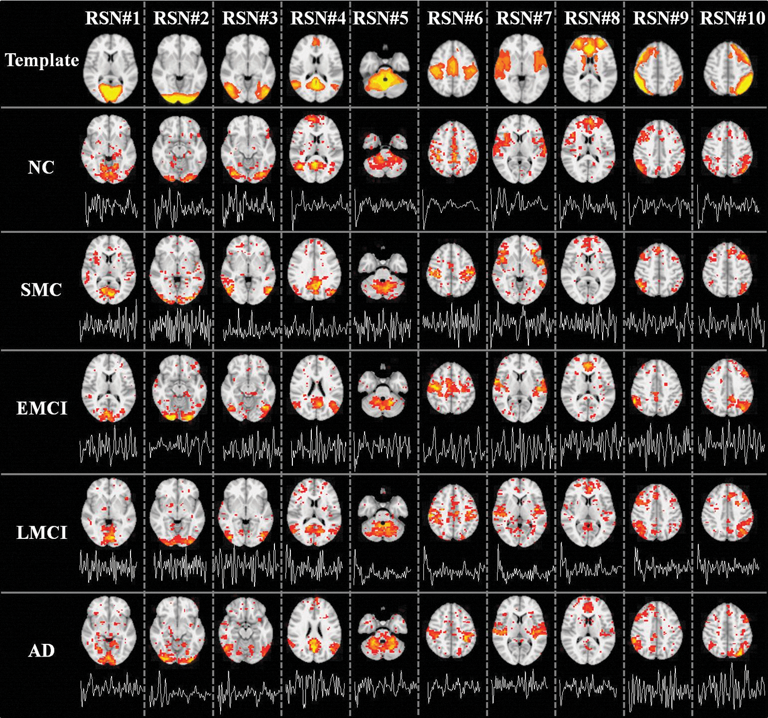
Ten well-matched RSNs identified from sparse representation. The first row showed the 10 RSN templates. For each template, the most informative slice, which is superimposed on the MNI152 template image, was shown as the spatial pattern. Rows 2 to 6 show the identified RSNs of a randomly selected subject of five groups (NC, SMC, EMCI, LMCI, and AD), respectively. In each subfigure, the most informative slice, superimposed on the MNI152 template image, was shown as the spatial pattern of a specific RSN. The time series of corresponding atom was also shown below each spatial pattern of the RSN. All 10 RSNs were matched by calculating and sorting the overlapping rate with the corresponding RSN templates (first row) provided in http://fsl.fmrib.ox.ac.uk/analysis/brainmap+rsns/ (Smith et al., 2009). The RSN templates shown in first row were thresholded at z=3. The color scale of spatial maps in sparse representation ranges from 0.1 to 10. AD, Alzheimer's disease; EMCI, early mild cognitive impairment; LMCI, late mild cognitive impairment; SMC, significant memory concern. Color images available online at www.liebertpub.com/brain

As illustrated in “Imaging data acquisition and data preprocessing” and “Sparse representations of fMRI signals” headings, since the time points t=140 for each subject, we set the dictionary size m>140 based on our experience to learn an over-complete (m>t) dictionary D and corresponding coefficient weight matrix α for each subject. Afterward, 10 RSNs were identified for each subject in all five groups (NC, SMC, EMCI, LMCI, and AD) via the method in “Individual RSN identification” heading. Note that to evaluate the impact of parameter selection, different combinations of parameters were explored to verify whether reproducible and consistent results can be achieved. Specifically, the dictionary learning and sparse representation pipeline was applied to subjects of NC group with different combinations of parameters since we expect to exclude the possible effect of diseased group. To make fair and easy comparison, first, λ is fixed, and we change the dictionary size from 200 to 600 (interval is 100). The mean overlap rate of all identified RSNs in all subjects is 0.38, 0.30, 0.31, 0.24, and 0.23. Second, m is fixed and λ changes from 1.0 to 2.0 (interval is 0.5). The mean overlap rate of all identified RSNs in all subjects is 0.31, 0.31, and 0.24. From the comparison, we can see that although the parameter alteration will cause slight spatial variation for the derived RSNs, the overall spatial overlap rate is reasonably stable. In this article, we chose m=200 and λ=1.5 with better spatial overlap rate of RSN in NC group. Rows 2 to 6 of Figure 2 show the 10 identified well-matched RSNs of a randomly selected subject in each of the five groups, respectively. In each subfigure, the most informative slice, superimposed on the MNI152 template image, was shown as the spatial pattern of a specific RSN. The time series of corresponding atom was also shown below each spatial pattern. Quantitatively, the mean overlap rate of all 10 RSNs is 0.38 (0.24 to 0.52) for all subjects in NC group, 0.37 (0.25 to 0.49) for SMC group, 0.37 (0.25 to 0.48) for EMCI group, 0.34 (0.23 to 0.44) for LMCI group, and 0.34 (0.24 to 0.46) for AD group. More detailed results are shown in Table 1. We can see that for some specific RSNs (e.g., RSN #4 representing DMN), the mean overlap rate is different across the five groups and the trend is decreasing along with the disease progression (from 0.52 in NC to 0.46 in AD for RSN #4, as detailed in Table 1), demonstrating that the overlap rate might be an effective feature to differentiate subjects between two groups.

Classification results based on sparse representation features

In this section, we constructed six types of features (SOR, FC-RSNs, FC-D, ET-FC, ET-CDRSNs, and CDC) containing both spatial and functional characteristics of R-fMRI data illustrated in “Feature construction” heading, and performed classification based on these features. For the feature construction, it should be noted that, in “Individual RSN identification” heading, we calculated the SORs of all spatial patterns of atoms with a specific RSN template, and sorted them in decreasing order. It is highly possible that first several spatial patterns may have similar high SOR with a specific RSN template. As a consequence, for each RSN, we considered top five spatial patterns with highest SOR and adopted the corresponding atoms to measure functional characteristics and construct features. Our rationale of considering top five spatial patterns for each RSN is twofold. (1) There might be intrinsic functional characteristics missed to differentiate normal controls from patients if we only chose top one spatial pattern merely based on SOR criterion. (2) The potential feature redundancy problem of introducing top five spatial patterns for each RSN can be effectively solved in the feature selection step via CFS. Finally, the numbers of features in each type are listed as following: 10 for SOR; 45×5=225 for FC-RSNs; 10×5=50 for FC-D, ET-FC, and ET-CDRSNs, respectively; and 200 for CDC. The total number of features is 585 for each subject. CFS was then adopted on all 585 features of subjects in each group pair (NC/AD, NC/SMC, NC/EMCI, NC/LMCI, and NC/EMCI+LMCI) to perform feature selection. Finally 10-fold cross-validation was performed for classification of each group pair via SVM.

We summarized the number of features before and after CFS and the corresponding classification results in Table 2. If we trained classifiers and performed classification using all 585 features, then the classification accuracy is not satisfied for all five group pairs (40.38% to 67.00%). After CFS, 5 to 30 features survived for the five group pairs detailed in Table 2. We can see that with the most relevant and discriminative features, the classification accuracy substantially improved for all five group pairs (80.00% to 94.12%). Moreover, we removed the eight subjects in EMCI group with different TR (not 3 sec) to exclude the potential effect of the scan parameters, and performed the feature selection and classification. The classification accuracy is 79.59%, specificity is 72.00%, and sensitivity is 87.50%. The results did not change much compared with the results in Table 2. We will interpret those features with high differentiation power in detail in the following heading.

Features with high differentiation power

As illustrated in “Classification results based on sparse representation features” heading, we adopted CFS to obtain the features with high differentiation power for each group pair. Table 3 summarized the detailed feature numbers in six feature types after CFS for each group pair. We discuss the features with high differentiation in each of the five group pairs in detail as follows.

For NC-SMC group, there are 22 features in total after CFS. Specifically, there is no feature in SOR type. For FC-RSNs type, there are 13 features, including the functional connectivity between RSNs #4–#10, #5–#8, #1–#3, #3–#6, #3–#7, #7–#8, #1–#8, #3–#4, #4–#7, #1–#4, and #4–#5. The RSN IDs can be referred to Figure 2. This result indicates that there are widespread functional connectivity alterations among RSNs in SMC. For FC-D type, there are two features related to RSNs #1 and #8. There is one feature in ET-FC that corresponds to RSN #8. For ET-CDRSNs type, there are three features related to RSNs #1 and #5. For CDC, there are three features representing the common atoms #97, #133, and #179. The time series of these common atoms with high differentiation power are shown in Figure 3.

OPEN IN VIEWER

FIG. 3.

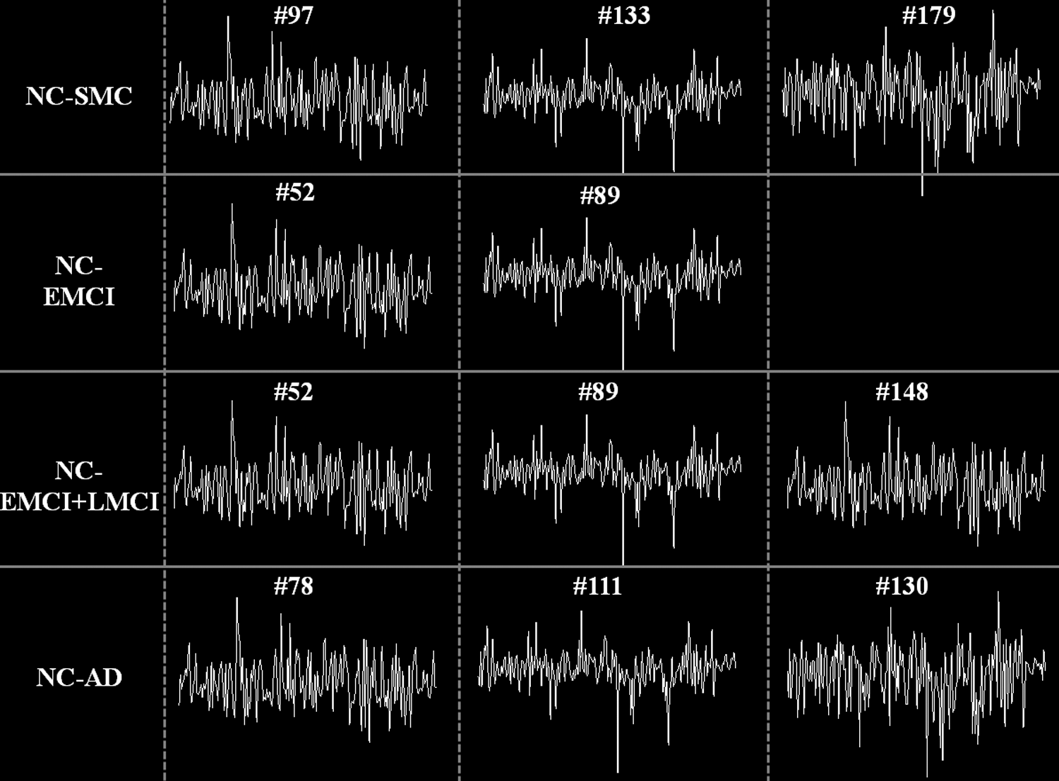
Time series of the common atoms with high differentiation power in each group pair. There are 140 time points. The index of the common atoms in the learned dictionary for each subject is shown above the time series of the atoms.

For NC-EMCI group, there are eight features in total after CFS. There is one feature in SOR type corresponding to RSN #1. For FC-RSNs type, there are two features corresponding to the functional connectivity between RSNs #3–#5 and #5–#6. For FC-D type, there is one feature corresponding to RSN #4. For ET-FC type, there is one feature corresponding to RSN #1. For ET-CDRSNs type, one feature corresponds to RSN #3. For CDC, two features correspond to atoms #52 and #89 (Fig. 3).

For NC-LMCI group, there are five features in total. There is no feature in SOR, ET-FC, or CDC type. For FC-RSNs type, there are two features corresponding to the functional connectivity between RSNs #1–#4 and #4–#5. For FC-D type, there are two features corresponding to RSNs #2 and #4. There is one feature in ET-CDRSNs corresponding to RSN #10. We can see that RSN #4, known as DMN, has discriminative functional characteristics in differentiating LMCI from NC.

For NC-EMCI+LMCI group, there are 30 features in total after CFS. There is one feature in SOR corresponding to RSN #2. For FC-RSNs, there are 17 features corresponding to the functional connectivity between RSNs #2–#8, #5–#10, #7–#10, #2–#9, #4–#7, #1–#6, #3–#5, #4–#5, #4–#7, #6–#8, #1–#4, #1–#10, #2–#4, #3–#10, #5–#6, and #6–#9. This result is in agreement with our previous results that show that there are widespread functional connectivity alterations among RSNs in MCI (Jiang et al., 2013). For FC-D type, there are four features related to RSNs #4, #6, and #7. For ET-FC, there are two features corresponding to RSNs #4 and #3. There are three features in ET-CDRSNs corresponding to RSNs #2, #3, and #4. For CDC type, there are three features corresponding to atoms #52, #89, and #148 (Fig. 3). We can also see that RSN #4, known as DMN, has discriminative functional characteristics in differentiating MCI from NC. It should be noted that the performance of NC/EMCI+LMCI group classification is better than NC/EMCI and NC/LMCI. Although we cannot compare the classification results of the three groups directly since the classifiers of the three groups were trained separately based on different and specific features of the three groups after feature selection, from theoretical perspective, one possible explanation is that after feature selection, more features that have relevant and discriminative power for classification were retained in the NC/EMCI+LMCI group than those in NC/EMCI and NC/LMCI groups.

For NC-AD group, there are 11 features in total after CFS. There are three features in SOR type corresponding to RSNs #1, #2, and #4. For FC-RSNs, there are three features corresponding to the functional connectivity between RSNs #3–#8, #4–#8, and #7–#9. There is no feature in FC-D type. For ET-FC type, there is one feature corresponding to RSN #1. For ET-CDRSNs type, there is one feature corresponding to RSN #10. For CDC type, there are three features corresponding to atoms #78, #111, and #130 (Fig. 3).