Connectomic Profiles for Individualized Resting State Networks and Regions of Interest

Abstract

Functional connectivity analysis of human brain resting state functional magnetic resonance imaging (rsfMRI) data and resultant functional networks, or RSNs, have drawn increasing interest in both research and clinical applications. A fundamental yet challenging problem is to identify distinct functional regions or regions of interest (ROIs) that have accurate functional correspondence across subjects. This article presents an algorithmic framework to identify ROIs of common RSNs at the individual level. It first employed a dual-sparsity dictionary learning algorithm to extract group connectomic profiles of ROIs and RSNs from noisy and high-dimensional fMRI data, with special attention to the well-known inter-subject variability in anatomy and then identified the ROIs of a given individual by employing both anatomic and group connectomic profile constraints using an energy minimization approach. Applications of this framework demonstrated that it can identify individualized ROIs of RSNs with superior performance over commonly used registration methods in terms of functional correspondence, and a test–retest study revealed that the framework is robust and consistent across both short-interval and long-interval repeated sessions of the same population. These results indicate that our framework can provide accurate substrates for individualized rsfMRI analysis.

Introduction

Functional connectivity (FC) analysis of resting state functional magnetic resonance imaging (rsfMRI) data and resultant functional networks (RSNs) have drawn increasing interest in both basic and clinical neuroscience. For instance, as one of the most widely studied RSNs, the default mode network (DMN) has been extensively examined using multiple imaging modalities, including positron emission tomography (PET) (Gusnard et al., 2001), fMRI (Greicius et al., 2003), magnetoencephalography (MEG) (Brookes et al., 2011), and intracranial recordings (Dastjerdi et al., 2011). Clinically, altered FC in DMN has been found in neuropsychiatric and neurological disorders, including autism (Kennedy et al., 2006), schizophrenia (Bluhm et al., 2007), and Alzheimer's disease (Greicius et al., 2004). The methods used to map FC networks can be broadly divided into two categories: model-based (e.g., seed-based univariate analysis), data-driven [e.g., independent component analysis (ICA), and graph-based clustering analysis]. A review of these methods is beyond the scope of this work, but can be found in several recent articles (Calhoun et al., 2009).

A fundamental yet challenging problem in FC analysis is to identify regions of interest (ROIs) that have accurate functional correspondence across individuals (Liu, 2011; Varoquaux and Craddock, 2013). It is reported that inaccurate ROIs in fMRI studies may seriously confound the identification of brain networks (Smith et al., 2011). The barriers to achieving accurate functional correspondence across subjects are at least twofold. (1) Huge anatomical variability exists across individuals, making it almost impossible to achieve anatomical correspondence at the voxel level through image registration (Li et al., 2012a; Ng et al., 2012; Roland et al., 1997; Zhu et al., 2013). For example, our study using task-based fMRI demonstrated that ROIs derived from state-of-the-art registration algorithms can easily deviate from the ground truth by 10 mm, no matter which algorithm was used, linear or nonlinear (Li et al., 2012a; Zhu et al., 2013). Unfortunately, to obtain group analysis results to infer individual counterparts, the fMRI community relies heavily on spatial smoothing and image registration, which inevitably affect the group connectomic profiles of functional ROIs and degrade the accuracy of ROI localization at the individual level. (2) Spontaneous fluctuation changes due to internal cognitive and/or perceptional processes are often marred by other non-neuronal sources, including physiological fluctuations such as cardiac or respiratory activity (Chang and Glover, 2010; Lund et al., 2006). As such, the connectomic profile of a functional ROI may be contaminated by these non-neuronal fluctuations.

Recently, there have been multiple studies aiming to build ROIs/RSNs correspondence across subjects based on fMRI data. For instance, Thirion and colleagues (2006) introduced a two-step procedure for task-based fMRI analysis to deal with the shortcomings of spatial normalization. They first performed intra-subject spectral clustering to delineate homogeneous and connected regions, and subsequently obtained group parcels that are spatially coherent and functionally homogeneous across subjects through a hierarchical approach. Similarly, Naveau and colleagues (2012) applied multi-scale clustering on individual ICA maps to build RSN correspondence across subjects. Blumensath and colleagues (2013) also adopted a similar strategy to parcellate the brain using rsfMRI. They generated a large number of initial individual ROIs based on local stability and then built a parcellation tree through hierarchical clustering. The correspondences across parcellations were determined based on Dice's coefficient. Different from the above-mentioned studies, Varoquaux and colleagues (2011) simultaneously estimated individual and group brain activity patterns using a dictionary learning framework. They modeled the subject-specific spatial map as a combination of the group map and a Gaussian random noise item and solved the estimation problem using convex optimization.

Despite the attempts described above, most of them require a group of subjects, and are not able to identify functionally correspondent ROIs given a single individual. The present article describes an algorithmic framework developed to quantitatively characterize the connectomic profiles for distinct functional ROIs and to properly investigate individual ROIs based on these profiles at an individual level. Our contributions lie in two aspects. First, groupwise quantitative connectomic profiles for functional ROIs were extracted from large multi-subject datasets using a dictionary learning algorithm. This step alleviates the individual anatomical variability issue by representing the highly variable connectivity patterns as nondominant dictionary elements and removes false positive connections resulting from data noise by imposing a sparsity constraint on the dictionary elements. Second, identification of individual ROIs was formulated as an energy minimization problem, which maximizes ROIs' connectivity similarity with learned connectomic profiles while preserving ROIs' anatomical regularity. Together, the framework can generate ROIs that are both individualized for subjects and group-wise consistent in terms of anatomy and function, providing accurate substrates for individualized rsfMRI analysis.

Materials and Methods

Datasets and preprocessing

Four public rsfMRI datasets D1–D4 (n=555 in total) from the 1000 Functional Connectomes Project (http://fcon_1000.projects.nitrc.org) were used in this study. Their demographic information, scan parameters, and usages in this work are summarized in Table 1.

Table 1.

Datasets Used from the 1000 Functional Connectomes Project

	Source	Size	n	TR (sec)	Age (mean/STDEV)	Sex (M/F)	Usage
D1	Zang	193	225	2.0	21.2/1.9	72/121	Group profile; consistency study
D2	Buckner	187	119	3.0	21.0/2.3	70/117
D3	NKI-RS	152	260	2.5	35.6/18.3	89/63
D4	NYU-CSC	23	197	2.0	20.5/8.4	—/—	—Test–retest

TR, repetition time.

Structural MRI preprocessing: surface reconstruction and registration

The goals of the structural image preprocessing are twofold. One is to obtain the central cortical surface (CCS). All subsequent analyses in this study are based on the CCS since it is a better representation of the complex cortical geometry than volumes (Fischl et al., 1999). The other goal is to provide a coarse level registration for all individual brains, which is necessary for comparing connectivity patterns across subjects. In this article, we used the Freesurfer pipeline (http://surfer.nmr.mgh.harvard.edu/) to preprocess the T1 structural MRI images for pial and white matter (WM) surfaces, and for surface-based registrations (Fischl et al., 1999). As to the generation of the CCS, we used the geometric center layer of the pial and WM surfaces since this layer provides reasonable accuracy considering the resolution of rsfMRI and the partial volume effect.

rsfMRI preprocessing

We followed the script from the 1000 Functional Connectomes Project (http://fcon_1000.projects.nitrc.org) for the rsfMRI preprocessing. The standard procedures include slice timing correction, motion correction, skull stripping, spatial smoothing with a Gaussian smooth kernel (FWHM=6 mm), grand mean scaling, temporal filtering with a band-pass filter (0.005–0.1 Hz), and detrending with an order 2 polynomial model. Nuisances, including head motion parameters (three displacements and three rotations), mean signals of WM, cerebrospinal fluid, and entire brain, were regressed out using a general linear model.

Mapping BOLDs onto CCS vertices

After preprocessing the structural T1 MRI and rsfMRI data, we transformed the CCS into rsfMRI space using FLIRT (Jenkinson et al., 2002), and then identified the corresponding BOLD signal for each vertex of the CCS, according to its anatomical location, for example, a vertex's BOLD signal comes from the volume grid where it resides. As this study focuses on the neocortex, medial walls of the reconstructed CCS, subcortical structures and hippocampus were marked to be excluded from the following analysis. For the rest of this work, the CCS will refer to neocortex.

Parcellation of CCS

The goal of cortical parcellation in the present study is to provide a set of functionally homogeneous and correspondent substrates for subsequent analyses. As with other graph-based methods in fMRI analysis (Craddock et al., 2012; Shen et al., 2010, 2013; van den Heuvel et al., 2008a, 2008b), we modeled the cortex as a graph with each vertex as a graph node and measured the edge between two vertices using the Pearson correlation coefficient of their BOLD signals. The difference in our study is that we built the graph based on the CCS instead of image grids, such that our spatial regularization was carried out geodetically instead of volumetrically. A multi-level graph partition algorithm (Karypis and Kumar, 1998) was used to parcellate the whole surface into 400 parcels (Kaas, 2008; Van Essen et al., 2012). Elaborations on the choice of this number can be found in the Discussion section.

After surface parcellation, initial parcel correspondence across subjects was built using a similar method as Blumensath and colleagues (2013) based on Dice's coefficient. Parcels from two subjects were considered as correspondent if they have the highest Dice's coefficient. It should be noted that it is possible for two parcels of a subject to have the same correspondent parcel in the other subject using the above criterion. This is not a big issue since these cases are minor and could be represented as nondominant dictionary elements in the following section.

Group connectomic profiles through dictionary learning

A dictionary learning algorithm (Mairal et al., 2010) was applied to extract the group connectomic profiles of ROIs. Specifically, let x _i denote the connectivity pattern of a certain parcel p _Λ of subject i ( \documentclass{aastex}\usepackage{amsbsy}\usepackage{amsfonts}\usepackage{amssymb}\usepackage{bm}\usepackage{mathrsfs}\usepackage{pifont}\usepackage{stmaryrd}\usepackage{textcomp}\usepackage{portland, xspace}\usepackage{amsmath, amsxtra}\pagestyle{empty}\DeclareMathSizes{10}{9}{7}{6}\begin{document}$$i \in [1 , M]$$\end{document} and M is the total number of subjects). It is an array of Pearson correlation coefficients with length of K: \documentclass{aastex}\usepackage{amsbsy}\usepackage{amsfonts}\usepackage{amssymb}\usepackage{bm}\usepackage{mathrsfs}\usepackage{pifont}\usepackage{stmaryrd}\usepackage{textcomp}\usepackage{portland, xspace}\usepackage{amsmath, amsxtra}\pagestyle{empty}\DeclareMathSizes{10}{9}{7}{6}\begin{document} \begin{align*}\textbf{\textit{x}}_i = \{ x_{i , \Lambda , k} \,\mid\, x_{i , \Lambda , k} = Corr ( \,p_{i , \Lambda} , p_{i , k} ) , k \in [ 1 , K ] \} \tag{1}\end{align*} \end{document}

Here, K is the number of parcels, set to 400; Corr (p_i _,Λ, p_i,k ) denotes the Pearson correlation coefficient of the BOLD signals of parcels p _Λ and p_k for subject i. The goal is to find a set of dictionary elements, which are columns of the dictionary \documentclass{aastex}\usepackage{amsbsy}\usepackage{amsfonts}\usepackage{amssymb}\usepackage{bm}\usepackage{mathrsfs}\usepackage{pifont}\usepackage{stmaryrd}\usepackage{textcomp}\usepackage{portland, xspace}\usepackage{amsmath, amsxtra}\pagestyle{empty}\DeclareMathSizes{10}{9}{7}{6}\begin{document}$$\textbf{\textit{D}} = \{ \textbf{\textit{d}}_1 , \textbf{\textit{d}}_2 , \ldots \textbf{\textit{d}}_j , \ldots , \textbf{\textit{d}}_Q \} $$ \end{document} , so that the dictionary, D , best represents the connectivity patterns of the group: \documentclass{aastex}\usepackage{amsbsy}\usepackage{amsfonts}\usepackage{amssymb}\usepackage{bm}\usepackage{mathrsfs}\usepackage{pifont}\usepackage{stmaryrd}\usepackage{textcomp}\usepackage{portland, xspace}\usepackage{amsmath, amsxtra}\pagestyle{empty}\DeclareMathSizes{10}{9}{7}{6}\begin{document} \begin{align*}\min_{\textbf{\textit{D}} \in \textbf{\textit{C}}, {\bold\alpha} \in \Re^{Q \times M }} \frac {1} {2} \mathop\sum \limits_{i = 1}^M \parallel \textbf{\textit{x}}_i - \textbf{\textit{D}} {\bold\alpha}_i \parallel_2^2 \quad s.t. \,\parallel { \bold\alpha } _i \parallel_0< \lambda \tag { 2 } \end{align*} \end{document} \documentclass{aastex}\usepackage{amsbsy}\usepackage{amsfonts}\usepackage{amssymb}\usepackage{bm}\usepackage{mathrsfs}\usepackage{pifont}\usepackage{stmaryrd}\usepackage{textcomp}\usepackage{portland, xspace}\usepackage{amsmath, amsxtra}\pagestyle{empty}\DeclareMathSizes{10}{9}{7}{6}\begin{document} \begin{align*} C =& \{\textbf{\textit{D}} \in \Re^{K \times Q} , { \rm and} \ \forall j \in [ 1 , Q ] , ( 1 - \beta ) \parallel \textbf{\textit{d}}_j \parallel_2^2 \\& + \beta \parallel \textbf{\textit{d}}_j \parallel_1 \le 1\} \tag{3}\end{align*} \end{document}

Here, \documentclass{aastex}\usepackage{amsbsy}\usepackage{amsfonts}\usepackage{amssymb}\usepackage{bm}\usepackage{mathrsfs}\usepackage{pifont}\usepackage{stmaryrd}\usepackage{textcomp}\usepackage{portland, xspace}\usepackage{amsmath, amsxtra}\pagestyle{empty}\DeclareMathSizes{10}{9}{7}{6}\begin{document}$${\bold\alpha}_i \in \Re^Q$$ \end{document} is the mixing/loading coefficient vector for connectivity pattern x _i, \documentclass{aastex}\usepackage{amsbsy}\usepackage{amsfonts}\usepackage{amssymb}\usepackage{bm}\usepackage{mathrsfs}\usepackage{pifont}\usepackage{stmaryrd}\usepackage{textcomp}\usepackage{portland, xspace}\usepackage{amsmath, amsxtra}\pagestyle{empty}\DeclareMathSizes{10}{9}{7}{6}\begin{document}$${\bold\alpha} \in \Re^{Q \times M}$$ \end{document} is the aggregation of all loadings, \documentclass{aastex}\usepackage{amsbsy}\usepackage{amsfonts}\usepackage{amssymb}\usepackage{bm}\usepackage{mathrsfs}\usepackage{pifont}\usepackage{stmaryrd}\usepackage{textcomp}\usepackage{portland, xspace}\usepackage{amsmath, amsxtra}\pagestyle{empty}\DeclareMathSizes{10}{9}{7}{6}\begin{document}$$\parallel \cdot \parallel_{0}, \parallel \cdot \parallel_{1}, \parallel \cdot \parallel_2$$ \end{document} are the L0, L1, and L2 matrix norms, respectively, \documentclass{aastex}\usepackage{amsbsy}\usepackage{amsfonts}\usepackage{amssymb}\usepackage{bm}\usepackage{mathrsfs}\usepackage{pifont}\usepackage{stmaryrd}\usepackage{textcomp}\usepackage{portland, xspace}\usepackage{amsmath, amsxtra}\pagestyle{empty}\DeclareMathSizes{10}{9}{7}{6}\begin{document}$$\lambda \in [ 1 , Q ]$$ \end{document} , and Q(Q>1,Q ≪K, and Q ≪M) is the number of dictionary elements, which is set to five here, \documentclass{aastex}\usepackage{amsbsy}\usepackage{amsfonts}\usepackage{amssymb}\usepackage{bm}\usepackage{mathrsfs}\usepackage{pifont}\usepackage{stmaryrd}\usepackage{textcomp}\usepackage{portland, xspace}\usepackage{amsmath, amsxtra}\pagestyle{empty}\DeclareMathSizes{10}{9}{7}{6}\begin{document}$$\beta \in [ 0 , 1 ]$$ \end{document} , and C is the learning set of dictionary D .

The group connectomic profile f _Λ of the parcel p _Λ is then defined as the dictionary element corresponding to the maximum summation of loadings: \documentclass{aastex}\usepackage{amsbsy}\usepackage{amsfonts}\usepackage{amssymb}\usepackage{bm}\usepackage{mathrsfs}\usepackage{pifont}\usepackage{stmaryrd}\usepackage{textcomp}\usepackage{portland, xspace}\usepackage{amsmath, amsxtra}\pagestyle{empty}\DeclareMathSizes{10}{9}{7}{6}\begin{document} \begin{align*}\textbf{\textit{f}}_ \Lambda = \textbf{\textit{d}}_{j{\prime}} , \ { \rm with} \ j{ \prime} = \arg\displaylimits_{j \in [1 , Q]} Max \mathop\sum_{m = 1}^M \alpha_{j , m} \tag{4}\end{align*} \end{document}

f _Λ is a dominant dictionary element since the majority of subjects exhibits this pattern. Similarly, a trivial dictionary element f _Γ is defined as the element corresponding to the minimum summation of loadings: \documentclass{aastex}\usepackage{amsbsy}\usepackage{amsfonts}\usepackage{amssymb}\usepackage{bm}\usepackage{mathrsfs}\usepackage{pifont}\usepackage{stmaryrd}\usepackage{textcomp}\usepackage{portland, xspace}\usepackage{amsmath, amsxtra}\pagestyle{empty}\DeclareMathSizes{10}{9}{7}{6}\begin{document} \begin{align*}\textbf{\textit{f}}_ \Gamma = \textbf{\textit{d}}_{j{\prime\prime}}, \ { \rm with} \ j{ \prime\prime} = \arg\displaylimits_{j \in [ 1 , Q ]} Min \mathop\sum_{m= 1}^M \alpha_{j , m} \tag{5}\end{align*} \end{document}

An illustration of extracting the connectomic profile of posterior cingulate cortex, or PCC, is shown in Figure 1. As can be seen from Figure 1, the connectomic profile of PCC is a quantitative and concise summarization of its connectivity pattern for the examined datasets.

FIG. 1.

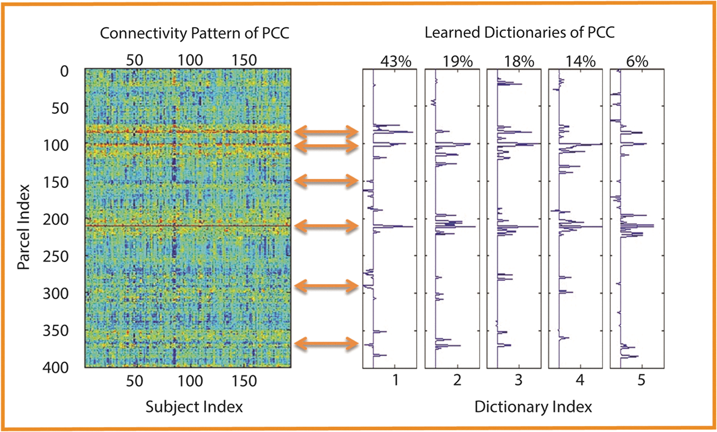
Illustration of the connectomic profile of posterior cingulate cortex or PCC. The left panel shows the whole-brain connectivity patterns of PCC for 193 subjects, and the right panel depicts the corresponding learned dictionary elements. For each of the five elements, the normalized summation of loadings [Eq. (4)] was displayed on the top. The first element was chosen as the connectomic profile of PCC. The orange arrows highlight the correspondence between connectivity pattern and the connectomic profile.

Group RSNs through clustering and their consistency

As well accepted, parcels with similar profiles form a specific spatial pattern or RSN. To identify the RSNs and their corresponding connectomic profiles, we applied the affinity propagation (AP) clustering algorithm (Frey and Dueck, 2007) on the resultant profiles, considered each cluster as a single RSN, and averaged the profiles of involved parcels as that of the RSN. Since AP can automatically determine the optimal number of clusters, we obtained the group consistent RSNs effectively.

Specifically, after the connectomic profiles \documentclass{aastex}\usepackage{amsbsy}\usepackage{amsfonts}\usepackage{amssymb}\usepackage{bm}\usepackage{mathrsfs}\usepackage{pifont}\usepackage{stmaryrd}\usepackage{textcomp}\usepackage{portland, xspace}\usepackage{amsmath, amsxtra}\pagestyle{empty}\DeclareMathSizes{10}{9}{7}{6}\begin{document}$$\textbf{\textit{F}} = \{ \,\textbf{\textit{f}}_1 , \textbf{\textit{f}}_2 , \cdots , \textbf{\textit{f}}_K \} $$ \end{document} were generated for all parcels \documentclass{aastex}\usepackage{amsbsy}\usepackage{amsfonts}\usepackage{amssymb}\usepackage{bm}\usepackage{mathrsfs}\usepackage{pifont}\usepackage{stmaryrd}\usepackage{textcomp}\usepackage{portland, xspace}\usepackage{amsmath, amsxtra}\pagestyle{empty}\DeclareMathSizes{10}{9}{7}{6}\begin{document}$$\textbf{\textit{P}} = \{ p_1 , p_2 , \cdots , p_K \} $$ \end{document} , a similarity matrix was constructed for the AP algorithm (Frey and Dueck, 2007) as follows: \documentclass{aastex}\usepackage{amsbsy}\usepackage{amsfonts}\usepackage{amssymb}\usepackage{bm}\usepackage{mathrsfs}\usepackage{pifont}\usepackage{stmaryrd}\usepackage{textcomp}\usepackage{portland, xspace}\usepackage{amsmath, amsxtra}\pagestyle{empty}\DeclareMathSizes{10}{9}{7}{6}\begin{document} \begin{align*}\textbf{\textit{S}} = \{s_{ij} \,\mid\, s_{ij} = \begin{cases} Corr (\, \textbf{\textit{f}}_i , \textbf{\textit{f}}_j ) \qquad i \ne j \\ \qquad \qquad \qquad \qquad \quad i , j \in [ 1 , K ]\} \ \\ \mu \qquad \qquad \qquad\quad i = j\end{cases} \tag{6}\end{align*} \end{document}

The parameter μ was set as the mean similarity as suggested by (Frey and Dueck, 2007): \documentclass{aastex}\usepackage{amsbsy}\usepackage{amsfonts}\usepackage{amssymb}\usepackage{bm}\usepackage{mathrsfs}\usepackage{pifont}\usepackage{stmaryrd}\usepackage{textcomp}\usepackage{portland, xspace}\usepackage{amsmath, amsxtra}\pagestyle{empty}\DeclareMathSizes{10}{9}{7}{6}\begin{document} \begin{align*}\mu = \frac { 1 } { K ( K - 1 ) } \mathop \sum_i \mathop \sum_j s_ { ij } \ \, for \ i , j \in [ 1 , K ] \ and \ i \ne \,j \tag { 7 } \end{align*} \end{document}

Under definitions in Equations (6) and (7), the outcome of AP algorithm is a set of clusters, \documentclass{aastex}\usepackage{amsbsy}\usepackage{amsfonts}\usepackage{amssymb}\usepackage{bm}\usepackage{mathrsfs}\usepackage{pifont}\usepackage{stmaryrd}\usepackage{textcomp}\usepackage{portland, xspace}\usepackage{amsmath, amsxtra}\pagestyle{empty}\DeclareMathSizes{10}{9}{7}{6}\begin{document}$$\Theta = \{ r_1 , r_2 , \cdots , r_w \} $$ \end{document} , where W is the number of clusters or RSNs automatically determined by the data. The RSN profile rf_l for an RSN \documentclass{aastex}\usepackage{amsbsy}\usepackage{amsfonts}\usepackage{amssymb}\usepackage{bm}\usepackage{mathrsfs}\usepackage{pifont}\usepackage{stmaryrd}\usepackage{textcomp}\usepackage{portland, xspace}\usepackage{amsmath, amsxtra}\pagestyle{empty}\DeclareMathSizes{10}{9}{7}{6}\begin{document}$$r_{\it1} ( l \in [ 1 , W ] )$$ \end{document} , is defined as the mean profiles of involved parcels for current RSN: \documentclass{aastex}\usepackage{amsbsy}\usepackage{amsfonts}\usepackage{amssymb}\usepackage{bm}\usepackage{mathrsfs}\usepackage{pifont}\usepackage{stmaryrd}\usepackage{textcomp}\usepackage{portland, xspace}\usepackage{amsmath, amsxtra}\pagestyle{empty}\DeclareMathSizes{10}{9}{7}{6}\begin{document} \begin{align*}\textbf{\textit{rf}} _l = \frac {1} {\mid r_l \mid} \mathop\sum_{t = 1} \textbf{\textit{f}}_{l , t} , t \in [ 1 , \mid r_l \mid ] \tag{8} \end{align*} \end{document}

where |r_l | is the number of parcels for current RSN r_l . Figure 2 illustrates the profile of the DMN.

FIG. 2.

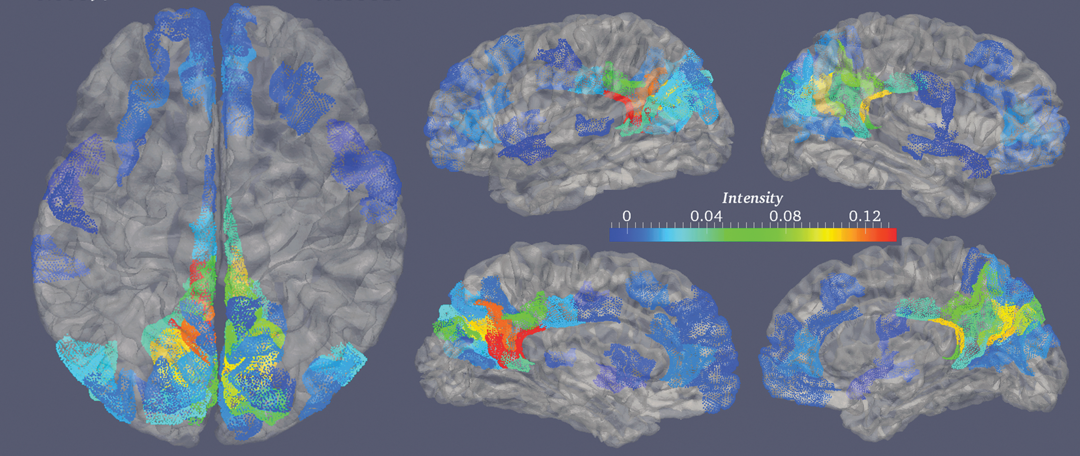
Illustration of the connectomic profile for default mode network (DMN). The left column is the dorsal view. The middle column shows the lateral (top) and medial (bottom) views of the left hemisphere. The right column provides the lateral (top) and medial (bottom) views of the right hemisphere. The color bar displays the intensity of DMN's profile, which indicates how much a region is involved in DMN.

The consistency of the group RSNs was examined on three independent datasets, D1, D2, and D3 in Table 1, through group clustering of the AP algorithm (Frey and Dueck, 2007). A RSN is considered to be consistent only if it is shared by all subjects in the three datasets (n=532). This criterion is stricter than those in previous reports on RSN consistency (Damoiseaux et al., 2006; Moussa et al., 2012; Zuo et al., 2010). Specifically, three sets of group RSNs were generated from D1 to D3. Subsequently, each RSN was considered as a data point and the similarity between any two points was calculated as according to Equation (6). The resultant clusters that have members from all datasets were considered common and consistent.

Individual RSN/ROI generation through optimization

To identify ROIs for an individual, we first defined a set of ROIs according to the profile intensity for any derived group RSN in the previous section, as shown in Figure 3. Let T be one of these ROIs, its individual counterpart \documentclass{aastex}\usepackage{amsbsy}\usepackage{amsfonts}\usepackage{amssymb}\usepackage{bm}\usepackage{mathrsfs}\usepackage{pifont}\usepackage{stmaryrd}\usepackage{textcomp}\usepackage{portland, xspace}\usepackage{amsmath, amsxtra}\pagestyle{empty}\DeclareMathSizes{10}{9}{7}{6}\begin{document}$$\hat{C}$$ \end{document} is the parcel that minimizes the following energy function: \documentclass{aastex}\usepackage{amsbsy}\usepackage{amsfonts}\usepackage{amssymb}\usepackage{bm}\usepackage{mathrsfs}\usepackage{pifont}\usepackage{stmaryrd}\usepackage{textcomp}\usepackage{portland, xspace}\usepackage{amsmath, amsxtra}\pagestyle{empty}\DeclareMathSizes{10}{9}{7}{6}\begin{document} \begin{align*}\hat{C} = \arg\displaylimits_{C{ \in} N_{T}} \min \{ \omega E_{{ \rm int}} + ( 1 - \omega ) E_{ext} \} \tag{9}\end{align*} \end{document}

FIG. 3.

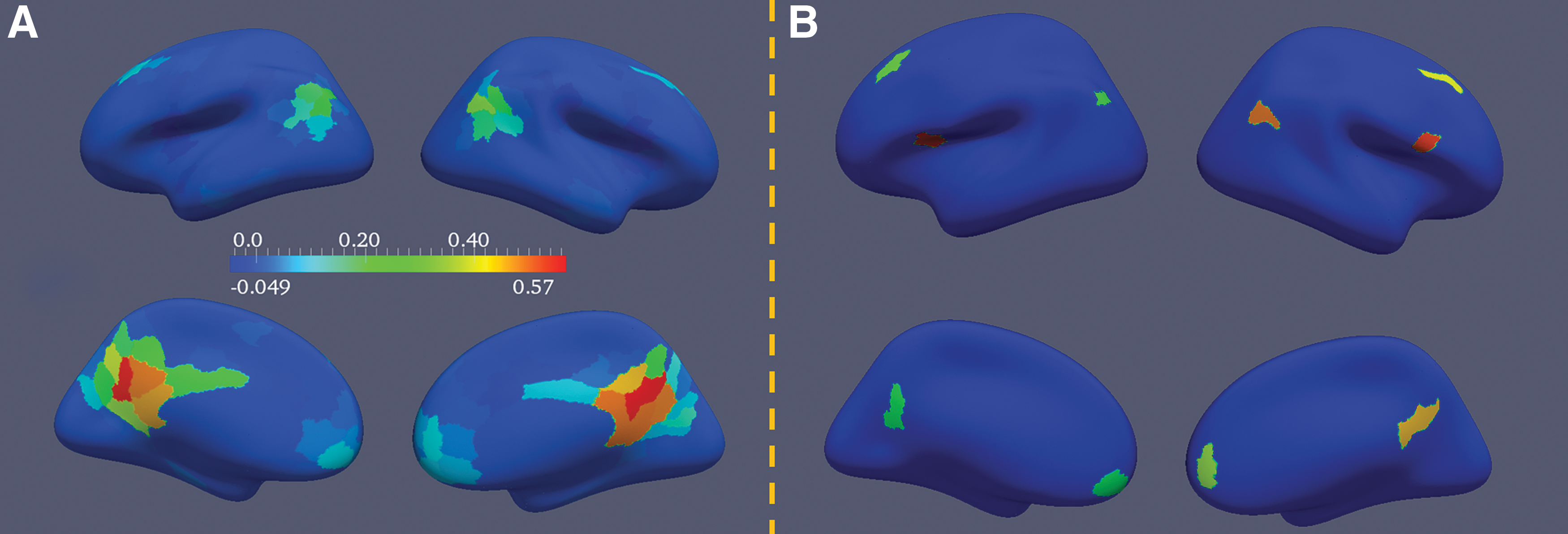
Illustration of region of interest (ROI) section for the DMN. (A) The profile of the DMN in Figure 2 mapped onto an inflated cortical surface. (B) The selected ROIs for the DMN.

where σ is the standard deviation of T's distribution on the template space, estimated by registering T's counterparts for all subjects to the template space, and d is the geodesic distance between the centers of two parcels T_i and the candidate C: \documentclass{aastex}\usepackage{amsbsy}\usepackage{amsfonts}\usepackage{amssymb}\usepackage{bm}\usepackage{mathrsfs}\usepackage{pifont}\usepackage{stmaryrd}\usepackage{textcomp}\usepackage{portland, xspace}\usepackage{amsmath, amsxtra}\pagestyle{empty}\DeclareMathSizes{10}{9}{7}{6}\begin{document} \begin{align*}d = \parallel S_{T_{i}} - S_C \parallel_G \tag{11}\end{align*} \end{document}

In Equation (11), S _[•] is the spherical coordinate of a parcel on the template, and ||•||_G is the geodesic distance between two spherical coordinates. The external energy is defined as the distance between the connectomic profile f _T of T and the connectivity pattern x_C of C: \documentclass{aastex}\usepackage{amsbsy}\usepackage{amsfonts}\usepackage{amssymb}\usepackage{bm}\usepackage{mathrsfs}\usepackage{pifont}\usepackage{stmaryrd}\usepackage{textcomp}\usepackage{portland, xspace}\usepackage{amsmath, amsxtra}\pagestyle{empty}\DeclareMathSizes{10}{9}{7}{6}\begin{document} \begin{align*}E_{ext} = 1 - Corr ( \textbf{\textit{x}}_C , \textbf{\textit{f}}_T ) \tag{12}\end{align*} \end{document}

Results

Cortical parcellation

To evaluate the overall parcellation performance of different methods, a metric, η, was defined to reflect the BOLD signal homogeneity of all parcels of the cortex: \documentclass{aastex}\usepackage{amsbsy}\usepackage{amsfonts}\usepackage{amssymb}\usepackage{bm}\usepackage{mathrsfs}\usepackage{pifont}\usepackage{stmaryrd}\usepackage{textcomp}\usepackage{portland, xspace}\usepackage{amsmath, amsxtra}\pagestyle{empty}\DeclareMathSizes{10}{9}{7}{6}\begin{document}$$\eta = \bar{r} / \sigma_r$$ \end{document} , where \documentclass{aastex}\usepackage{amsbsy}\usepackage{amsfonts}\usepackage{amssymb}\usepackage{bm}\usepackage{mathrsfs}\usepackage{pifont}\usepackage{stmaryrd}\usepackage{textcomp}\usepackage{portland, xspace}\usepackage{amsmath, amsxtra}\pagestyle{empty}\DeclareMathSizes{10}{9}{7}{6}\begin{document}$$\textbf{\textit{r}} = \{ r_1 , r_2 , r_3 , \ldots r_K \} $$ \end{document} are the explained variance fraction of the first principal vectors of BOLD signals for the K parcels \documentclass{aastex}\usepackage{amsbsy}\usepackage{amsfonts}\usepackage{amssymb}\usepackage{bm}\usepackage{mathrsfs}\usepackage{pifont}\usepackage{stmaryrd}\usepackage{textcomp}\usepackage{portland, xspace}\usepackage{amsmath, amsxtra}\pagestyle{empty}\DeclareMathSizes{10}{9}{7}{6}\begin{document}$$\textbf{\textit{P}} = \{ p_1 , p_2 , \cdots , p_K \} $$ \end{document} , \documentclass{aastex}\usepackage{amsbsy}\usepackage{amsfonts}\usepackage{amssymb}\usepackage{bm}\usepackage{mathrsfs}\usepackage{pifont}\usepackage{stmaryrd}\usepackage{textcomp}\usepackage{portland, xspace}\usepackage{amsmath, amsxtra}\pagestyle{empty}\DeclareMathSizes{10}{9}{7}{6}\begin{document}$$\bar{r}$$ \end{document} and σ_r are the mean value and standard deviation of these ratios, respectively. Intuitively, the higher the value of r, the more homogeneous the BOLD signals; meanwhile, a lower σ_r indicates a more consistent parcellation. Together, a higher η corresponds to a parcellation that generates more homogeneous parcels consistently for the whole cortex. Using this metric, we evaluate the cortical parcellation results of our method. A comparison parcellation was performed on dataset D1 (n=193). It was based on surface registration (Fischl et al., 1999) of a parceled cortex with the same parcel sizes as our results, but with random edge weights E which were sampled from the standard uniform distribution, that is, E ∼ U(0,1).

Figure 4A–C depicts the cortical parcellation for a random subject in three different views. The cortical vertices that belong to one parcel are rendered by the same color. Neighboring parcels are rendered with distinct colors, and parcels with the same color indicate nothing other than that they are not neighbors. As can be seen in these panels, our method can generate smooth and continuous parcels for the cortex, indicating that the geodesic spatial regularization works as expected. Additionally, the resultant parcels are balanced in terms of parcel size, with a mean and standard deviation of 430.5±69.0 mm². The largest parcel has a surface area about twice that of the smallest parcel.

FIG. 4.

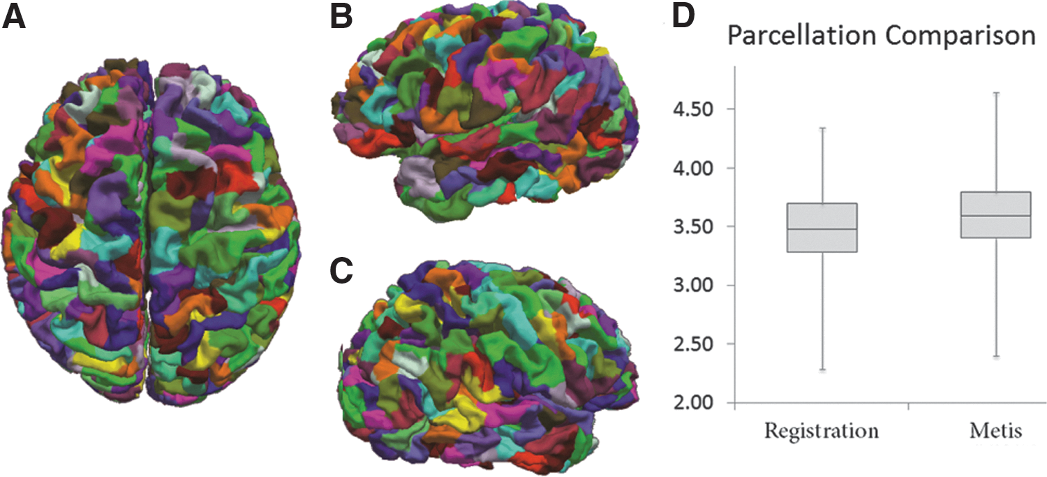
Cortical parcellation by the framework. (A–C) Are illustrations of the cortical parcellation. (A) Dorsal view. (B, C) Lateral views. The parcels are colored in a way that neighboring parcels have different colors, and parcels with the same color mean nothing, except that they are not neighbors. (D) Shows the box-and-whisker diagram of η values for both registration based parcellation and the present method.

Figure 4D depicts the comparison of performances of the two parcellation methods examined in this work. Compared with surface registration-based parcellation (Fischl et al., 1999), our result has significantly improved the parcel homogeneity (p-value <1.0×10⁻¹⁰), as revealed by the increase of η. This indicates that the present parcellation led to improved homogeneous parcels for subsequent analysis.

Consistent group profiles and RSNs

In this section, we describe validation of the configuration of dictionary learning for a parcel's connectomic profile and present the group RSNs that are consistent across datasets D1, D2, and D3. While learning a parcel's connectomic profile, different dictionary elements correspond to different connectivity patterns and were designed to represent the connectomic variation due to anatomical variability in a group. In this study, the number of dictionary elements was set to five for each parcel. The dominant dictionary element corresponding to the maximum summation of loadings is considered as the connectomic profile for this parcel whereas the one corresponding to the minimum summation of loadings is the trivial element [see Eqs. (4) and ((5) for definitions]. The fraction of people sharing trivial elements would be very low if there are enough dictionary elements to capture the variability of connectivity patterns within the studied groups.

Figure 5A and B shows the percentage of subjects in dataset D1 that share the same dominant dictionary element and the trivial element, respectively. The mean fraction of subjects sharing dominant dictionary elements is 40.80%, averaged on 400 parcels, whereas those sharing trivial dictionary elements is only 3.43%. This indicates that the dominant dictionary element captures the common and consistent connectivity pattern of a parcel for a group, and that five dictionary elements in Equations (2) and (3) is sufficient to capture the majority of a parcel's connectional variability for the studied group.

FIG. 5.

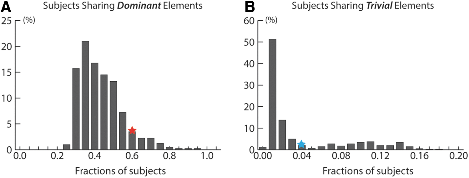
Histograms for fractions of subjects sharing same dictionary elements. (A, B) Are the histograms of fractions of subjects that share dominant and trivial dictionary elements, respectively. For both figures, the horizontal axis refers to the fraction of subjects sharing the same dictionary elements, for example, 0.8 at the X-axis in (A) means 80% of subjects have the same dominant connectomic pattern, whereas the vertical axis indicates how many parcels out of 400 have the same fraction. For instance, the red star in (A) indicates that there are ∼4% parcels, where 60% subjects share the same dominant connectomic patterns, whereas the blue star in (B) indicates there are ∼2% parcels where 4% subjects have the same trivial connectomic patterns. (A) Small fraction value (averaged at 3.43%) in (B) indicates five dictionary elements in the present model is sufficient.

We performed a consistency study based on datasets D1–D3 (n=532 in total) and summarized the result in panel D of Figure 6. Dataset D1 generated 46 group RSNs, whereas datasets D2 and D3 generated 45 and 44, respectively. Although the numbers of resultant RSNs are very close, these RSNs are not identical. The majority (∼60%, 27 RSNs in total) of these resultant RSNs is consistent across different datasets and a significant fraction (∼40%) of them show variations that might be caused by the demographic differences or brain dynamics. The number of consistent RSNs is similar to that reported in another study (Naveau et al., 2012), which identify 28 consistent RSNs based on data from 310 subjects. In the rest of this article, we focus on the 27 consistent RSNs across groups.

FIG. 6.

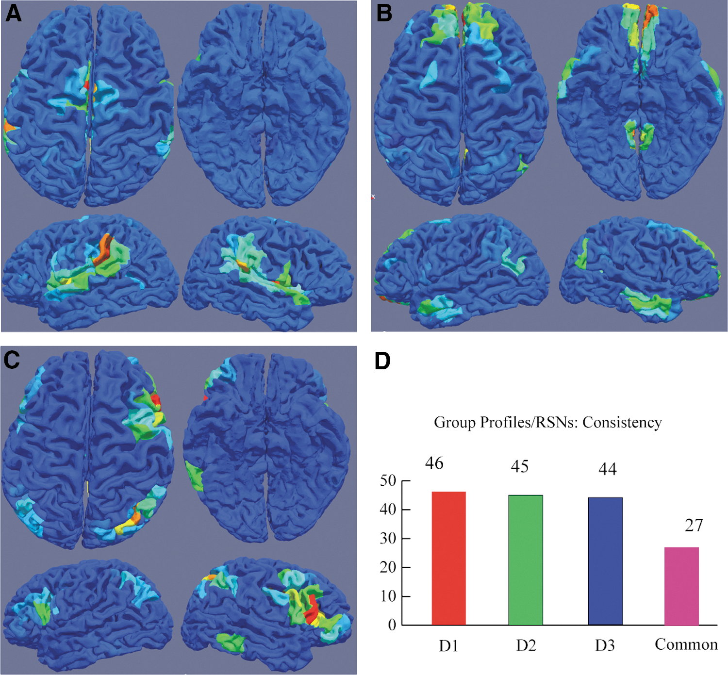
Common group resultant functional networks (RSNs) and their profiles. (A–C) Illustrate profiles of three group RSNs, that is, temporal–parietal junction, DMN, and ventral attention network, respectively. For each RSN profile, there are four subfigures that show different views, that is, dorsal, ventral, and bilateral. (D) Summarizes the common RSNs across three datasets D1, D2, and D3.

Figure 6A–C illustrates the group profiles of three consistent RSNs. Each group RSN's profile has four different views. Panel A shows the connections of the temporal parietal junction with insular cortex, mid-cingulate, as well as dorsal lateral prefrontal cortex. Panel B presents the DMN, and panel C depicts the ventral attention network. The spatial patterns of these group RSNs are similar to those reported using ICA analysis (Damoiseaux et al., 2006; Zuo et al., 2010). Due to space limitation, only three group RSNs and their profiles are described in the manuscript, but all 27 consistent RSNs and profiles can be found at http://bitc.bme.emory.edu/∼kli/connectomicProfile.

Individual ROIs of consistent RSNs

To ascertain whether Equation (9) improves ROIs' functional correspondence, 211 ROIs of the 27 consistent RSNs were generated for each individual through the present method and surface-based registration (Fischl et al., 1999), respectively. For the latter, the 211 ROIs in the template space were mapped to individuals through surface-based registration (Fischl et al., 1999). For each generated ROI, its similarity to its corresponding RSN is measured by the Pearson correlation coefficient between its spatial connectivity pattern and the RSN's connectomic profile. For both methods, similarities of ROIs within the same RSN were averaged. A paired t-test assuming equal sample variance was then conducted for method difference. The same test was performed on datasets D1 and D2, respectively, and the results are summarized in Figure 7. As can be seen, our method performs significantly better (*p<1.0×10⁻⁶, corrected using false discovery rate (FDR) [Storey, 2002]) for 24 out of 27 RSNs, and the result is consistent across datasets D1 and D2, indicating that the present algorithm is robust and superior over the registration method (Fischl et al., 1999) in localizing functional regions. Another interesting observation is that we do not see significant improvement in performance for RSNs 7, 13, and 23 for both datasets. The reason for the lack of improvement might be that the ROIS of these RSNs are dorsal and ventral visual networks, and are too close for the anatomical constraint to be beneficial. As such, the resultant ROIs through the present framework are comparable to those through the registration method (Fischl et al., 1999).

FIG. 7.

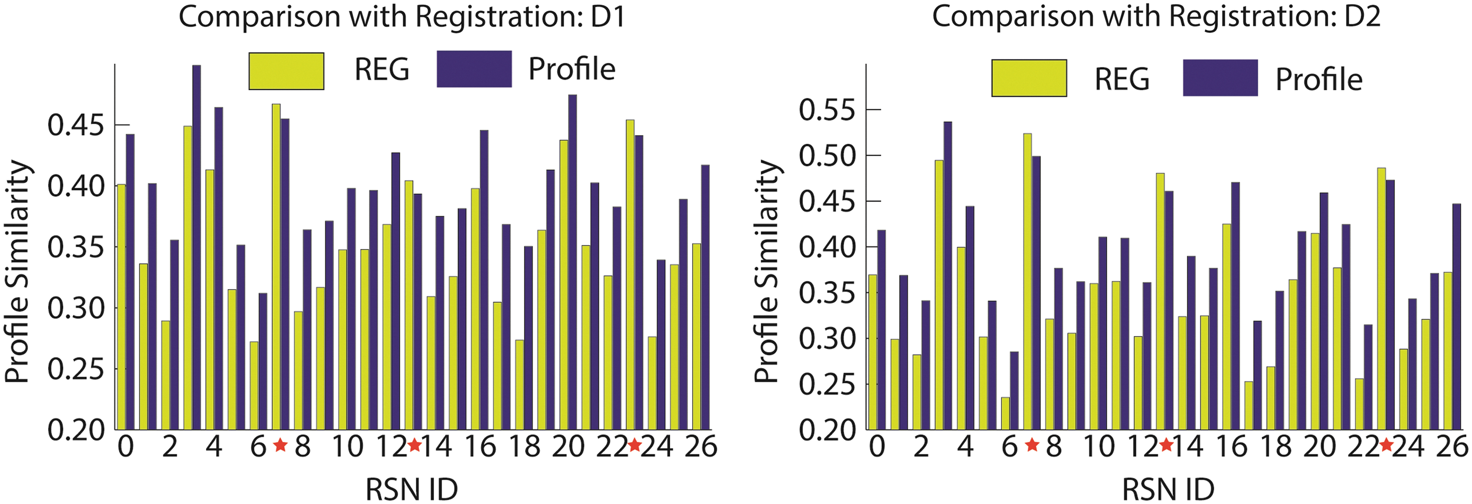
Comparison of individual RSNs with surface registration. The two figures compare the individual ROIs' functional correspondence between surface-based registration (REG) and our framework (Profile) for datasets D1 and D2. Horizontal axis denotes the 27 consistent RSNs, and vertical axis is the correlation coefficient of a ROI's connectivity pattern with the connectomic profile of corresponding RSN. All RSNs except those with red stars have significant improvements.

Test–retest and reproducibility study

To test the reproducibility and reliability of our framework, we applied it to dataset D4, which contains three sessions of rsfMRI scans for a cohort of normal subjects (Zuo et al., 2010). The time interval between sessions 1 and 2 is ∼11 months, whereas that between sessions 2 and 3 is ∼45 min (Zuo et al., 2010). For each session, the 211 ROIs of the 27 consistent RSNs were determined for each individual through our method, and Pearson correlation coefficients between the connectivity patterns of these ROIs and the connectomic profiles of their corresponding RSNs were calculated and averaged within networks. The averaged correlation coefficients of the same RSN from different sessions were tested using a paired t-test assuming equal variances for differences. The resultant p-values were corrected using FDR (Benjamini and Hochberg, 1995). If the present method can robustly and accurately identify individual ROIs for common RSNs, the correlation coefficients for the same subject from repeated sessions should not be significantly changed. For simplicity, the statistical test between session 1 and session 2 is referred to as p12, and p13 and p23 are similarly defined.

Figure 8 shows the averaged correlation coefficients for the 27 common RSNs of the three sessions, and the statistical tests of these coefficients between the three sessions were summarized in Figure 9. As can be seen in Figures 8 and 9, there is no significant difference for any of the tests, indicating that the spatial patterns of the individualized ROIs generated by our method do not change significantly across either a short interval or a long interval. This further demonstrates that the 27 group RSNs are common across individuals and that our method can robustly generate consistent ROIs of these group RSNs for individuals across sessions. Despite the overall consistency of the group profiles across sessions, it is worth noting that p23 exhibits more consistency than the other comparisons, as revealed by the much larger corrected p-values of p23 than those of p12 and p13. The result is expected and reasonable considering the time interval between sessions 2 and 3 (about 45 min) is much shorter than that between sessions 1 and 2/3 (about 11 months). This also indicates that the functional regions may undergo longitudinal changes in terms of their connectomic profiles after a considerable time.

FIG. 8.

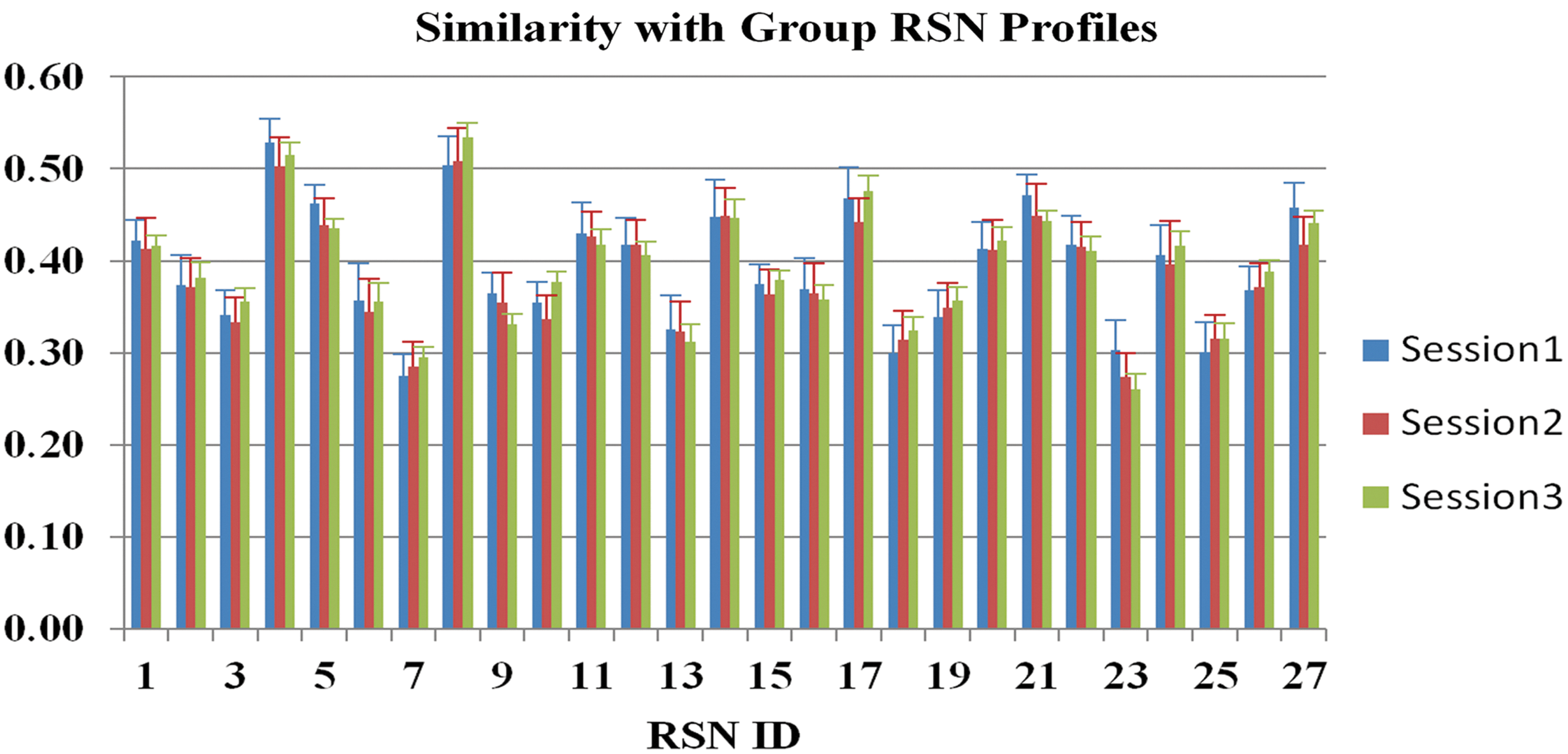
Similarity of individual RSNs with the group connectomic profiles. Horizontal axis is RSN ID, and vertical axis is the similarity of individual RSNs with the connectomic profiles. Each similarity was averaged across 23 subjects, and the error bar shows the standard deviation. For each RSN, similarities from three sessions of the group are depicted.

FIG. 9.

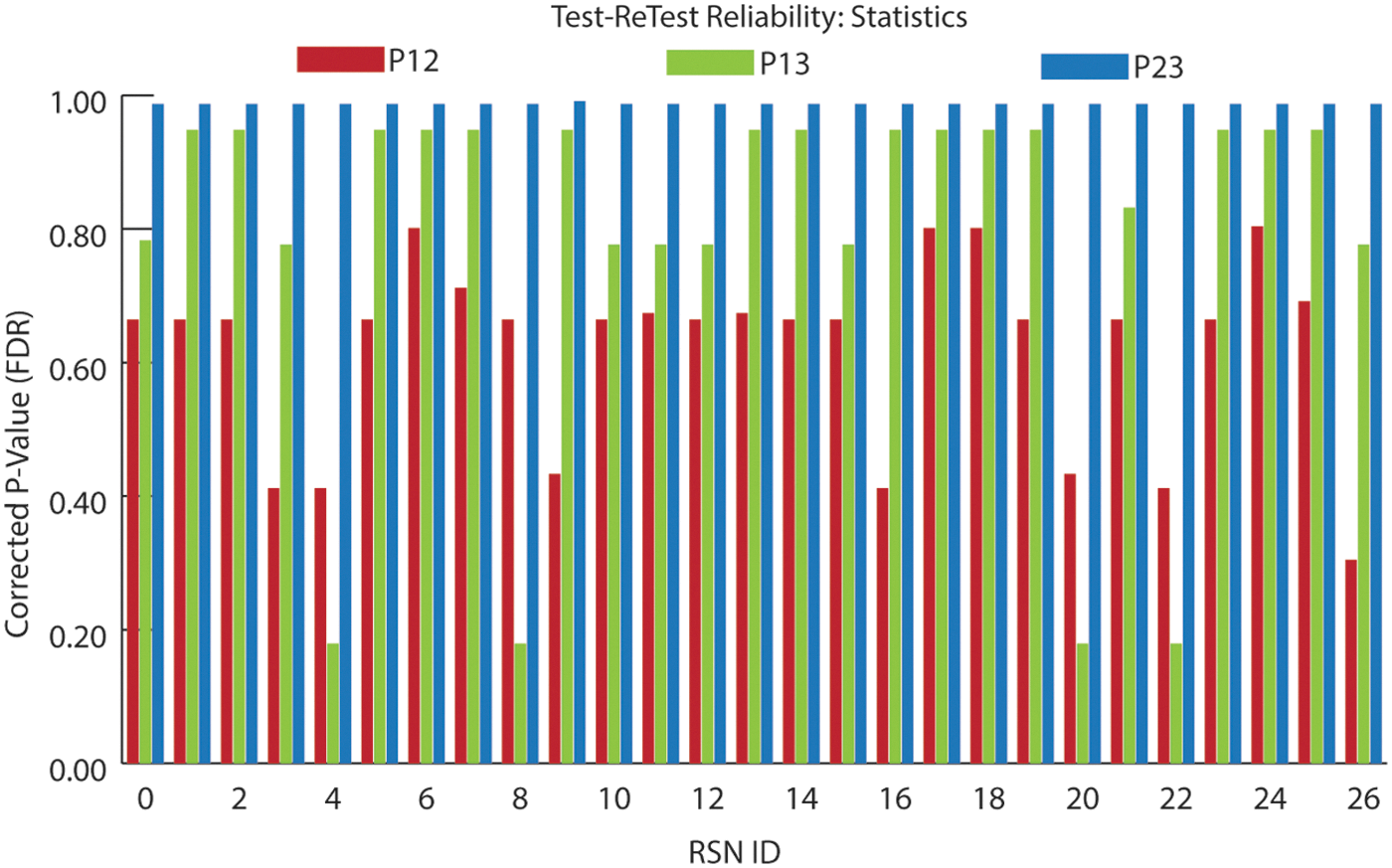
Test and retest of the individual ROIs/RSNs through our framework. Horizontal axis is RSN ID, and vertical axis is the corrected p-value using false discovery rate (FDR). P12 compares the connectivity patterns of individual ROIs from sessions 1 and 2 with the group connectomic profile of corresponding RSN. P13 compares sessions 1 and 3, and P23 is for sessions 2 and 3.

Discussion and Conclusion

In this article, we present an algorithmic framework for identifying functional ROIs and RSNs for individuals. Instead of using only anatomical-based registration, we employ both anatomical and group connectomic profile constraints to localize the involved functional ROIs of RSNs for individuals. The group connectomic profiles were generated through dictionary learning based on large rsfMRI datasets, and their consistency was examined on three datasets (n=532), generating 27 common RSNs. These large-scale experiments demonstrate that our framework has superior performance in terms of functional correspondence compared with anatomical registration. A test–retest study also reveals that the framework is robust and consistent across both short- and long-interval sessions.

Different from recent advances of cortical parcellation through rsfMRI (Craddock et al., 2012; Shen et al., 2010, 2013; van den Heuvel et al., 2008a), the role of cortical parcellation in the present work is not to parcellate the cortex into parcels that have one-by-one correspondence across subjects, but to provide a set of functionally homogeneous substrates for subsequent analysis. Since anatomical registration does not provide a perfect voxel-to-voxel correspondence across subjects due to huge anatomical variability (Ng et al., 2012; Roland et al., 1997; Zhu et al., 2013), estimation of connectomic profile of a functional ROI at the voxel level using multi-subject datasets would be inaccurate and ineffective (Blumensath et al., 2013). Thus, subdividing the neocortex into functionally homogeneous regions can relax the voxel-by-voxel correspondence problem to a parcel-by-parcel one and lays the foundation for subsequent analysis that accounts for individual anatomical variability. It is also beneficial in terms of reducing data dimension and enhancing signal-to-noise ratio. In essence, parcellation in the present work provides functionally homogeneous substrates for subsequent analysis at a more macro scale than the voxel-to-vertex level.

An important yet open issue in the brain imaging community is the choice of the number of parcels, K, during the parcellation of the cortex. The optimal K in our opinion may be dependent on data acquisition and applications. For instance, there are multiple successful studies (Achard et al., 2006; Liu et al., 2008; Salvador et al., 2005) using existing structural atlas, for example, automated anatomical labeling (Tzourio-Mazoyer et al., 2002), which parcel the whole brain into 90–116 regions. Recently, the cortex was further parceled for fine-granularity regions based on FC patterns (Beckmann et al., 2009; Kahn et al., 2008; Margulies et al., 2007) The purpose of cortical parcellation in our study, however, is not to acquire the ultimate functional ROIs, but to provide substrates that may have better correspondence across subjects than voxel/vertex-wise registration and to improve the signal-to-noise ratio for subsequent analysis. Such a purpose is different from those of fine-granularity cortical parcellation studies (Beckmann et al., 2009; Kahn et al., 2008; Margulies et al., 2007) and from those of cortical boundary studies based on abrupt FC changes (Cohen et al., 2008; Wig et al., 2014). In present study, we preferred a large number of parcels (K=400, in accordance with recent cortical segregation studies) (Kaas, 2008; Van Essen et al., 2012) to make sure that the resultant regions are functionally homogeneous.

Dictionary learning has two roles in the present study. First, anatomical variability still exists after we convert the voxel-to-voxel correspondence problem to a parcel-to-parcel one with the cortical parcellation, although it is mitigated through registration and parcellation. Therefore, there is a need to model the variable connectivity pattern induced by anatomical variability when extracting the group-wise connectomic profiles for a parcel. This variability in connectivity pattern can be embedded as dictionary elements in dictionary learning. Second, since the BOLD signals are noisy, it is common for a functional region to appear to be connected to all other functional regions in the connectivity pattern. Thus, we need to remove false positive connections due to noise; this could be achieved by imposing sparsity constraints in each dictionary element.

Two types of sparsity constraints were imposed in our method to learn the group-wise consistent connectomic profiles, as shown in Equations (2) and (3). The first is on the loading α_i that corresponds to the connectivity pattern x_i . This sparsity selects a limited number of dictionary elements (<λ) to represent current connectivity pattern x_i . In this study, λ is two, indicating that only one dictionary element can be selected to represent a certain connectivity pattern x_i . Combined with Equation (4), the resultant connectomic profile removes the variability of connectivity pattern induced by anatomical variability. The second type of sparsity is on the dictionary element d_j in Equation (3). Each dictionary element d_j is both smooth in the solution space, as constrained by the second-order matrix norm, and sparse, as constrained by the first-order matrix norm. Together with the first sparsity constraint, it helps eliminate the false positives in the connectivity pattern resulting from noise and extracts the group-wise consistent connectomic profile by excluding connectivity patterns exhibiting significant individual variability.

The consistency of RSNs has been reported in literature (Damoiseaux et al., 2006; Moussa et al., 2012; Zuo et al., 2010). The number of consistent RSNs reported, however, is not consistent. For example, Damoiseaux and colleagues (2006) reported 10 RSNs using two independent datasets, whereas Zuo and colleagues (2010) adopted 20 group RSNs in their study. In addition, Moussa and colleagues (2012) found that even commonly reported RSNs are not consistent across subjects. Our consistency study, based on three large rsfMRI datasets (n=532 in total), identified 27 consistent RSNs, considerably higher than the previous reports. The reason may be that our framework accounts for anatomical variability and false positive connectivity by cortical parcellation and dictionary learning. These two critical steps help reduce the effect of anatomical variability better than registration, reduce false positive connections due to noise, and extract more consistent RSNs that would be otherwise contaminated.

The generation of RSNs/ROIs for individuals was formulated as an energy minimization problem with two types of constraints. An internal energy, E_int , imposes anatomical constraint so that the corresponding functional regions across subjects have a similar location in the template space, and it only works at the coarse level due to the limited accuracy of spatial registration (Li et al., 2012a; Zhu et al., 2013). An external energy, E_ext , imposes connectomic constraint so that corresponding functional regions across subjects have a similar connectivity pattern. Unlike E_int , E_ext only works at the fine level, since two remote functional ROIs of one RSN could have very similar connectomic profiles. Together, these two energies facilitate the establishment of ROI correspondences across individuals both anatomically and functionally. The model configuration and parameter settings were kept the same with our previous publications (Li et al., 2010, 2012b), since the problems to be solved in these minimization models are essentially the same.

There are some pitfalls that need to be noted in the present work. First, in the reproducibility study, our tests showed there was no significant change in the correlation between the connectivity patterns and the connectomic profiles across sessions. This is an indirect test of the consistency of the spatial patterns, and direct tests need to be studied in the future. Another pitfall is that the RSNs generated through our framework are static. Considering that there are complex dynamics between the ROIs of these RSNs, future work will focus on the dynamics of RSNs with the identified individual ROIs. We believe the individually-tuned accurate ROIs will provide solid substrates for functional analysis.

Footnotes

Acknowledgments

The authors would like to thank the 1000 Functional Connectomes Project for data sharing. This work was supported by the National Institutes of Health (grant number R01-DA033393).

Author Disclosure Statement

No competing financial interests exist.

References

Achard

, Salvador

, Whitcher

, Suckling

, Bullmore

. 2006. A resilient, low-frequency, small-world human brain functional network with highly connected association cortical hubs. J Neurosci, 26:63–72.

Beckmann

, Johansen-Berg

, Rushworth

. 2009. Connectivity-based parcellation of human cingulate cortex and its relation to functional specialization. J Neurosci, 29:1175–1190.

Benjamini

, Hochberg

. 1995. Controlling the false discovery rate—a practical and powerful approach to multiple testing. J R Stat Soc Series B Methodol, 57:289–300.

Bluhm

, Miller

, Lanius

, Osuch

, Boksman

, Neufeld

, Theberge

, Schaefer

, Williamson

. 2007. Spontaneous low-frequency fluctuations in the BOLD signal in schizophrenic patients: anomalies in the default network. Schizophr Bull, 33:1004–1012.

Blumensath

, Jbabdi

, Glasser

, Van Essen

, Ugurbil

, Behrens

, Smith

. 2013. Spatially constrained hierarchical parcellation of the brain with resting-state fMRI. Neuroimage, 76:313–324.

Brookes

, Woolrich

, Luckhoo

, Price

, Hale

, Stephenson

, Barnes

, Smith

, Morris

. 2011. Investigating the electrophysiological basis of resting state networks using magnetoencephalography. Proc Natl Acad Sci U S A, 108:16783–16788.

Calhoun

, Liu

, Adali

. 2009. A review of group ICA for fMRI data and ICA for joint inference of imaging, genetic, and ERP data. Neuroimage, 45:S163–S172.

Chang

, Glover

. 2010. Time-frequency dynamics of resting-state brain connectivity measured with fMRI. Neuroimage, 50:81–98.

Cohen

, Fair

, Dosenbach

, Miezin

, Dierker

, Van Essen

, Schlaggar

, Petersen

. 2008. Defining functional areas in individual human brains using resting functional connectivity MRI. Neuroimage, 41:45–57.

10.

Craddock

, James

, Holtzheimer

3rd , Hu

, Mayberg

. 2012. A whole brain fMRI atlas generated via spatially constrained spectral clustering. Hum Brain Mapp, 33:1914–1928.

11.

Damoiseaux

, Rombouts

, Barkhof

, Scheltens

, Stam

, Smith

, Beckmann

. 2006. Consistent resting-state networks across healthy subjects. Proc Natl Acad Sci U S A, 103:13848–13853.

12.

Dastjerdi

, Foster

, Nasrullah

, Rauschecker

, Dougherty

, Townsend

, Chang

, Greicius

, Menon

, Kennedy

, Parvizi

. 2011. Differential electrophysiological response during rest, self-referential, and non-self-referential tasks in human posteromedial cortex. Proc Natl Acad Sci U S A, 108:3023–3028.

13.

Fischl

, Sereno

, Dale

. 1999. Cortical surface-based analysis. II: inflation, flattening, and a surface-based coordinate system. Neuroimage, 9:195–207.

14.

Frey

, Dueck

. 2007. Clustering by passing messages between data points. Science, 315:972–976.

15.

Greicius

, Krasnow

, Reiss

, Menon

. 2003. Functional connectivity in the resting brain: a network analysis of the default mode hypothesis. Proc Natl Acad Sci U S A, 100:253–258.

16.

Greicius

, Srivastava

, Reiss

, Menon

. 2004. Default-mode network activity distinguishes Alzheimer's disease from healthy aging: evidence from functional MRI. Proc Natl Acad Sci U S A, 101:4637–4642.

17.

Gusnard

, Raichle

. 2001. Searching for a baseline: functional imaging and the resting human brain. Nat Rev Neurosci, 2:685–694.

18.

Jenkinson

, Bannister

, Brady

, Smith

. 2002. Improved optimization for the robust and accurate linear registration and motion correction of brain images. Neuroimage, 17:825–841.

19.

Kaas

. 2008. The evolution of the complex sensory and motor systems of the human brain. Brain Res Bull, 75:384–390.

20.

Kahn

, Andrews-Hanna

, Vincent

, Snyder

, Buckner

. 2008. Distinct cortical anatomy linked to subregions of the medial temporal lobe revealed by intrinsic functional connectivity. J Neurophysiol, 100:129–139.

21.

Karypis

, Kumar

. 1998. A fast and high quality multilevel scheme for partitioning irregular graphs. SIAM J Sci Comput, 20:359–392.

22.

Kennedy

, Redcay

, Courchesne

. 2006. Failing to deactivate: resting functional abnormalities in autism. Proc Natl Acad Sci U S A, 103:8275–8280.

23.

, Guo

, Faraco

, Zhu

, Chen

, Yuan

, Lv

, Deng

, Jiang

, Zhang

, Hu

, Zhang

, Miller

, Liu

. 2012a. Visual analytics of brain networks. Neuroimage, 61:82–97.

24.

, Guo

, Faraco

, Zhu

, Deng

, Zhang

, Jiang

, Zhang

, Chen

, Hu

. 2010. Individualized ROI optimization via maximization of groupwise consistency of structural and functional profiles. Neural Inf Process Syst, 23:1369–1377.

25.

, Guo

, Zhu

, Hu

, Han

, Liu

. 2012b. Individual functional ROI optimization via maximization of group-wise consistency of structural and functional profiles. Neuroinformatics, 10:225–242.

26.

Liu

. 2011. A few thoughts on brain ROIs. Brain Imaging Behav, 5:189–202.

27.

Liu

, Liang

, Zhou

, He

, Hao

, Song

, Yu

, Liu

, Jiang

. 2008. Disrupted small-world networks in schizophrenia. Brain, 131:945–961.

28.

Lund

, Madsen

, Sidaros

, Luo

W-L

, Nichols

. 2006. Non-white noise in fMRI: does modelling have an impact?. Neuroimage, 29:54–66.

29.

Mairal

, Bach

, Ponce

, Sapiro

. 2010. Online learning for matrix factorization and sparse coding. J Mach Learn Res, 11:19–60.

30.

Margulies

, Kelly

, Uddin

, Biswal

, Castellanos

, Milham

. 2007. Mapping the functional connectivity of anterior cingulate cortex. Neuroimage, 37:579–588.

31.

Moussa

, Steen

, Laurienti

, Hayasaka

. 2012. Consistency of network modules in resting-state FMRI connectome data. PLoS One, 7:e44428.

32.

Naveau

, Doucet

, Delcroix

, Petit

, Zago

, Crivello

, Jobard

, Mellet

, Tzourio-Mazoyer

, Mazoyer

, Joliot

. 2012. A novel group ICA approach based on multi-scale individual component clustering. Application to a large sample of fMRI data. Neuroinformatics, 10:269–285.

33.

, Hamarneh

, Abugharbieh

. 2012. Modeling brain activation in fMRI using group MRF. IEEE Trans Med Imaging, 31:1113–1123.

34.

Roland

, Geyer

, Amunts

, Schormann

, Schleicher

, Malikovic

, Zilles

. 1997. Cytoarchitectural maps of the human brain in standard anatomical space. Hum Brain Mapp, 5:222–227.

35.

Salvador

, Suckling

, Coleman

, Pickard

, Menon

, Bullmore

. 2005. Neurophysiological architecture of functional magnetic resonance images of human brain. Cereb Cortex, 15:1332–1342.

36.

Shen

, Papademetris

, Constable

. 2010. Graph-theory based parcellation of functional subunits in the brain from resting-state fMRI data. Neuroimage, 50:1027–1035.

37.

Shen

, Tokoglu

, Papademetris

, Constable

. 2013. Groupwise whole-brain parcellation from resting-state fMRI data for network node identification. Neuroimage, 82:403–415.

38.

Smith

, Miller

, Salimi-Khorshidi

, Webster

, Beckmann

, Nichols

, Ramsey

, Woolrich

. 2011. Network modelling methods for FMRI. Neuroimage, 54:875–891.

39.

Storey

. 2002. A direct approach to false discovery rates. J R Stat Soc Series B Stat Methodol, 64:479–498.

40.

Thirion

, Flandin

, Pinel

, Roche

, Ciuciu

, Poline

. 2006. Dealing with the shortcomings of spatial normalization: multi-subject parcellation of fMRI datasets. Hum Brain Mapp, 27:678–693.

41.

Tzourio-Mazoyer

, Landeau

, Papathanassiou

, Crivello

, Etard

, Delcroix

, Mazoyer

, Joliot

. 2002. Automated anatomical labeling of activations in SPM using a macroscopic anatomical parcellation of the MNI MRI single-subject brain. Neuroimage, 15:273–289.

42.

van den Heuvel

, Mandl

, Hulshoff Pol

. 2008a. Normalized cut group clustering of resting-state FMRI data. PLoS One, 3:e2001.

43.

van den Heuvel

, Stam

, Boersma

, Hulshoff Pol

. 2008b. Small-world and scale-free organization of voxel-based resting-state functional connectivity in the human brain. Neuroimage, 43:528–539.

44.

Van Essen

, Glasser

, Dierker

, Harwell

, Coalson

. 2012. Parcellations and hemispheric asymmetries of human cerebral cortex analyzed on surface-based atlases. Cereb Cortex, 22:2241–2262.

45.

Varoquaux

, Craddock

. 2013. Learning and comparing functional connectomes across subjects. Neuroimage, 80:405–415.

46.

Varoquaux

, Gramfort

, Pedregosa

, Michel

, Thirion

. 2011. Multi-subject dictionary learning to segment an atlas of brain spontaneous activity. Inf Process Med Imaging, 22:562–573.

47.

Wig

, Laumann

, Cohen

, Power

, Nelson

, Glasser

, Miezin

, Snyder

, Schlaggar

, Petersen

. 2014. Parcellating an individual subject's cortical and subcortical brain structures using snowball sampling of resting-state correlations. Cereb Cortex, 24:2036–2054.

48.

Zhu

, Li

, Guo

, Jiang

, Zhang

, Chen

, Deng

, Faraco

, Jin

, Wee

, Yuan

, Lv

, Yin

, Hu

, Duan

, Hu

, Han

, Wang

, Shen

, Miller

, Li

, Liu

. 2013. DICCCOL: dense individualized and common connectivity-based cortical landmarks. Cereb Cortex, 23:786–800.

49.

Zuo

X-N

, Kelly

, Adelstein

, Klein

, Castellanos

, Milham

. 2010. Reliable intrinsic connectivity networks: test-retest evaluation using ICA and dual regression approach. Neuroimage, 49:2163–2177.