Using Phase Shift Granger Causality to Measure Directed Connectivity in EEG Recordings

Abstract

Cortical activity is maintained by neural networks working in tandem. Electroencephalographic (EEG) signals across two sites are said to be coherent with one another when they show consistent phase relations. However, periods of desynchrony beginning with a shift in phase relations are a necessary aspect of information processing. Traditional measures of EEG coherence lack the temporal resolution required to divide the relationship between two signals into periods of synchrony and desynchrony and are unable to specify the direction of information transmission (i.e., which site is leading and which is lagging), a goal referred to as directed connectivity. In this article, the authors introduce a novel method of measuring directed connectivity by applying the framework of Granger causality to phase shift events which are estimated with high temporal resolution. A simulation study is used to verify that the proposed method is able to identify connectivity patterns in situations similar to EEG recordings, such as high levels of noise and linear source mixing. Their method is able to correctly identify both the existence and direction of information transfer, and that the existence of spatiotemporal noise serves to reduce the spread of shift identification due to volume conduction. To demonstrate the method on real data, it is applied to EEG recordings from 18 adolescents during a resting period and auditory and visual vigilance tasks. Their new measure, Phase Shift Granger Causality (PSGC), is able to clearly distinguish between the resting task and the active tasks. The latter have higher rates of connectivity overall and specifically more long-range connections. As expected, the resting task appears to activate more localized neural circuitry, whereas the active tasks appear to increase communication across several neural regions involved in vigilance tasks. The vigilance tasks also showed significantly higher clustering coefficients than the resting task, a property associated with small-world networks.

Introduction

The coordination of multiple functionally segregated brain regions to achieve a unified response is defined as functional integration. For many types of cognitive processing the integration of multiple regions is required (Bressler et al., 1993; Calvert et al., 2001; Tononi et al., 1994). It is hypothesized that basic tasks can be mediated by the formation of neural assemblies (Braitenberg, 1985), which are transient networks of functionally connected neurons. Bidirectional connections in neural assemblies facilitate stronger interactions among neurons within an assembly through a feedback mechanism (Finkel and Edelman, 1989; Gray, 1999; Sporns et al., 1991; Tononi et al., 1992). Transfer of information within neural assemblies that is accomplished by these amplified cycles of activation will manifest in electroencephalogram (EEG) recordings as an oscillation at a specific frequency.

The literature further distinguishes between functional connectivity, a symmetric measure of statistical dependence between sources of neural activity, and effective connectivity, which describes the influence that one neural system has over another (Friston, 1994), which is potentially asymmetric. Coherence has been used to measure functional connectivity at specific frequencies (Koeda et al., 1995; Nolte et al., 2004; Nunez et al., 1997) and estimate network structure (Murias et al., 2007; ten Caat et al., 2008) in EEG recordings, but this method is limited. One limitation of coherence, the inability to measure directed connectivity, may be overcome using statistical techniques based on the concept of Granger causality (Granger, 1969). This idea of causality centers on predictability, and more specifically whether knowledge of one signal can improve the prediction of another. Measures of Granger causality are asymmetric and can be used to infer directed connectivity between neural signals. Granger's original article introduced a statistical test for causality between two processes based on a bivariate autoregressive (AR) model (Granger, 1969). The test has a convenient spectral representation called directed coherence (DC), which decomposes the traditional coherence functions into two asymmetric components of directed connectivity. Originally used to study economic time series, the method was applied in neuroscience over a decade later (Saito and Harashima, 1981). An extension of Granger's method is called partial directed coherence (PDC), which provides a test for causality that takes into account the effect of other signals (Baccala and Sameshima, 2001). The method of PDC has been applied to many neuroscience problems in recent years (see as examples Astolfi et al., 2010; Schelter et al., 2005; Takahashi et al., 2007). Granger's original test for causality assumes a stationary AR process, although there is evidence that this condition may not hold in EEG recordings longer than 12 sec (Cohen and Sances, 1977). This has led to the development of time-dependent measures of Granger causality (Astolfi et al., 2008; Hesse et al., 2003; Moller et al., 2001).

Measures of coherence (both standard and directed) are traditionally based on an average of time segments, which are 1–2 sec in length and this level of temporal resolution might not fully capture the moment-to-moment changes in connectivity that are hypothesized to exist (Sporns et al., 2000; Thatcher, 1992; Thatcher et al., 2009). To account for temporal coding in noisy or chaotic signals (Boccaletti et al., 2002; Pikovsky et al., 1997), the instantaneous phase of a signal can be used to analyze time-dependent changes (Chavez et al., 2006; Quyen et al., 2001). While there are a number of ways to define phase when dealing with noisy or chaotic signals, instantaneous phase is defined in this work in the Hilbert transform sense, a concept first introduced by Gabor (1946) (see Instantaneous phase section).

One important method of describing functional connectivity based on phase variables is through phase synchrony (Varela et al., 2001). Two oscillators are said to display phase synchrony if they have a constant difference in phase over time. The presence of noise in a signal can lead to phase slips, small deviations from perfect synchrony (Boccaletti et al., 2002; Tass et al., 1998). Thus, to identify phase synchrony in the presence of phase slips, an alternative definition is required. Tass and associates (1998) introduced an entropy-based method for quantifying the average strength of phase synchrony over time in noisy systems. An alternate method of identifying phase synchrony proposed by Breakspear and associates (2004) uses the phase difference derivative (PDD) to identify periods of phase locking with high temporal resolution.

An interesting property of brain dynamics is the ability for spatially distant neural populations to synchronize and form neural assemblies over both short and long distances (Thatcher, 1992; Thatcher et al., 2005), leading to a two-compartment model for neural interaction (Thatcher et al., 1986). Such synchronization could be physiologically facilitated by the thalomocortical loop (John, 2005; Llinás and Ribary, 1998; Steriade, 1995). In models of coupled oscillators, synchronization can be accomplished with a brief low-energy pulse (desynchronization or phase shift), which resets and then synchronizes the oscillators (Pikovsky et al., 2003). The occurrence of a phase shift followed by a period of phase locking has been called a phase reset, and this dynamic balance between synchronization and desynchronization is thought to be an essential aspect of normal brain function (Thatcher et al., 2009). A phase reset event might be reflecting a reorganization of neural resources in preparation for the next task, or for transition between within task sub-processes.

In multiple signal recordings, such as in EEG, graphs are mathematical constructs which can be used to study connectivity; neural regions are represented as nodes on the graph, and pairs of nodes have an edge between them if they are functionally connected. Complex systems often display graphs with structured connectivity patterns, such as small-world (Watts and Strogatz, 1998) and scale-free (Barabasi and Albert, 1999) graphs. Both types of networks have been observed in the brain; structural networks show small-world behavior (Sporns and Zwi, 2004), whereas transient functional networks display both small-world and scale-free behavior (Sporns et al., 2004). Anomalous functional brain networks have been associated with pathological conditions such as schizophrenia (Liu et al., 2008) and epilepsy (Liao et al., 2010). The estimated networks depend on the specific measure of functional connectivity which is used; the appropriate measure depends on the time-scale of the underlying process and the modality of brain imaging.

Researchers have attempted to quantify the direction of information flow in phase synchrony. Models of weakly coupled oscillators have been used with time series data (Cimponeriu et al., 2003; Kiemel et al., 2003; Rosenblum et al., 2002; Rosenblum and Pikovsky, 2001; Smirnov and Bezruchko, 2003); however, these methods are not optimized for use on EEG recordings. Phase slope index (PSI) is a method of inferring the direction of phase relationships, developed by Nolte and associates (2008), which has been successfully applied to EEG recordings. In contrast to this work, estimates of PSI are based on the mean phase (in the Fourier sense) over 1–2 sec of data and quantify the consistency of the phase difference over that period. There have also been recent attempts to quantify directed phase relationships using instantaneous phase, such as the phase transfer entropy (Lobier et al., 2014). The Phase Shift Granger Causality (PSGC) measure differs because it is based on qualitative features of the phase signal, rather than the phase value, and thus may be more resilient to temporal confounding effects that exist in phase analysis (Vakorin et al., 2013).

In this article, the authors outline a statistical method for estimating directed network connectivity in EEG recordings, based on patterns of phase shift events. These phase shift events are estimated from the instantaneous phase of the recordings, providing a superior temporal resolution of estimated phase dynamics than the traditional coherence or DC methods. To establish the direction of functional connections, a measure is developed based on the ideas of Granger causality. Specifically, a PSGC measure is introduced based on the theory of point processes (Daley and Vere-Jones, 2003), an approach which has recently been successfully applied in the study of spike trains (Kim et al., 2011). Their approach contrasts with that of the standard phase reset in that they look for phase shifts within individual channels as opposed to across two channels, and then they examine Granger causality relations of these phase shift events across time as opposed to simultaneously (Thatcher et al., 2009).

Methods

A sample EEG recording from regions F3, C3, P3, and O1 can be seen in Figure 1. These data will be used to illustrate the methods of analysis used in this article.

FIG. 1.

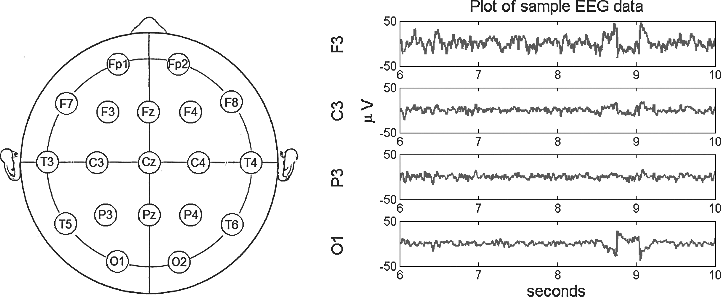
Left: A visualization of the international 10–20 system for electrode placement originally published in Jasper (1958). The present study only uses regions selected from the left hemisphere (Fp1, F7, F3, C3, P3, T3, T5, O1) and the right hemisphere (Fp2, F8, F4, C4, P4, T4, T6, O2), and excludes all midline sites. Right: A sample of 4 sec of resting EEG, recorded from channels F3, C3, P3, and O1.

Instantaneous phase

For a continuous time real valued process x_t, the analytic extension is defined as \documentclass{aastex}\usepackage{amsbsy}\usepackage{amsfonts}\usepackage{amssymb}\usepackage{bm}\usepackage{mathrsfs}\usepackage{pifont}\usepackage{stmaryrd}\usepackage{textcomp}\usepackage{portland, xspace}\usepackage{amsmath, amsxtra}\pagestyle{empty}\DeclareMathSizes{10}{9}{7}{6}\begin{document}\begin{align*}\chi_{t} = x_{t} + {i} \ \tilde{x}_{t} , \tag{1}\end{align*}\end{document}

where the integral is taken using the Cauchy principal value due to the potential singularity at \documentclass{aastex}\usepackage{amsbsy}\usepackage{amsfonts}\usepackage{amssymb}\usepackage{bm}\usepackage{mathrsfs}\usepackage{pifont}\usepackage{stmaryrd}\usepackage{textcomp}\usepackage{portland, xspace}\usepackage{amsmath, amsxtra}\pagestyle{empty}\DeclareMathSizes{10}{9}{7}{6}\begin{document}$$t = \tau$$\end{document} . Working with the analytic extension of the signal does not change the spectral density; however, additional information can be recovered using the tools of complex analysis. The instantaneous amplitude and phase are defined as the magnitude and argument of the analytic extension. For example if \documentclass{aastex}\usepackage{amsbsy}\usepackage{amsfonts}\usepackage{amssymb}\usepackage{bm}\usepackage{mathrsfs}\usepackage{pifont}\usepackage{stmaryrd}\usepackage{textcomp}\usepackage{portland, xspace}\usepackage{amsmath, amsxtra}\pagestyle{empty}\DeclareMathSizes{10}{9}{7}{6}\begin{document}$$\chi_{t}$$\end{document} is the analytic extension of the real valued signal x_t, then the instantaneous amplitude A_t and phase \documentclass{aastex}\usepackage{amsbsy}\usepackage{amsfonts}\usepackage{amssymb}\usepackage{bm}\usepackage{mathrsfs}\usepackage{pifont}\usepackage{stmaryrd}\usepackage{textcomp}\usepackage{portland, xspace}\usepackage{amsmath, amsxtra}\pagestyle{empty}\DeclareMathSizes{10}{9}{7}{6}\begin{document}$$\phi_{t}$$\end{document} are defined such that \documentclass{aastex}\usepackage{amsbsy}\usepackage{amsfonts}\usepackage{amssymb}\usepackage{bm}\usepackage{mathrsfs}\usepackage{pifont}\usepackage{stmaryrd}\usepackage{textcomp}\usepackage{portland, xspace}\usepackage{amsmath, amsxtra}\pagestyle{empty}\DeclareMathSizes{10}{9}{7}{6}\begin{document}\begin{align*}\chi_{t} = A_{t} e^{i \phi t} \tag{3}\end{align*}\end{document}

Conditions are given for a signal to have a physically meaningful interpretation of the instantaneous phase and amplitude (Chavez et al., 2006). In this study, the authors require that the signal be described by a small spectral band centered on the main frequency component, and that it satisfies the narrowband approximation, that is, it is one whose relative rate of change in amplitude is small compared with the rate of change in phase.

Complex demodulation is an algorithm for calculating the instantaneous phase of time series data (Bingham et al., 1967; Goodman, 1960). The original signal is transformed so that the relevant frequency band \documentclass{aastex}\usepackage{amsbsy}\usepackage{amsfonts}\usepackage{amssymb}\usepackage{bm}\usepackage{mathrsfs}\usepackage{pifont}\usepackage{stmaryrd}\usepackage{textcomp}\usepackage{portland, xspace}\usepackage{amsmath, amsxtra}\pagestyle{empty}\DeclareMathSizes{10}{9}{7}{6}\begin{document}$$( \omega - \delta , \omega + \delta )$$\end{document} is shifted to be centered at zero. The frequency shifted signal is calculated using the sine function, and a cosine function is used to calculate the frequency shifted Hilbert transform, \documentclass{aastex}\usepackage{amsbsy}\usepackage{amsfonts}\usepackage{amssymb}\usepackage{bm}\usepackage{mathrsfs}\usepackage{pifont}\usepackage{stmaryrd}\usepackage{textcomp}\usepackage{portland, xspace}\usepackage{amsmath, amsxtra}\pagestyle{empty}\DeclareMathSizes{10}{9}{7}{6}\begin{document}\begin{align*}y_{t} = {x}_{t} {\rm sin} ( - \omega t ) , \quad \tilde{y}_{t} = {x}_{t} \ {\rm cos} ( - \omega t ) , \tag{4}\end{align*}\end{document}

With the relevant frequencies shifted to 0, the analytic extension is put through a \documentclass{aastex}\usepackage{amsbsy}\usepackage{amsfonts}\usepackage{amssymb}\usepackage{bm}\usepackage{mathrsfs}\usepackage{pifont}\usepackage{stmaryrd}\usepackage{textcomp}\usepackage{portland, xspace}\usepackage{amsmath, amsxtra}\pagestyle{empty}\DeclareMathSizes{10}{9}{7}{6}\begin{document}$$\delta$$\end{document} Hz lowpass filter. The power remaining in the signal is the band \documentclass{aastex}\usepackage{amsbsy}\usepackage{amsfonts}\usepackage{amssymb}\usepackage{bm}\usepackage{mathrsfs}\usepackage{pifont}\usepackage{stmaryrd}\usepackage{textcomp}\usepackage{portland, xspace}\usepackage{amsmath, amsxtra}\pagestyle{empty}\DeclareMathSizes{10}{9}{7}{6}\begin{document}$$( \omega - \delta , \omega + \delta )$$\end{document} from the original signal. This process ensures that the resulting instantaneous phase can be meaningfully interpreted as the phase of the \documentclass{aastex}\usepackage{amsbsy}\usepackage{amsfonts}\usepackage{amssymb}\usepackage{bm}\usepackage{mathrsfs}\usepackage{pifont}\usepackage{stmaryrd}\usepackage{textcomp}\usepackage{portland, xspace}\usepackage{amsmath, amsxtra}\pagestyle{empty}\DeclareMathSizes{10}{9}{7}{6}\begin{document}$$( \omega - \delta , \omega + \delta )$$\end{document} component of the signal. The instantaneous amplitude and phase are calculated as, \documentclass{aastex}\usepackage{amsbsy}\usepackage{amsfonts}\usepackage{amssymb}\usepackage{bm}\usepackage{mathrsfs}\usepackage{pifont}\usepackage{stmaryrd}\usepackage{textcomp}\usepackage{portland, xspace}\usepackage{amsmath, amsxtra}\pagestyle{empty}\DeclareMathSizes{10}{9}{7}{6}\begin{document}\begin{align*}A_ {t} = \sqrt {y_ {t} ^ {2} + \tilde {y} _ {t} ^ {2}} , \quad \phi_ {t} = tan^ {- 1} \left( \frac {\tilde {y} _ {t}} {y_ {t}} \right) \tag {5} \end{align*}\end{document}

The time series of instantaneous phase values must undergo phase straightening to remove the discontinuities that exist due to tan⁻¹ function, a process that is particularly important for this application because the phase derivative must be estimated to identify periods of phase locking. 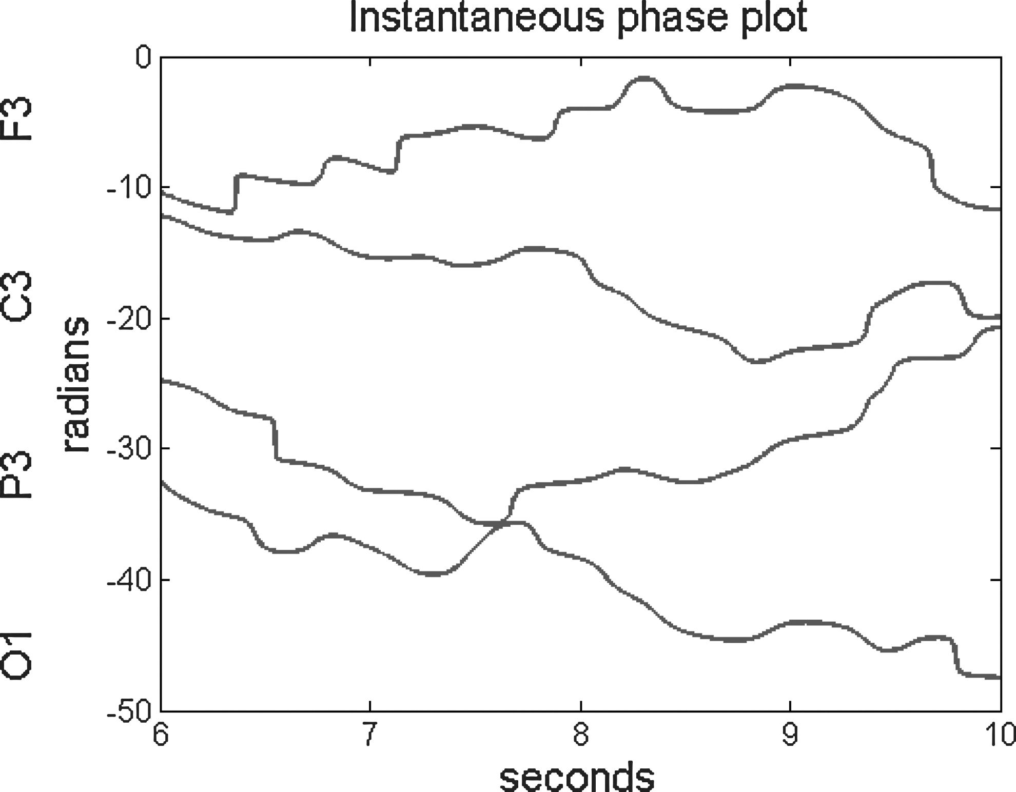Phase straightening is performed by searching for discontinuities in the instantaneous phase and, when one is found, adding or subtracting \documentclass{aastex}\usepackage{amsbsy}\usepackage{amsfonts}\usepackage{amssymb}\usepackage{bm}\usepackage{mathrsfs}\usepackage{pifont}\usepackage{stmaryrd}\usepackage{textcomp}\usepackage{portland, xspace}\usepackage{amsmath, amsxtra}\pagestyle{empty}\DeclareMathSizes{10}{9}{7}{6}\begin{document}$$2 \pi$$\end{document} based on the direction of the discontinuity. The estimated instantaneous phase in the 8–10 Hz band of the signals from the sample data are shown in Figure 2. The plot shows periods where the phase is approximately constant as well as sudden jumps in the instantaneous phase.

FIG. 2.

Instantaneous phase estimates of the four channels from Figure 1. There are two important features in these plots, a slight negative trend and sudden jumps in the phase. The sudden jumps are phase shift events. Many of the shift events are obvious, but there are some places where it is difficult to tell if there is a phase slip or just noise in the signal (for example, at the O1 signal just before 9 sec). This ambiguity is dealt with using an objective threshold technique (see Phase shifts section).

Phase synchrony

In the study of periodic oscillators, two oscillators with the same frequency are said to display phase synchrony if there is a constant relationship between phases (Boccaletti et al., 2002) \documentclass{aastex}\usepackage{amsbsy}\usepackage{amsfonts}\usepackage{amssymb}\usepackage{bm}\usepackage{mathrsfs}\usepackage{pifont}\usepackage{stmaryrd}\usepackage{textcomp}\usepackage{portland, xspace}\usepackage{amsmath, amsxtra}\pagestyle{empty}\DeclareMathSizes{10}{9}{7}{6}\begin{document}\begin{align*}\Phi_{t} = \mid \phi_{t}^{x} - \phi_{t}^{y} \mid = k , \ \forall t \tag{6}\end{align*}\end{document}

To identify periods of synchrony in the presence of noise, Breakspear's method (Breakspear et al., 2004) defines two signals as phase locked when their PDD is below a threshold value c \documentclass{aastex}\usepackage{amsbsy}\usepackage{amsfonts}\usepackage{amssymb}\usepackage{bm}\usepackage{mathrsfs}\usepackage{pifont}\usepackage{stmaryrd}\usepackage{textcomp}\usepackage{portland, xspace}\usepackage{amsmath, amsxtra}\pagestyle{empty}\DeclareMathSizes{10}{9}{7}{6}\begin{document}\begin{align*}\bigg | \frac {\Phi_ {t}} {dt} \bigg | < c , \, \forall t \tag {7} \end{align*}\end{document}

Phase locking has been used as a synonym for phase synchrony; at this point it is used to describe this specific measure of phase synchrony.

Phase shifts

When the PDD first exceeds the threshold value in phase locking analysis, there is said to be a phase shift between the coupled oscillators. In this study, they analyze these characteristic phase shift events outside the context of phase synchrony across channels. Rather than identifying shifts in the phase difference between two channels, phase shifts can be identified for each individual channel. If \documentclass{aastex}\usepackage{amsbsy}\usepackage{amsfonts}\usepackage{amssymb}\usepackage{bm}\usepackage{mathrsfs}\usepackage{pifont}\usepackage{stmaryrd}\usepackage{textcomp}\usepackage{portland, xspace}\usepackage{amsmath, amsxtra}\pagestyle{empty}\DeclareMathSizes{10}{9}{7}{6}\begin{document}$$\phi_{t}$$\end{document} represents the instantaneous phase of a time series, there is said to be a phase shift at time t if \documentclass{aastex}\usepackage{amsbsy}\usepackage{amsfonts}\usepackage{amssymb}\usepackage{bm}\usepackage{mathrsfs}\usepackage{pifont}\usepackage{stmaryrd}\usepackage{textcomp}\usepackage{portland, xspace}\usepackage{amsmath, amsxtra}\pagestyle{empty}\DeclareMathSizes{10}{9}{7}{6}\begin{document}\begin{align*}\mid \phi{\prime} _{t - 1} \mid < c , \ and \ \mid \phi{\prime} _{t} \mid > c , \tag{8}\end{align*}\end{document}

The method of using the phase derivative to identify shift events in the presence of noise may lead to false positives. As long as these false positives are in fact random and do not follow some spatiotemporal pattern, then they will not contribute to connectivity analysis; furthermore, a well selected value of the threshold parameter can help to reduce the number of false positive events. In previous studies, a simple visual inspection has been used to determine an appropriate value of c (Breakspear et al., 2004; Thatcher et al., 2009), but this includes an unwanted subjective aspect to the analysis. Note also that the appropriate range of values for c depend on properties of the signal such as the sampling rate, the filters applied and the frequency band of interest and, therefore, may differ from study to study. At this point, they select a threshold value in an objective manner, using the natural variability in the instantaneous phase signal to define a threshold which can adapt to different situations.

By estimating the variance of the instantaneous phase derivative \documentclass{aastex}\usepackage{amsbsy}\usepackage{amsfonts}\usepackage{amssymb}\usepackage{bm}\usepackage{mathrsfs}\usepackage{pifont}\usepackage{stmaryrd}\usepackage{textcomp}\usepackage{portland, xspace}\usepackage{amsmath, amsxtra}\pagestyle{empty}\DeclareMathSizes{10}{9}{7}{6}\begin{document}$$( \hat {\sigma} )$$\end{document} , and using the \documentclass{aastex}\usepackage{amsbsy}\usepackage{amsfonts}\usepackage{amssymb}\usepackage{bm}\usepackage{mathrsfs}\usepackage{pifont}\usepackage{stmaryrd}\usepackage{textcomp}\usepackage{portland, xspace}\usepackage{amsmath, amsxtra}\pagestyle{empty}\DeclareMathSizes{10}{9}{7}{6}\begin{document}$$1 - \alpha$$\end{document} quantile of the standard normal distribution \documentclass{aastex}\usepackage{amsbsy}\usepackage{amsfonts}\usepackage{amssymb}\usepackage{bm}\usepackage{mathrsfs}\usepackage{pifont}\usepackage{stmaryrd}\usepackage{textcomp}\usepackage{portland, xspace}\usepackage{amsmath, amsxtra}\pagestyle{empty}\DeclareMathSizes{10}{9}{7}{6}\begin{document}$$( z_{1 - \alpha} )$$\end{document} , a threshold value is determined which controls the rate of false positives ( \documentclass{aastex}\usepackage{amsbsy}\usepackage{amsfonts}\usepackage{amssymb}\usepackage{bm}\usepackage{mathrsfs}\usepackage{pifont}\usepackage{stmaryrd}\usepackage{textcomp}\usepackage{portland, xspace}\usepackage{amsmath, amsxtra}\pagestyle{empty}\DeclareMathSizes{10}{9}{7}{6}\begin{document}$$\alpha = 0.05$$\end{document} for their application) \documentclass{aastex}\usepackage{amsbsy}\usepackage{amsfonts}\usepackage{amssymb}\usepackage{bm}\usepackage{mathrsfs}\usepackage{pifont}\usepackage{stmaryrd}\usepackage{textcomp}\usepackage{portland, xspace}\usepackage{amsmath, amsxtra}\pagestyle{empty}\DeclareMathSizes{10}{9}{7}{6}\begin{document}\begin{align*}c = \hat{\sigma}z_{1 - \alpha} \tag{9}\end{align*}\end{document}

Phase shift events in the signal will artificially increase the estimated variance of the phase-locked instantaneous phase derivative, so as phase shift events are identified those points must be removed from the variance estimate. If the maximum value of \documentclass{aastex}\usepackage{amsbsy}\usepackage{amsfonts}\usepackage{amssymb}\usepackage{bm}\usepackage{mathrsfs}\usepackage{pifont}\usepackage{stmaryrd}\usepackage{textcomp}\usepackage{portland, xspace}\usepackage{amsmath, amsxtra}\pagestyle{empty}\DeclareMathSizes{10}{9}{7}{6}\begin{document}$$\mid \phi{\prime} _{t} \mid$$\end{document} exceeds the threshold value, each point above the threshold is removed from the set of phase-locked values, and then the variance (and threshold) are recalculated using only phase-locked values. The process is then recursively applied until the threshold converges to a fixed value (the estimated variance is positive and monotonically decreasing, so convergence to a non-negative threshold is guaranteed). Once the threshold has converged, a phase shift event is identified at the value of t which maximizes \documentclass{aastex}\usepackage{amsbsy}\usepackage{amsfonts}\usepackage{amssymb}\usepackage{bm}\usepackage{mathrsfs}\usepackage{pifont}\usepackage{stmaryrd}\usepackage{textcomp}\usepackage{portland, xspace}\usepackage{amsmath, amsxtra}\pagestyle{empty}\DeclareMathSizes{10}{9}{7}{6}\begin{document}$$\mid \phi{\prime} _{t} \mid$$\end{document} for each interval of time where \documentclass{aastex}\usepackage{amsbsy}\usepackage{amsfonts}\usepackage{amssymb}\usepackage{bm}\usepackage{mathrsfs}\usepackage{pifont}\usepackage{stmaryrd}\usepackage{textcomp}\usepackage{portland, xspace}\usepackage{amsmath, amsxtra}\pagestyle{empty}\DeclareMathSizes{10}{9}{7}{6}\begin{document}$$\mid \phi_{t}^{\prime} \mid$$\end{document} is above the threshold.

In this context, patterns in phase shift events can be analyzed in a multivariate model of EEG signals, taking into account events from across the scalp. Figure 3 shows the instantaneous phase derivative of the example data. A phase shift event occurs at the local maximum of the PDD.

FIG. 3.

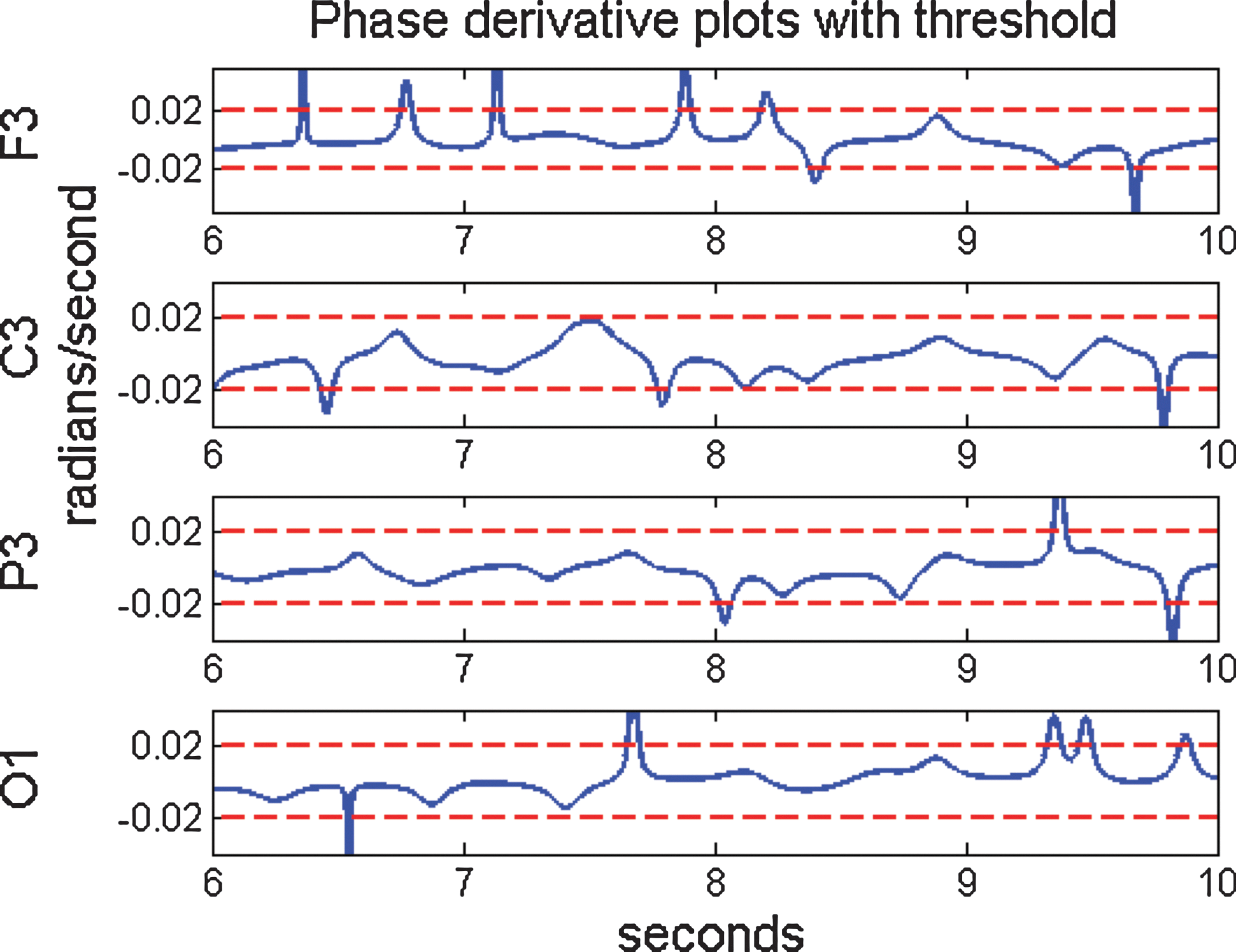
Plots of the phase derivative of the four instantaneous phase signals in Figure 2, including a dashed line indicating a threshold value of c=0.02. Notice that the deviations of the phase derivative of channel O1 just before 9 sec were not large enough to be classified as a phase shift. Color images available online at www.liebertpub.com/brain

Phase shift Granger causality

A point process is a model which describes the occurrence of random events localized in either time, space, or both. There are a number of equivalent ways to describe a point process; for a review of these and some other properties see Daley and Vere-Jones (2003). This document will only be concerned with temporal point processes, corresponding to events on the positive real line.

A continuous time point process is described by an integer-valued random step function N(t), defined to be the number of events which occur in the interval (0,t). A set of observed data from a point process, called a sample path, is an increasing sequence of numbers 0<t₁<t₂<…<t_K for some value of \documentclass{aastex}\usepackage{amsbsy}\usepackage{amsfonts}\usepackage{amssymb}\usepackage{bm}\usepackage{mathrsfs}\usepackage{pifont}\usepackage{stmaryrd}\usepackage{textcomp}\usepackage{portland, xspace}\usepackage{amsmath, amsxtra}\pagestyle{empty}\DeclareMathSizes{10}{9}{7}{6}\begin{document}$$K < \infty$$\end{document} , which defines the time of each event. A sample point process representation of phase shift events is shown in Figure 4. If the number of events in successive intervals is independent, the probability structure of a point process model can be completely described in terms of an inhomogeneous Poisson process with intensity function \documentclass{aastex}\usepackage{amsbsy}\usepackage{amsfonts}\usepackage{amssymb}\usepackage{bm}\usepackage{mathrsfs}\usepackage{pifont}\usepackage{stmaryrd}\usepackage{textcomp}\usepackage{portland, xspace}\usepackage{amsmath, amsxtra}\pagestyle{empty}\DeclareMathSizes{10}{9}{7}{6}\begin{document}\begin{align*}\lambda_ {t} = {\rm lim} _ {h \rightarrow 0} \frac {P ( N ( t + h ) - N ( t ) )} {h} . \tag {10} \end{align*}\end{document}

FIG. 4.

A visualization of the point process of phase shift events identified in Figure 3. Spatial and temporal patterns in these events are further analyzed using Granger causality in Phase Shift Granger Causality section.

When the number of events in successive intervals is not independent or depends on other variables, a conditional intensity function (CIF) can be used to describe the distribution of the process, \documentclass{aastex}\usepackage{amsbsy}\usepackage{amsfonts}\usepackage{amssymb}\usepackage{bm}\usepackage{mathrsfs}\usepackage{pifont}\usepackage{stmaryrd}\usepackage{textcomp}\usepackage{portland, xspace}\usepackage{amsmath, amsxtra}\pagestyle{empty}\DeclareMathSizes{10}{9}{7}{6}\begin{document}\begin{align*}\lambda_ {t} = {\rm lim} _ {h \rightarrow 0} \frac {P ( N ( t + h ) - N ( t ) = 1 \ \mid H_ {t} )} {h} . \tag {11} \end{align*}\end{document}

Now the term H_t is the complete history of the process up to but not including time t. The history can also include information from other processes or various exogenous variables. The CIF is interpreted as \documentclass{aastex}\usepackage{amsbsy}\usepackage{amsfonts}\usepackage{amssymb}\usepackage{bm}\usepackage{mathrsfs}\usepackage{pifont}\usepackage{stmaryrd}\usepackage{textcomp}\usepackage{portland, xspace}\usepackage{amsmath, amsxtra}\pagestyle{empty}\DeclareMathSizes{10}{9}{7}{6}\begin{document}\begin{align*}\lambda ( t ) dt \approx E ( N ( t + dt ) - N ( t ) \mid H_{t} ) . \tag{12}\end{align*}\end{document}

Exactly what information is in H_t and how it is incorporated into the CIF depends on the context of the problem.

For a recording with S channels, let N_i(t) (i=1.S) define the phase shift point process of the i^th signal. Following Kim and associates (2011), the history H_t will be the number of events R(t) in M consecutive nonoverlapping windows of length W that occur just before t. The history will also contain similar information for each signal in the recording, \documentclass{aastex}\usepackage{amsbsy}\usepackage{amsfonts}\usepackage{amssymb}\usepackage{bm}\usepackage{mathrsfs}\usepackage{pifont}\usepackage{stmaryrd}\usepackage{textcomp}\usepackage{portland, xspace}\usepackage{amsmath, amsxtra}\pagestyle{empty}\DeclareMathSizes{10}{9}{7}{6}\begin{document}\begin{align*}H_{t} = \{R_{i , m} \mid i = 1. S , m = 1. M \} \tag{13}\end{align*}\end{document}

The values R_i,m(t) are then be used to define a log-linear parameterization of the CIF for process N_j, \documentclass{aastex}\usepackage{amsbsy}\usepackage{amsfonts}\usepackage{amssymb}\usepackage{bm}\usepackage{mathrsfs}\usepackage{pifont}\usepackage{stmaryrd}\usepackage{textcomp}\usepackage{portland, xspace}\usepackage{amsmath, amsxtra}\pagestyle{empty}\DeclareMathSizes{10}{9}{7}{6}\begin{document}\begin{align*}log \lambda_{j} ( t ) = \gamma_{j , 0} + \mathop\sum \limits_{i , m}^{S , M} \gamma_{i , m} R_{i , m} ( t ) . \tag{15}\end{align*}\end{document}

The parameters \documentclass{aastex}\usepackage{amsbsy}\usepackage{amsfonts}\usepackage{amssymb}\usepackage{bm}\usepackage{mathrsfs}\usepackage{pifont}\usepackage{stmaryrd}\usepackage{textcomp}\usepackage{portland, xspace}\usepackage{amsmath, amsxtra}\pagestyle{empty}\DeclareMathSizes{10}{9}{7}{6}\begin{document}$$\gamma_{i}$$\end{document} , represent the effect that N_i has on the intensity of N_j.

Given a sample path \documentclass{aastex}\usepackage{amsbsy}\usepackage{amsfonts}\usepackage{amssymb}\usepackage{bm}\usepackage{mathrsfs}\usepackage{pifont}\usepackage{stmaryrd}\usepackage{textcomp}\usepackage{portland, xspace}\usepackage{amsmath, amsxtra}\pagestyle{empty}\DeclareMathSizes{10}{9}{7}{6}\begin{document}$$\{t_{1} , t_{2} , \ldots , t_{N_{j}} ( t ) \} $$\end{document} for channel N_j, the likelihood function for this model is given by \documentclass{aastex}\usepackage{amsbsy}\usepackage{amsfonts}\usepackage{amssymb}\usepackage{bm}\usepackage{mathrsfs}\usepackage{pifont}\usepackage{stmaryrd}\usepackage{textcomp}\usepackage{portland, xspace}\usepackage{amsmath, amsxtra}\pagestyle{empty}\DeclareMathSizes{10}{9}{7}{6}\begin{document}\begin{align*}L_{j} ( \vec{\gamma} ) = e^{- \int_{0}^{T} \lambda_{j} ( u ) du} \mathop\prod \limits_{i = 1}^{N_{j} ( T )} \lambda_{j} ( t_{i} ) . \tag{16}\end{align*}\end{document}

If the time interval is discretized into small bins of length \documentclass{aastex}\usepackage{amsbsy}\usepackage{amsfonts}\usepackage{amssymb}\usepackage{bm}\usepackage{mathrsfs}\usepackage{pifont}\usepackage{stmaryrd}\usepackage{textcomp}\usepackage{portland, xspace}\usepackage{amsmath, amsxtra}\pagestyle{empty}\DeclareMathSizes{10}{9}{7}{6}\begin{document}$$\Delta$$\end{document} , and \documentclass{aastex}\usepackage{amsbsy}\usepackage{amsfonts}\usepackage{amssymb}\usepackage{bm}\usepackage{mathrsfs}\usepackage{pifont}\usepackage{stmaryrd}\usepackage{textcomp}\usepackage{portland, xspace}\usepackage{amsmath, amsxtra}\pagestyle{empty}\DeclareMathSizes{10}{9}{7}{6}\begin{document}$$\Delta$$\end{document} is chosen such that the probability of two or more events in a single bin is negligible, \documentclass{aastex}\usepackage{amsbsy}\usepackage{amsfonts}\usepackage{amssymb}\usepackage{bm}\usepackage{mathrsfs}\usepackage{pifont}\usepackage{stmaryrd}\usepackage{textcomp}\usepackage{portland, xspace}\usepackage{amsmath, amsxtra}\pagestyle{empty}\DeclareMathSizes{10}{9}{7}{6}\begin{document}\begin{align*}P ( N_{j} ( t + \Delta ) - N_{j} ( t ) \ge 2 ) \approx 0 , \tag{17}\end{align*}\end{document}

then the likelihood function can be approximated as a product of independent nonidentical Bernoulli trials (Daley and Vere-Jones, 2003). They define dN(t_k) as the number of events in the k^th bin, that is \documentclass{aastex}\usepackage{amsbsy}\usepackage{amsfonts}\usepackage{amssymb}\usepackage{bm}\usepackage{mathrsfs}\usepackage{pifont}\usepackage{stmaryrd}\usepackage{textcomp}\usepackage{portland, xspace}\usepackage{amsmath, amsxtra}\pagestyle{empty}\DeclareMathSizes{10}{9}{7}{6}\begin{document}\begin{align*}dN_{j} ( t_{k} ) = N_{j} ( t_{k} ) - N_{j} ( t_{k} - \Delta ) , \ k = 1..K \tag{18}\end{align*}\end{document}

then, \documentclass{aastex}\usepackage{amsbsy}\usepackage{amsfonts}\usepackage{amssymb}\usepackage{bm}\usepackage{mathrsfs}\usepackage{pifont}\usepackage{stmaryrd}\usepackage{textcomp}\usepackage{portland, xspace}\usepackage{amsmath, amsxtra}\pagestyle{empty}\DeclareMathSizes{10}{9}{7}{6}\begin{document}\begin{align*}L_{j} ( \vec{\gamma} ) = \mathop\prod \limits_{k = 1}^{K} ( \lambda_{j} ( t_{k} ) \Delta ) ^{dN_{j} ( t_{k} ) - 1} ( 1 - \lambda_{j} ( t_{k} ) \Delta ) ^{1 - dN_{j} ( t_{k} )}. \tag{20}\end{align*}\end{document}

This approximation is particularly useful because it leads to a convex likelihood function, allowing easy access to the maximum likelihood estimates of the parameters. A standard Newton's method (Atkinson, 1989) was used to find the maximum likelihood estimates for the parameters; for computational reasons a lower bound on parameters of −10 was included in the estimation.

An important aspect of Granger causality measures is the ability to test the hypothesis “N_i does not Granger cause N_j”. By comparing the full likelihood for N_j with a reduced likelihood with the history of N_i removed \documentclass{aastex}\usepackage{amsbsy}\usepackage{amsfonts}\usepackage{amssymb}\usepackage{bm}\usepackage{mathrsfs}\usepackage{pifont}\usepackage{stmaryrd}\usepackage{textcomp}\usepackage{portland, xspace}\usepackage{amsmath, amsxtra}\pagestyle{empty}\DeclareMathSizes{10}{9}{7}{6}\begin{document}$$( R_{i , ^{.}} ( t ) )$$\end{document} , one can test whether the information in N_i causes a significant reduction in the prediction error. To determine the effect of the signal N_i on the optimal predictor for N_j, a reduced likelihood function is defined excluding the parameters \documentclass{aastex}\usepackage{amsbsy}\usepackage{amsfonts}\usepackage{amssymb}\usepackage{bm}\usepackage{mathrsfs}\usepackage{pifont}\usepackage{stmaryrd}\usepackage{textcomp}\usepackage{portland, xspace}\usepackage{amsmath, amsxtra}\pagestyle{empty}\DeclareMathSizes{10}{9}{7}{6}\begin{document}$$\gamma_{i}$$\end{document} , from the CIF \documentclass{aastex}\usepackage{amsbsy}\usepackage{amsfonts}\usepackage{amssymb}\usepackage{bm}\usepackage{mathrsfs}\usepackage{pifont}\usepackage{stmaryrd}\usepackage{textcomp}\usepackage{portland, xspace}\usepackage{amsmath, amsxtra}\pagestyle{empty}\DeclareMathSizes{10}{9}{7}{6}\begin{document}\begin{align*}log \lambda_{i , j}^* ( t ) = \gamma_{0} + \mathop\sum \limits_{m} \mathop\sum \limits_{q \neq i} \gamma_{q , m} R_{q , m} ( t ) . \tag{21}\end{align*}\end{document} \documentclass{aastex}\usepackage{amsbsy}\usepackage{amsfonts}\usepackage{amssymb}\usepackage{bm}\usepackage{mathrsfs}\usepackage{pifont}\usepackage{stmaryrd}\usepackage{textcomp}\usepackage{portland, xspace}\usepackage{amsmath, amsxtra}\pagestyle{empty}\DeclareMathSizes{10}{9}{7}{6}\begin{document}\begin{align*}L_{i , j}^* ( \vec{\gamma} ) = \mathop\prod \limits_{k = 1}^{K} ( \lambda_{i , j}^* ( t_{k} ) \Delta ) ^{dN_{j} ( t_{k} ) - 1} ( 1 - \lambda_{i , j}^* ( t_{k} ) \Delta ) ^{1 - d N_{j} ( t_{k} )} \tag{22}\end{align*}\end{document}

The likelihood ratio of the full and reduced models is used to define PSGC \documentclass{aastex}\usepackage{amsbsy}\usepackage{amsfonts}\usepackage{amssymb}\usepackage{bm}\usepackage{mathrsfs}\usepackage{pifont}\usepackage{stmaryrd}\usepackage{textcomp}\usepackage{portland, xspace}\usepackage{amsmath, amsxtra}\pagestyle{empty}\DeclareMathSizes{10}{9}{7}{6}\begin{document}$$\Phi_{i , j}$$\end{document} , an asymmetric measure of connectivity from N_i to N_j, \documentclass{aastex}\usepackage{amsbsy}\usepackage{amsfonts}\usepackage{amssymb}\usepackage{bm}\usepackage{mathrsfs}\usepackage{pifont}\usepackage{stmaryrd}\usepackage{textcomp}\usepackage{portland, xspace}\usepackage{amsmath, amsxtra}\pagestyle{empty}\DeclareMathSizes{10}{9}{7}{6}\begin{document}\begin{align*}\Phi_ {i , j} = - 2 \ {\rm log} \left( \frac {L_ {i , j} ^*} {L_ {j}} \right) \tag {23} \end{align*}\end{document}

To assess the significance of the PSGC measure, a natural hypothesis test exists in the form of a likelihood ratio test (LRT). For large values of T the values \documentclass{aastex}\usepackage{amsbsy}\usepackage{amsfonts}\usepackage{amssymb}\usepackage{bm}\usepackage{mathrsfs}\usepackage{pifont}\usepackage{stmaryrd}\usepackage{textcomp}\usepackage{portland, xspace}\usepackage{amsmath, amsxtra}\pagestyle{empty}\DeclareMathSizes{10}{9}{7}{6}\begin{document}$$\Phi_{i , j}$$\end{document} follow an approximate chi-squared distribution with M degrees of freedom, \documentclass{aastex}\usepackage{amsbsy}\usepackage{amsfonts}\usepackage{amssymb}\usepackage{bm}\usepackage{mathrsfs}\usepackage{pifont}\usepackage{stmaryrd}\usepackage{textcomp}\usepackage{portland, xspace}\usepackage{amsmath, amsxtra}\pagestyle{empty}\DeclareMathSizes{10}{9}{7}{6}\begin{document}\begin{align*}\Phi_{i , j} \, \sim \, \chi^{2} ( M ) \tag{24}\end{align*}\end{document}

This provides a test for Granger causality from N_i to N_j within the framework of a multivariate model of the signals, meaning that the test is able to account for common information contained in multiple signals. If N_i is estimated to Granger-cause N_j, then knowledge of past shift events in N_i improves prediction of future shift events in N_j. In other words, if there is a shift at N_i, then it will either increase or decrease the probability that N_j will shift in the imminent future.

As an additional method of statistical validation of the results, a group level analysis can be applied to unordered pairs of signals to test the hypothesis of zero net Granger causality. This is achieved using the method of time-reversed surrogate data from Haufe and associates (2013). Since the degrees of freedom (M) may change for each dataset (participant), PSGC scores were converted to p-values, and then an inverse transformation was used to generate values from a \documentclass{aastex}\usepackage{amsbsy}\usepackage{amsfonts}\usepackage{amssymb}\usepackage{bm}\usepackage{mathrsfs}\usepackage{pifont}\usepackage{stmaryrd}\usepackage{textcomp}\usepackage{portland, xspace}\usepackage{amsmath, amsxtra}\pagestyle{empty}\DeclareMathSizes{10}{9}{7}{6}\begin{document}$$\chi^{2} ( 4 )$$\end{document} distribution. A statistic is calculated to quantify the net GC by looking at the difference between asymmetric causality scores in the forward and time-reversed data, \documentclass{aastex}\usepackage{amsbsy}\usepackage{amsfonts}\usepackage{amssymb}\usepackage{bm}\usepackage{mathrsfs}\usepackage{pifont}\usepackage{stmaryrd}\usepackage{textcomp}\usepackage{portland, xspace}\usepackage{amsmath, amsxtra}\pagestyle{empty}\DeclareMathSizes{10}{9}{7}{6}\begin{document}\begin{align*}d_{k} = \left( \Phi_{i , j}^{( k )} - \Phi_{j , i}^{( k )} \right) - \left( T R \Phi_{i , j}^{( k )} - T R \Phi_{j , i}^{( k )} \right) \tag{25}\end{align*}\end{document}

The null hypothesis of zero net connectivity \documentclass{aastex}\usepackage{amsbsy}\usepackage{amsfonts}\usepackage{amssymb}\usepackage{bm}\usepackage{mathrsfs}\usepackage{pifont}\usepackage{stmaryrd}\usepackage{textcomp}\usepackage{portland, xspace}\usepackage{amsmath, amsxtra}\pagestyle{empty}\DeclareMathSizes{10}{9}{7}{6}\begin{document}$$( \mu_{d} = 0 )$$\end{document} is tested using a standard t-test. Since the time-reversed data maintain most of the underlying structure of the original signal, the test for net GC is not sensitive to the so-called weak asymmetries (Haufe et al. 2013) such as those induced by volume conduction. They will subsequently refer to this second statistical test as a net GC analysis.

Application details

In this article, they applied the PSGC method in a proof-of-concept simulation study (Proof of concept section) as well as to real EEG recordings of resting and vigilance tasks (Functional application section). Now they describe the specific details of the implementation of the PSGC method for both the real and simulated applications.

Based on the results of previous analysis of the EEG tasks using phase reset measures and their association with individual difference variables (Lackner et al., 2014), the frequency band of interest for these analyses was 8–10 Hz. The instantaneous phase of each channel was calculated by shifting the centre of the band of interest to 0 Hz and then putting the result through a 1 Hz low-pass Butterworth filter.

For the point process model, the length of the history windows W must be chosen so that the time scale is appropriate in the context of behavioral analysis. For this study, a value of W=100 ms was used. This value of W is approximately the length of a complete cycle at the frequency band of interest. For each recording (real and simulated data) and each channel, model selection was performed to select the optimal order M for the log-linear parameterization. The optimal value was determined by calculating the Akaike information criterion (Akaike, 1974) for a range of values of M (1 to 6) and selecting the one which minimized the criteria. This process creates a balance between goodness of fit and overparameterization of the model. In the EEG application, the optimal values of the order parameter M ranged from 3 to 5, corresponding to a total history length of 300–500 ms, which is enough time to capture a decision-making process.

Results for both statistical analyses were corrected for multiple comparisons using the Holm-Bonferroni procedure (Holm, 1979) to give a familywise error rate of \documentclass{aastex}\usepackage{amsbsy}\usepackage{amsfonts}\usepackage{amssymb}\usepackage{bm}\usepackage{mathrsfs}\usepackage{pifont}\usepackage{stmaryrd}\usepackage{textcomp}\usepackage{portland, xspace}\usepackage{amsmath, amsxtra}\pagestyle{empty}\DeclareMathSizes{10}{9}{7}{6}\begin{document}$$\alpha = 0.05$$\end{document} per hemisphere. For individual networks estimated using the LRT, corrections are applied based on (8×7)=56 comparisons per hemisphere and (8×7)/2=28 multiple comparisons for the net GC analysis.

Proof of Concept

Due to the nature of EEG recordings, there are a number of concerns to be addressed when performing connectivity analysis (Nolte et al., 2004). At any point in time, the EEG signal is a linear combination of the activity at each source. The conductive properties of the scalp instantly create attenuated versions of source activity at every scalp electrode, a process known as volume conduction. In studies of coherence, volume conduction can create artificially inflated coherence between distant electrodes (Nunez et al., 1997). Another consideration is that noise is a prominent feature of EEG recordings. Any method which is suitable for connectivity analysis should be able to detect it in the presence of noise and should not be affected by volume conduction.

To verify that the PSGC method is appropriate for EEG analysis, they performed simulations of simple oscillators with coupled phase shift behavior. The data were then transformed with a realistic lead field matrix to emulate the linear mixing characteristics of EEG. Simulations were performed for several levels of coupling strength, biological and measurement noise, to identify the range of behaviors for which the PSGC method reliably identifies connectivity.

Simulated data

Simulated data were generated from two oscillators located under the F4 and O2 scalp regions at a depth of 15% below the scalp, each with a 9 Hz component of interest. The phase of each oscillator was generated as \documentclass{aastex}\usepackage{amsbsy}\usepackage{amsfonts}\usepackage{amssymb}\usepackage{bm}\usepackage{mathrsfs}\usepackage{pifont}\usepackage{stmaryrd}\usepackage{textcomp}\usepackage{portland, xspace}\usepackage{amsmath, amsxtra}\pagestyle{empty}\DeclareMathSizes{10}{9}{7}{6}\begin{document}\begin{align*}\phi_{i , t} = \phi_{i , t - 1} + \epsilon_{i , t} \eta_{i , t} , \ i = \{F4 , O2 \} \tag{26}\end{align*}\end{document}

where \documentclass{aastex}\usepackage{amsbsy}\usepackage{amsfonts}\usepackage{amssymb}\usepackage{bm}\usepackage{mathrsfs}\usepackage{pifont}\usepackage{stmaryrd}\usepackage{textcomp}\usepackage{portland, xspace}\usepackage{amsmath, amsxtra}\pagestyle{empty}\DeclareMathSizes{10}{9}{7}{6}\begin{document}$$\epsilon_{i , t}$$\end{document} are binary variables which determine whether or not a phase shift occurs and \documentclass{aastex}\usepackage{amsbsy}\usepackage{amsfonts}\usepackage{amssymb}\usepackage{bm}\usepackage{mathrsfs}\usepackage{pifont}\usepackage{stmaryrd}\usepackage{textcomp}\usepackage{portland, xspace}\usepackage{amsmath, amsxtra}\pagestyle{empty}\DeclareMathSizes{10}{9}{7}{6}\begin{document}$$\eta_{i , t}$$\end{document} are independent random variables drawn from a \documentclass{aastex}\usepackage{amsbsy}\usepackage{amsfonts}\usepackage{amssymb}\usepackage{bm}\usepackage{mathrsfs}\usepackage{pifont}\usepackage{stmaryrd}\usepackage{textcomp}\usepackage{portland, xspace}\usepackage{amsmath, amsxtra}\pagestyle{empty}\DeclareMathSizes{10}{9}{7}{6}\begin{document}$$N \left( \frac {3 \pi} {5} , \frac {\pi} {5} \right)$$\end{document} distribution, which represent the phase shift magnitude. Each generator had a fixed probability of a shift event occurring ( \documentclass{aastex}\usepackage{amsbsy}\usepackage{amsfonts}\usepackage{amssymb}\usepackage{bm}\usepackage{mathrsfs}\usepackage{pifont}\usepackage{stmaryrd}\usepackage{textcomp}\usepackage{portland, xspace}\usepackage{amsmath, amsxtra}\pagestyle{empty}\DeclareMathSizes{10}{9}{7}{6}\begin{document}$$\gamma_{i}$$\end{document} ), unless the generator was in a brief refractory period, which occurred after each shift. The refractory period was 500 ms (approximately 5 cycles of 9 Hz) and it represents signal propagation and the formation of a neural assembly. To include information flow into the model, coupling parameters were used to increase the rate of phase shift events in the receiving generator for a period after each shift at a driving generator. Defining \documentclass{aastex}\usepackage{amsbsy}\usepackage{amsfonts}\usepackage{amssymb}\usepackage{bm}\usepackage{mathrsfs}\usepackage{pifont}\usepackage{stmaryrd}\usepackage{textcomp}\usepackage{portland, xspace}\usepackage{amsmath, amsxtra}\pagestyle{empty}\DeclareMathSizes{10}{9}{7}{6}\begin{document}$$\bar{\epsilon}_{i , t}$$\end{document} as the number of shifts at generator i which have occurred in the previous 500 ms, the probability of a phase shift is given by \documentclass{aastex}\usepackage{amsbsy}\usepackage{amsfonts}\usepackage{amssymb}\usepackage{bm}\usepackage{mathrsfs}\usepackage{pifont}\usepackage{stmaryrd}\usepackage{textcomp}\usepackage{portland, xspace}\usepackage{amsmath, amsxtra}\pagestyle{empty}\DeclareMathSizes{10}{9}{7}{6}\begin{document}\begin{align*}P ( \epsilon_{i , t} = 1 ) = \begin{cases} \gamma_{i} \quad \quad \quad \quad \quad \quad if \quad \bar{\epsilon}_{i , t} = 0 , \quad \bar{\epsilon}_{\backslash i , t} = 0 \\ \gamma_{i} + C_{i} \quad \quad \quad \quad if \quad \bar{\epsilon}_{i , t} = 0 , \quad \bar{\epsilon}_{\backslash i , t} = 1 \\ 0 \quad \quad \quad \quad \quad \quad \quad \quad \quad \quad \quad \quad otherwise\end{cases} \tag{27}\end{align*}\end{document}

where \i represents the driving generator. For these simulations they set the base rate of shifting to \documentclass{aastex}\usepackage{amsbsy}\usepackage{amsfonts}\usepackage{amssymb}\usepackage{bm}\usepackage{mathrsfs}\usepackage{pifont}\usepackage{stmaryrd}\usepackage{textcomp}\usepackage{portland, xspace}\usepackage{amsmath, amsxtra}\pagestyle{empty}\DeclareMathSizes{10}{9}{7}{6}\begin{document}$$\gamma_{i} = 0.0024$$\end{document} or approximately one shift every 0.83 sec. At this point the authors were primarily interested in the ability to identify an asymmetric coupling from the generator under F4 to the generator under O2 ( \documentclass{aastex}\usepackage{amsbsy}\usepackage{amsfonts}\usepackage{amssymb}\usepackage{bm}\usepackage{mathrsfs}\usepackage{pifont}\usepackage{stmaryrd}\usepackage{textcomp}\usepackage{portland, xspace}\usepackage{amsmath, amsxtra}\pagestyle{empty}\DeclareMathSizes{10}{9}{7}{6}\begin{document}$$C_{F4} = 0 , C_{O2} > 0$$\end{document} ).

Once instantaneous phase values were randomly generated, they were then converted to oscillators with unit amplitude, frequency f=9, and sampling rate T=500 Hz, \documentclass{aastex}\usepackage{amsbsy}\usepackage{amsfonts}\usepackage{amssymb}\usepackage{bm}\usepackage{mathrsfs}\usepackage{pifont}\usepackage{stmaryrd}\usepackage{textcomp}\usepackage{portland, xspace}\usepackage{amsmath, amsxtra}\pagestyle{empty}\DeclareMathSizes{10}{9}{7}{6}\begin{document}\begin{align*}x_ {i , t} = {\rm sin} \left( \frac {2 \pi f t} {T} + \phi_ {i , t} \right). \tag {28} \end{align*}\end{document}

The signals ( \documentclass{aastex}\usepackage{amsbsy}\usepackage{amsfonts}\usepackage{amssymb}\usepackage{bm}\usepackage{mathrsfs}\usepackage{pifont}\usepackage{stmaryrd}\usepackage{textcomp}\usepackage{portland, xspace}\usepackage{amsmath, amsxtra}\pagestyle{empty}\DeclareMathSizes{10}{9}{7}{6}\begin{document}$$X_{t} = [ x_{F4 , t} , x_{O2 , t} ]$$\end{document} from the generators were then linearly mixed to scalp electrodes using a realistic lead field matrix (A_x) with the generators constrained to be perpendicular to the scalp (Mosher et al., 1999). Sample scalp topographies for the simulated data are shown in Figure 5, \documentclass{aastex}\usepackage{amsbsy}\usepackage{amsfonts}\usepackage{amssymb}\usepackage{bm}\usepackage{mathrsfs}\usepackage{pifont}\usepackage{stmaryrd}\usepackage{textcomp}\usepackage{portland, xspace}\usepackage{amsmath, amsxtra}\pagestyle{empty}\DeclareMathSizes{10}{9}{7}{6}\begin{document}\begin{align*}S_{t} = A_{x} X_{t}. \tag{29}\end{align*}\end{document}

FIG. 5.

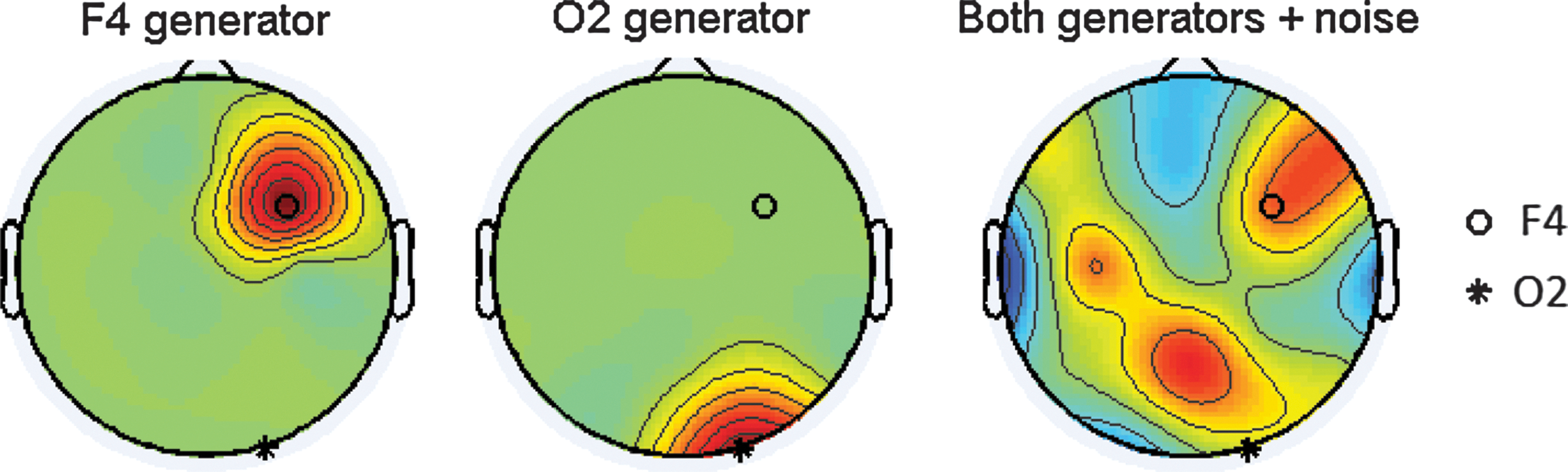
Scalp topographies of the two generators (Left: F4, Center: O2) and then both generators with the inclusion of spatial/temporal and measurement noise. Although the simulation study is performed solely on the right hemisphere sites, a full montage of 10–20 electrodes with measurement noise is used to generate these topographies. All topographies were taken at time t=1, a SNR of 0 dB (r_m=0.5), a bSNR of −4.8 dB (r_b=0.25) and were generated using EEGlab (Delorme and Makeig, 2004).

Following closely with Haufe and associates (2013), different types of noise were included in the simulations; however, now they defined separate parameters to control levels of biological signal-to-noise ratio (bSNR: r_b in [0,1]) and measurement signal-to-noise ratio (SNR: r_m in [0,1]). Independent measurement noise (E_t) was simulated from a N(0,1) distribution for each sensor. Additionally, several spatiotemporal sources of biological noise (n_i,t) were generated using temporally correlated AR noise. The noise sources were generated from AR(10) processes, with coefficients independently drawn from a N(0, 0.01) distribution. Spatial locations for the biological noise (N_biol,t=[n_1,t, n_2,t,…n_10,t]) were uniformly drawn from each hemisphere (five on the right, five on the left) with depths selected uniformly from 15% to 40% of the head model radius. The biological noise was then linearly mixed to the same scalp locations using a matrix A_n, which was calculated using the same method as A_x, \documentclass{aastex}\usepackage{amsbsy}\usepackage{amsfonts}\usepackage{amssymb}\usepackage{bm}\usepackage{mathrsfs}\usepackage{pifont}\usepackage{stmaryrd}\usepackage{textcomp}\usepackage{portland, xspace}\usepackage{amsmath, amsxtra}\pagestyle{empty}\DeclareMathSizes{10}{9}{7}{6}\begin{document}\begin{align*}N_{t} = A_{n} N_{biol , t} \tag{30}\end{align*}\end{document}

The signal and biological noise were scaled to have the specified contributions to the overall biological signal, \documentclass{aastex}\usepackage{amsbsy}\usepackage{amsfonts}\usepackage{amssymb}\usepackage{bm}\usepackage{mathrsfs}\usepackage{pifont}\usepackage{stmaryrd}\usepackage{textcomp}\usepackage{portland, xspace}\usepackage{amsmath, amsxtra}\pagestyle{empty}\DeclareMathSizes{10}{9}{7}{6}\begin{document}\begin{align*}B_ {t} = \frac {r_ {b} S_ {t}} {\big| \mid vec ( S_ {t} ) \mid \big|} + \frac {( 1 - r_ {b} ) N_ {t}} {\big| \mid vec ( N_ {t} ) \mid \big|} \tag {31} \end{align*}\end{document}

The overall biological signal B_t and measurement noise E_t were both normalized and the SNR was set in the observed data Y_t using a weighted combination of the two, \documentclass{aastex}\usepackage{amsbsy}\usepackage{amsfonts}\usepackage{amssymb}\usepackage{bm}\usepackage{mathrsfs}\usepackage{pifont}\usepackage{stmaryrd}\usepackage{textcomp}\usepackage{portland, xspace}\usepackage{amsmath, amsxtra}\pagestyle{empty}\DeclareMathSizes{10}{9}{7}{6}\begin{document}\begin{align*}Y_ {t} = \frac {r_ {m} B_ {t}} {\big| \mid vec ( B_ {t} ) \mid \big|} + \frac {( 1 - r_ {m} ) E_ {t}} {\big| \mid vec ( E_ {t} ) \mid \big|} . \tag {32} \end{align*}\end{document}

All sources were mixed to 128 scalp sites (EGI, Eugene, OR) referenced to Cz and then re-referenced to the average, to be consistent with the preprocessing applied in the application to real EEG data. Data were then reduced to eight channels at the right hemisphere locations (Fp2, F4, C4, P4, O2, F8, T4, T6) for the PSGC analysis.

Simulation results

Simulations were performed with three kinds of coupling (none, directed, feedback) over a range of bSNR. Preliminary results suggested that independent measurement noise does not contribute strongly to PSGC results so the SNR was set to a fixed 0 dB (r_m=0.5) for all simulations. For each set of parameters, 18 datasets were generated (to match the 18 participants in the application to real data). Simulated datasets were 5 min in length for the no-coupling and directed-coupling scenarios. Simulations of the feedback scenario were 10 min in length, as it was necessary to increase the power of the PSGC measure to identify this more complex dynamic. Specific details of how the PSGC analysis was conducted are described in the application details section.

The results of the PSGC analysis for all possible pairs of connections are summarized in Figure 6 for several sets of parameters. Each cell of the matrix represents the Granger causality from one signal to another. The i,j element of the matrix represents PSGC from N_j to N_i. The shade of each cell represents the number of simulations which found significant connectivity in the specified pathway. The i,j element is white if causality exists in every participant, black if there is causality in zero participants and shades of grey represent intermediate results. The diagonal entries are crossed out to emphasize that there is no analysis on these locations. Panels A and B show the results of simulations with asymmetric coupling (C_F4=0, C_O2=0.015) simulated with bSNRs of −12.8 dB (r_b=0.05) and −4.8 dB (and r_b=0.25). At the lowest bSNR, true connectivity \documentclass{aastex}\usepackage{amsbsy}\usepackage{amsfonts}\usepackage{amssymb}\usepackage{bm}\usepackage{mathrsfs}\usepackage{pifont}\usepackage{stmaryrd}\usepackage{textcomp}\usepackage{portland, xspace}\usepackage{amsmath, amsxtra}\pagestyle{empty}\DeclareMathSizes{10}{9}{7}{6}\begin{document}$$( F4 \rightarrow O2 )$$\end{document} is identified in over 50% of simulations, whereas for higher bSNRs the true connectivity is identified over 90% of the time. At both bSNR levels there are minimal false positives otherwise (never in more than 1 of the 18 simulations for a given pathway). Panels C and D show the results of simulations with no coupling (C_F4=C_O2=0), there are minimal connections identified; for bSNR levels of −4.8 dB and lower, the number of spurious connections which are identified are in line with the number of false positives they expect across many simulations.

FIG. 6.

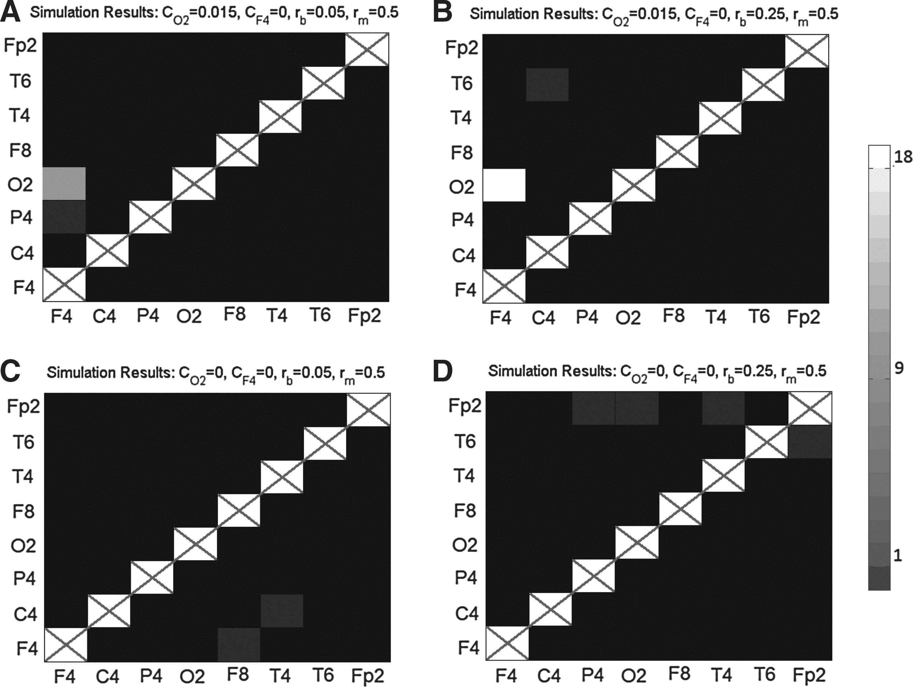
Each cell of the matrix represents the Granger causality from one signal to another. The i,j element of the matrix represents PSGC from N_i to N_j. The shade of each cell (see colorbar) represents the number of simulations which found significant connectivity in the specified pathway. (A, B) show the results of simulations with asymmetric coupling (C_F4=0, C_O2=0.015); at bSNRs −4.8 dB (and r_b=0.25) the true connectivity is identified over 90% of the time ( \documentclass{aastex}\usepackage{amsbsy}\usepackage{amsfonts}\usepackage{amssymb}\usepackage{bm}\usepackage{mathrsfs}\usepackage{pifont}\usepackage{stmaryrd}\usepackage{textcomp}\usepackage{portland, xspace}\usepackage{amsmath, amsxtra}\pagestyle{empty}\DeclareMathSizes{10}{9}{7}{6}\begin{document}$$F4 \rightarrow O2$$\end{document} ) and there are minimal false positives, otherwise (never in more than 1 of the 18 simulations for a given pathway). (C, D) show the results of simulations with no coupling (C_F4=C_O2=0), where there are minimal spurious connections.

They further explored the relationship between bSNR and PSGC by looking at the connectivity rates for two specific connections of interest \documentclass{aastex}\usepackage{amsbsy}\usepackage{amsfonts}\usepackage{amssymb}\usepackage{bm}\usepackage{mathrsfs}\usepackage{pifont}\usepackage{stmaryrd}\usepackage{textcomp}\usepackage{portland, xspace}\usepackage{amsmath, amsxtra}\pagestyle{empty}\DeclareMathSizes{10}{9}{7}{6}\begin{document}$$( F4 \rightarrow O2 \ and \ O2 \rightarrow F4 )$$\end{document} Figure 7 shows plots of the connectivity rates as a function of bSNR for simulations with no coupling (C_F4=C_O2=0), directed coupling (C_F4=0, C_O2=0.015), and feedback (C_F4=C_O2=0.015). In the left panel they see that the PSGC measure has a power of 80% or more to identify the true directed connection, power of up to 50% to identify the feedback connection, and in the uncoupled case they see no false positives for bSNR values up to −4.8 dB (r_b=0.25). In the right panel, they saw the same power to identify feedback connectivity, but only a single spurious connection in both the no-coupling and directed-coupling cases for bSNR levels of −4.8 dB (r_b=0.25) or lower. The reduced power to identify feedback connectivity is a direct result of the use of GC analysis; as the feedback connection becomes stronger, the two signals become entangled and it becomes difficult to completely remove the effect of F4 (or O2) from the model. For bSNR values greater than −2.7 dB (r_b=0.35), an unrealistically high level for continuous EEG recordings (see Volume conduction, reference electrode, and stationarity section), the results show larger amounts of spurious connectivity across many electrodes. This increase in spurious connectivity is likely due to a combination of volume conduction and average reference effects. The relationship between bSNR and the spread of phase shift events due to volume conduction and average reference is further quantified in Supplementary Section S2 (Supplementary Data are available online at www.liebertpub.com/brain). As the amount of true signal in the overall activity increases, it starts to dominate the average, and shift events in the true signal will be spread across the scalp through the average reference. This result suggests that the PSGC measure is appropriate for estimating connectivity in situations with low bSNR, but may not be accurate in high bSNR situations, such as when using averaged trials in event-related potential (ERP) analysis. Now they restrict their application to nonaveraged data, where low bSNRs are ubiquitous.

FIG. 7.

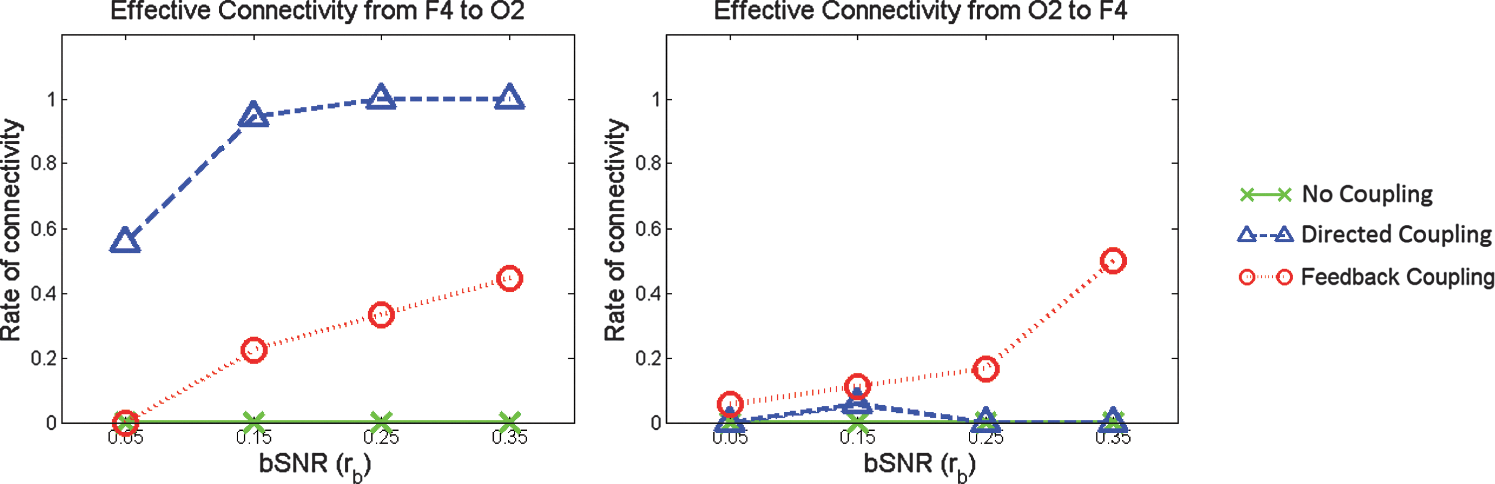
Plots of the connectivity rates as a function of bSNR for simulations with no coupling, directed coupling and bidirectional coupling. In the left panel they see that the PSGC measure has a power of 90% or more to identify a true directed connection \documentclass{aastex}\usepackage{amsbsy}\usepackage{amsfonts}\usepackage{amssymb}\usepackage{bm}\usepackage{mathrsfs}\usepackage{pifont}\usepackage{stmaryrd}\usepackage{textcomp}\usepackage{portland, xspace}\usepackage{amsmath, amsxtra}\pagestyle{empty}\DeclareMathSizes{10}{9}{7}{6}\begin{document}$$( F4 \rightarrow O2 )$$\end{document} . The feedback connectivity is identified in 50% of simulations; this decrease in power compared with the directed coupling is a result of using GC analysis. In the case of feedback connectivity, the signals become entangled and the effects cannot be completely removed from the model for the likelihood ratio test. In both the panels, they see very low rates of spurious connectivity in both the no-coupling and directed-coupling cases for bSNR levels of −2.7 dB (r_b=0.35) or lower. Color images available online at www.liebertpub.com/brain

In applying the net GC analysis (see Equation 25), the authors found that it successfully identified the true directed connection for each bSNR value r_b in (0.05, 0.65). There were no significant asymmetries found by the net GC analysis in either the no-coupling or feedback scenarios. In every simulation, the net GC analysis did not show any spurious connectivity due to volume conduction, making it the optimal analysis for identifying asymmetric connectivity at the group level.

If individual networks are to be analyzed, then the \documentclass{aastex}\usepackage{amsbsy}\usepackage{amsfonts}\usepackage{amssymb}\usepackage{bm}\usepackage{mathrsfs}\usepackage{pifont}\usepackage{stmaryrd}\usepackage{textcomp}\usepackage{portland, xspace}\usepackage{amsmath, amsxtra}\pagestyle{empty}\DeclareMathSizes{10}{9}{7}{6}\begin{document}$$\chi^{2}$$\end{document} analysis (see Equation 23) should be used as it can provide statistical validation at the individual level and also identifies both symmetric and asymmetric connectivity. Importantly, the existence of spatiotemporal noise within the brain (consistent with levels in continuous EEG recordings) helps to reduce the effect of volume conduction on PSGC in the analysis of individual networks.

Functional Application

Functional connectivity across the cortex has been elaborated in brain imaging by correlating activity levels in specific regions with those in other regions as reflected in functional magnetic resonance imaging (fMRI). In their PSGC method, they can calculate a complementary metric by examining the degree of directional phase relationships in the 8–10 Hz band of the electrocortical signal relations across scalp sites, reflecting short-duration events that would likely be lost in the averaging across time in fMRI. The data in this study derive from three conditions: a resting condition, an auditory vigilance task, and a visual vigilance task.

Predictions: They separated electrode pairings into short and long connections (adjacent sites vs. sites separated by more than one location) and expected that the vigilance tasks should increase the occurrence of long connections. This is because the relatively complex attention demands of the vigilance tasks require the activation of networks associated with both the frontal and temporal/parietal attention systems (Berger et al., 2007; Buschman and Miller, 2007; Rueda et al., 2005; Silton et al., 2010). In contrast, the resting condition should engage more short-range connections compared with long-range connections given that there are no complex demands to the task.

To assess the proposed methods, EEG recordings were obtained from 18 participants (9 male, 9 female, aged 12–14 years) during resting, auditory, and visual tasks. In the first task, participants rested for 4 min while fixating on a cross at the middle of a black computer monitor in a dimly lit room. The visual attention task was a traditional Erikson Flanker task (Eriksen and Eriksen, 1974). The task was to discriminate two stimuli by pressing the corresponding button for each. Stimuli were presented for 200 ms followed by a variable intertrial interval (ITI) of 800–900 ms. In a selective auditory attention task, two 200 ms digitized tones were presented to one ear at a time in a random order: a 1000 Hz (88% probability, standard) and a 2000 Hz (12% probability, deviant) tone. Sounds were presented with a variable ITI of 600–800 ms. Participants were instructed to attend to one ear only and to ignore all sounds presented to the other ear and to respond by pressing a key when they heard the deviant tone in the ear of attention, and not to respond otherwise. They visually fixated on a cross at the centre of the computer screen during the task. The visual and auditory vigilance tasks took approximately 15 min each to complete. Note that although the vigilance tasks were originally designed for ERP analyses, the analyses here do not involve time-locking to the stimuli and, therefore, the data are not treated as ERPs.

EEG recordings were obtained from 121 scalp sites (EGI, Eugene, OR) at a sampling rate of 500 Hz. The recordings were reduced to a set of 16 standard sites (Fig. 1) representing regions of the left hemisphere (Fp1, F7, F3, C3, P3, T3, T5, O1) and the right hemisphere (Fp2, F8, F4, C4, P4, T4, T6, O2). Impedances were maintained below 30 k \documentclass{aastex}\usepackage{amsbsy}\usepackage{amsfonts}\usepackage{amssymb}\usepackage{bm}\usepackage{mathrsfs}\usepackage{pifont}\usepackage{stmaryrd}\usepackage{textcomp}\usepackage{portland, xspace}\usepackage{amsmath, amsxtra}\pagestyle{empty}\DeclareMathSizes{10}{9}{7}{6}\begin{document}$$\Omega$$\end{document} throughout recording. Data were re-referenced offline to the average of all sites, filtered offline (1–30 Hz) and corrected for eye movements using the Gratton and Coles procedure (Gratton et al., 1983). An automated artifact rejection procedure was used in addition to manual examinations of the data.

Results

To simplify the demonstration, the analysis was restricted to within-hemisphere connections. For each participant and each hemisphere, a full model was estimated that includes all eight within-hemisphere signals, then for each ordered pair of within-hemisphere processes N_i and N_j ( \documentclass{aastex}\usepackage{amsbsy}\usepackage{amsfonts}\usepackage{amssymb}\usepackage{bm}\usepackage{mathrsfs}\usepackage{pifont}\usepackage{stmaryrd}\usepackage{textcomp}\usepackage{portland, xspace}\usepackage{amsmath, amsxtra}\pagestyle{empty}\DeclareMathSizes{10}{9}{7}{6}\begin{document}$$i \neq j$$\end{document} ), the PSGC \documentclass{aastex}\usepackage{amsbsy}\usepackage{amsfonts}\usepackage{amssymb}\usepackage{bm}\usepackage{mathrsfs}\usepackage{pifont}\usepackage{stmaryrd}\usepackage{textcomp}\usepackage{portland, xspace}\usepackage{amsmath, amsxtra}\pagestyle{empty}\DeclareMathSizes{10}{9}{7}{6}\begin{document}$$\Phi_{i , j}$$\end{document} was calculated.

Individual effects

For each ordered pair of electrodes, the null hypothesis that there is no Granger causality from N_i to N_j is tested for each participant. Significance levels were adjusted using the Holm-Bonferroni method (Holm, 1979) to give a familywise error rate of \documentclass{aastex}\usepackage{amsbsy}\usepackage{amsfonts}\usepackage{amssymb}\usepackage{bm}\usepackage{mathrsfs}\usepackage{pifont}\usepackage{stmaryrd}\usepackage{textcomp}\usepackage{portland, xspace}\usepackage{amsmath, amsxtra}\pagestyle{empty}\DeclareMathSizes{10}{9}{7}{6}\begin{document}$$\alpha = 0.05$$\end{document} per hemisphere. Figure 8 shows the connectivity patterns for each of the six tasks (3) by hemisphere (2) combinations. In these figures, each cell of the matrix represents the Granger causality from one neural region to another. The i,j element of the matrix represents PSGC from N_j to N_i. The shade of the cell represents the number of participants who had significant connectivity in the specified pathway. The i,j element is white if causality exists in every participant, black if there is causality in zero participants, and shades of gray represent intermediate results. The diagonal entries are crossed out to emphasize that there is no analysis on these locations. From the matrices, it can be derived that there were higher levels of connectivity during the active tasks (auditory, visual) than during the resting condition. Different groups of connections were active during the resting task compared with the two active tasks, for example between regions F8, T4 and T6 (right hemisphere), and regions F7, T3 and T5 (left hemisphere).

FIG. 8.

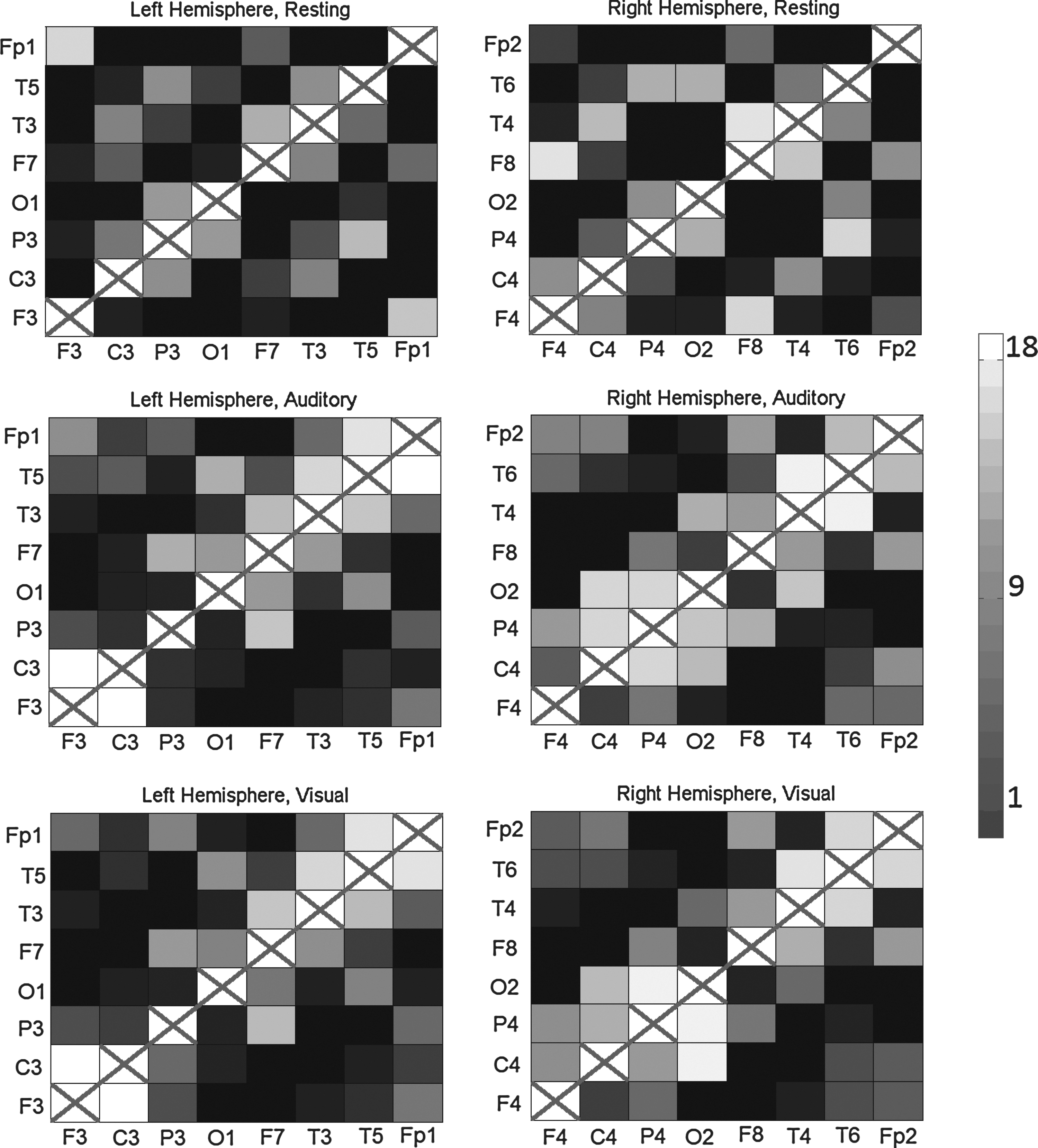
Results of the PSGC analyses between electrode sites in 18 EEG recordings. The i,j cell of the matrix represents the PSGC from region i to region j. The gray scale (see colorbar) represents the number of participants where there is significant connectivity. A black cell means no participants had significant connectivity, whereas a white square signifies information transmission in all 18 participants. Results among left hemisphere locations are on the left, right hemisphere locations on the right. The three rows correspond to resting (top), auditory (middle), and visual (bottom).

Sample connectivity maps from two participants can be seen in Figure 9 (connectivity maps for all participants can be found in Supplementary Section S3). In the resting condition, the LRT finds many short-range (neighbouring site) connections, whereas both the auditory and visual tasks show more long-range connections. The connections in the vigilance tasks are predominantly anterior–posterior, connecting the prefrontal sites to the parietal sites, instead of lateral–medial. This may reflect engagement of the frontal and posterior attention systems in the two vigilance tasks (Wang et al., 2009). Taken with the results of the simulation study, the short-range connections in the resting task may be a result of volume conduction; however, the long-range connections in the active tasks would not be observed without some underlying frontal–posterior coupling. The connectivity matrices do not show any obvious group level asymmetries (consistent with the net GC analysis); however, looking at individual networks suggests that asymmetries may exist, but are not consistent across participants due to individual differences.

FIG. 9.

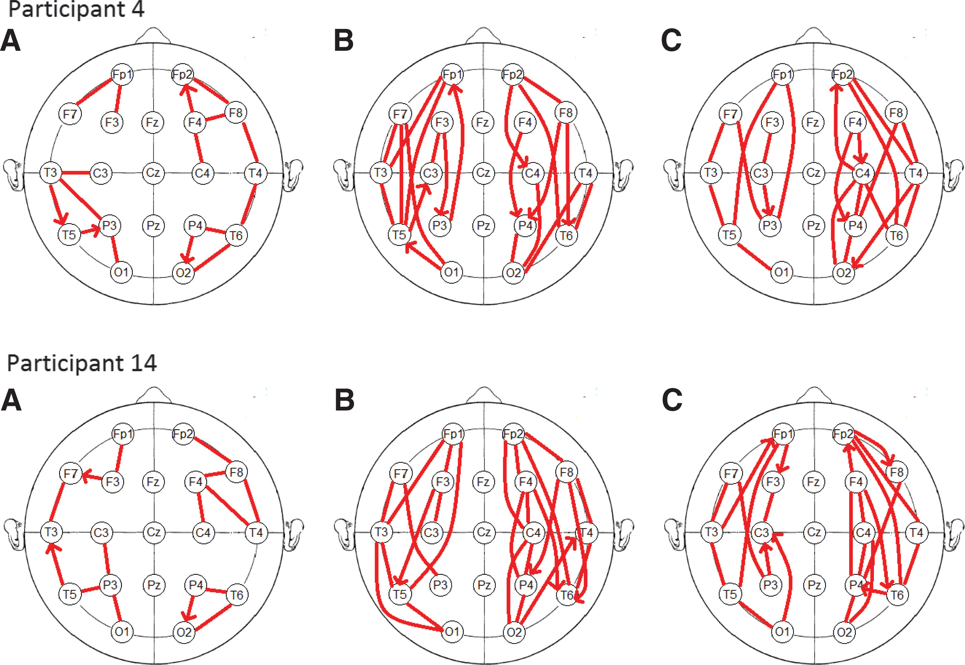
Maps of the estimated network connectivity during the (A) resting, (B) auditory, and (C) visual tasks, for the \documentclass{aastex}\usepackage{amsbsy}\usepackage{amsfonts}\usepackage{amssymb}\usepackage{bm}\usepackage{mathrsfs}\usepackage{pifont}\usepackage{stmaryrd}\usepackage{textcomp}\usepackage{portland, xspace}\usepackage{amsmath, amsxtra}\pagestyle{empty}\DeclareMathSizes{10}{9}{7}{6}\begin{document}$$\chi^{2}$$\end{document} analysis of two individual participants. In the resting task they see many short-range connections, but relatively few long-range connections. In contrast, the active tasks show many connections over longer distances, primarily anterior–posterior, connecting prefrontal sites to parietal sites. Asymmetries are observed in these individual networks; however, the direction is not consistent between individuals. This pattern was consistent across all participants and is further quantified in Figure 10. Color images available online at www.liebertpub.com/brain

Group effects

In addition to looking for connectivity at the individual level, they also analyzed network patterns across the entire group. To identify connections which were active across many participants, the net GC analysis was used to identify connectivity at the group level. The net GC analysis identified only two significant asymmetries at the group level, a short-range prefrontal connection in the resting task ( \documentclass{aastex}\usepackage{amsbsy}\usepackage{amsfonts}\usepackage{amssymb}\usepackage{bm}\usepackage{mathrsfs}\usepackage{pifont}\usepackage{stmaryrd}\usepackage{textcomp}\usepackage{portland, xspace}\usepackage{amsmath, amsxtra}\pagestyle{empty}\DeclareMathSizes{10}{9}{7}{6}\begin{document}$$F7 \rightarrow F3$$\end{document} ) and a connection leaving the visual cortex \documentclass{aastex}\usepackage{amsbsy}\usepackage{amsfonts}\usepackage{amssymb}\usepackage{bm}\usepackage{mathrsfs}\usepackage{pifont}\usepackage{stmaryrd}\usepackage{textcomp}\usepackage{portland, xspace}\usepackage{amsmath, amsxtra}\pagestyle{empty}\DeclareMathSizes{10}{9}{7}{6}\begin{document}$$( O2 \rightarrow C4 )$$\end{document} in the visual condition. The lack of asymmetric connectivity at the group level suggests that the results at the individual level are a result of a feedback relationship between the frontal and posterior regions during the active tasks, or that there are individual differences in the asymmetries observed from the recording.

Network effects

Individual networks were additionally quantified using the network average of local clustering coefficients, a graph theoretical measure which has been used in describing small-world networks in functional connectivity (Sporns and Zwi, 2004; Watts and Strogatz, 1998). The local clustering coefficient measures the degree to which neighbors of a node are interconnected. The average clustering coefficients were used as the dependent variable in a 2 (hemispheres) ×3 (conditions) repeated measures ANOVA, with p-value corrections for sphericity using Greenhouse-Geisser. The resting task (M=0.114, SE=0.028) had significantly lower clustering coefficients than the auditory (M=0.243, SE=0.047) and visual tasks (M=0.196, SE=0.031), F(2, 34)=5.213, p=0.022.

The authors performed a further test of the reliability of the PSGC effects by examining the directed connectivity patterns as a function of the three conditions across participants. To follow up on the descriptive findings outlined above, they focused on short versus long connections. The number of significant directed connections per person was the dependent variable in a 2 (hemispheres) ×3 (conditions) ×2 (connection lengths) within-subject analysis of variance, with p-value corrections for sphericity using Greenhouse-Geisser. The right hemisphere sites (M=8.417, SE=0.381) demonstrated significantly more overall connections than the left (M=7.176, SE=0.384), F(1, 17)=12.374, p=0.003. Similarly, the vigilance tasks elicited more connections (M=8.958, SE=0.684 and M=8.347, SE=0.381 for the auditory and visual tasks, respectively) than did the resting condition (M=6.083, SE=0.349), F(2, 34)=14.308, p<0.001. There were significantly more short (M=9.139, SE=0.431) than long (M=6.4537, SE=0.394) connections, F(1, 17)=55.63, p<0.001. There was a Hemisphere x Connection Length interaction, F(1, 17)=8.011, p=0.012; both hemispheres showed similar amounts of long connections, but the right hemisphere had more short-range connections (M=8.037, SE=0.403) than the left hemisphere (M=10.241, SE=0.551). Of particular interest was the Task x Connection Length interaction, which was highly reliable, F(2, 34)=145.5, p<0.0001, with the mean values illustrated in Figure 10. To examine the reliability of this pattern further, they constructed for each participant a metric reflecting the extent to which the resting condition was associated with more short connections than the active tasks and the active tasks more long connections than the resting condition. This yielded totals for the left hemisphere and right hemisphere for each participant. Each hemisphere of every participant followed this general classification (range=0.5–19.5, with any value above zero indicating this general pattern), indicating extremely high reliability of the pattern illustrated in Figure 10.

FIG. 10.

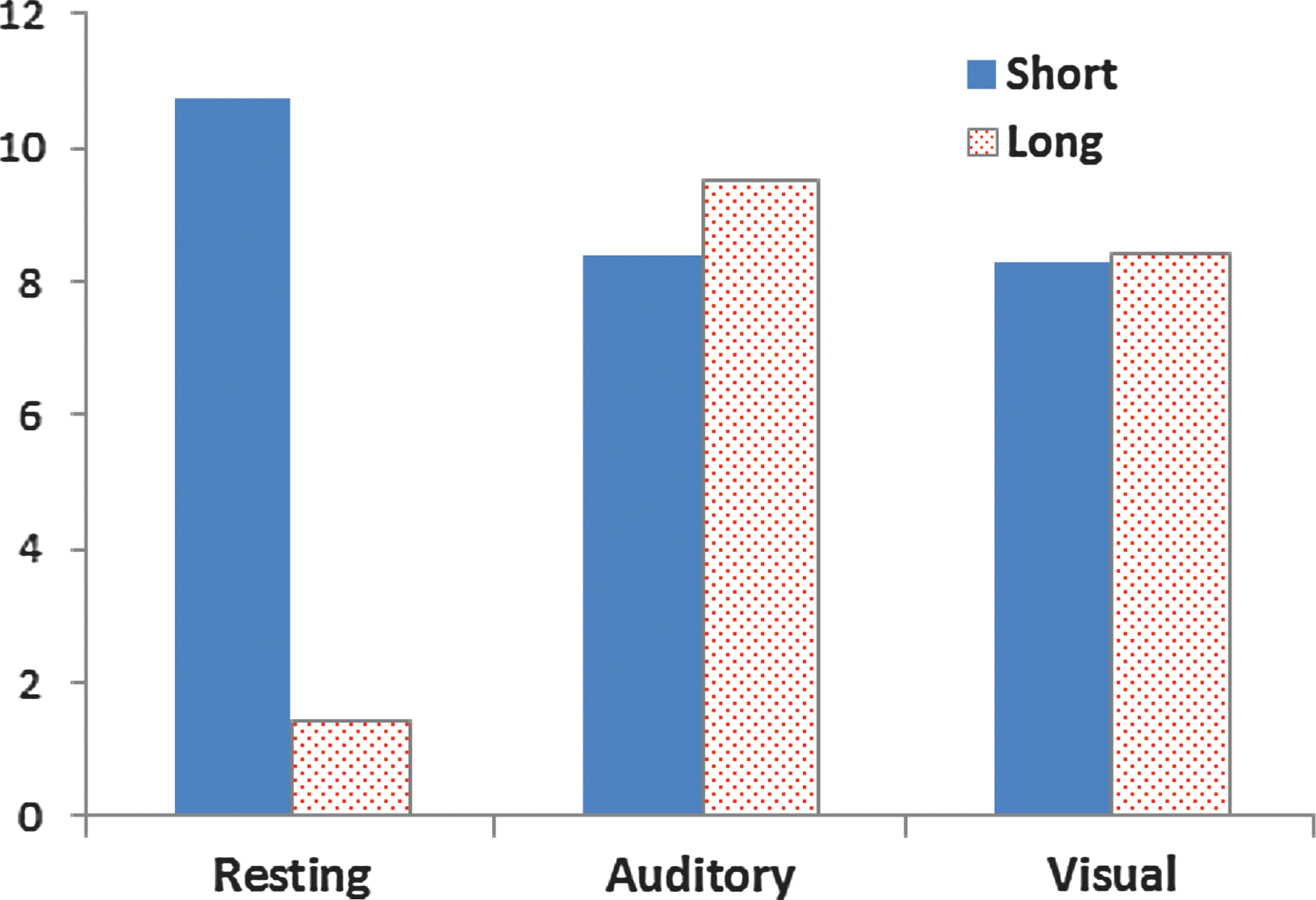
The significant Task×Connection Length interaction, demonstrating an increase in longer connections and a reduction in shorter connections during the auditory and visual vigilance tasks compared with the resting condition. Color images available online at www.liebertpub.com/brain

Alternative explanations

To eliminate the possibility that the observed task connectivity pattern differences were a result of differences in the rate of phase shift events, rather than actual connectivity between regions, they investigated the rate of shift events for each task. The average (standard deviation) rate of phase shift events, across all channels and all participants was 1.16 (0.11) shifts per second during the resting task, 1.12 (0.11) shifts per second in the auditory task, and 1.17 (0.06) shifts per second during the visual task. Another feature of the distribution of phase shift events which explains the lower standard deviation of the visual task is that the resting and auditory tasks both showed heavy left tails, that is, channels with low rates of shift events (as low as 0.8 per sec), whereas the visual task did not (all channels above 1.0 per sec). Since the rate of shift events for the resting task was between the rates for the auditory and visual tasks, and the visual condition had less variability in shift rate than both the auditory and resting tasks, the distribution of shifting rates could not account for the observed connectivity differences between vigilance and resting tasks.

As expected, the resting condition elicited greater alpha amplitude than did the vigilance conditions (which did not differ), whether calculated in terms of absolute alpha amplitude across all sites, relative amplitude (i.e., as a percentage of total amplitude), and whether the ANOVA is run with all eight sites (i.e., site factor with eight levels) as levels of the independent variable or with them summed into the four more frontocentral versus four posterior sites (site with two levels; all p<0.001). There were also various effects of left versus right, and anterior versus posterior sites, and their interactions, but these are not related to their primary focus. However, important for their analysis, alpha power values did not correlate with rates of phase shift events (r=0.05, p=0.13).

Additionally, the authors estimated the PDC value for each recording to determine if the results of the PSGC analysis were providing additional insight into the data beyond what could be found with traditional methods. A 10th order multivariate AR model was estimated for the eight within hemisphere channels in each hemisphere and each recording to calculate the PDC values (Schelter et al., 2005). The resulting PDC values were compared with the corresponding PSGC values using a nonparametric Spearman's rho correlation. The results showed no significant correlation between the PDC and PSGC values for the resting (r=0.009), auditory (r=−0.032), or visual tasks (r=−0.039). Although the signs of the estimated correlation are different for the resting and vigilance tasks, the magnitude of the correlations is too small to represent a meaningful relationship.

Discussion

This article demonstrates a novel method for analyzing neural connectivity from EEG recordings. The PSGC measure is a phase-based method which identifies spontaneous desynchronizations called phase shifts, and then models the events as a full multivariate point process. By applying the ideas of Granger causality, an asymmetric measure is produced which takes into account the effect of all other signals and can be used to infer directed connectivity between neural regions. Using instantaneous phase, the PSGC measure is able to take advantage of the full temporal resolution of the EEG recording and capture nonlinear relationships which are not detectable by traditional coherence. Measures of coherence quantify the strength and consistency of phase relationships, but when there is desynchronization within the signal it does not provide any information about this desynchrony. The PSGC measure explores a different aspect of functional integration (see Alternative explanations section) by exploring the nature of desynchronization, and elucidating spatiotemporal patterns of phase shift events. They have presented two different statistical techniques for analyzing the results of PSGC, a LRT for Granger causality in individual networks, which uses a \documentclass{aastex}\usepackage{amsbsy}\usepackage{amsfonts}\usepackage{amssymb}\usepackage{bm}\usepackage{mathrsfs}\usepackage{pifont}\usepackage{stmaryrd}\usepackage{textcomp}\usepackage{portland, xspace}\usepackage{amsmath, amsxtra}\pagestyle{empty}\DeclareMathSizes{10}{9}{7}{6}\begin{document}$$\chi^{2}$$\end{document} distribution (see Equation 23), and a group level t-test for net Granger causality (see Equation 25), which uses time-reversed surrogate data (Haufe et al., 2013). The net GC analysis is the preferred test for identifying asymmetric connectivity at the group level; it is designed to maximize the statistical power to identify asymmetries and the results of the simulation study suggest that it is not affected by volume conduction. The method identifies the true asymmetric connection ( \documentclass{aastex}\usepackage{amsbsy}\usepackage{amsfonts}\usepackage{amssymb}\usepackage{bm}\usepackage{mathrsfs}\usepackage{pifont}\usepackage{stmaryrd}\usepackage{textcomp}\usepackage{portland, xspace}\usepackage{amsmath, amsxtra}\pagestyle{empty}\DeclareMathSizes{10}{9}{7}{6}\begin{document}$$F4 \rightarrow O2$$\end{document} ) for each of the noise conditions, but is unable to quantify the feedback connection. The \documentclass{aastex}\usepackage{amsbsy}\usepackage{amsfonts}\usepackage{amssymb}\usepackage{bm}\usepackage{mathrsfs}\usepackage{pifont}\usepackage{stmaryrd}\usepackage{textcomp}\usepackage{portland, xspace}\usepackage{amsmath, amsxtra}\pagestyle{empty}\DeclareMathSizes{10}{9}{7}{6}\begin{document}$$\chi^{2}$$\end{document} analysis is also able to identify asymmetric connections; however, it also identifies bidirectional connections making it appropriate when the goal is to analyze network patterns as a whole. Another benefit of the \documentclass{aastex}\usepackage{amsbsy}\usepackage{amsfonts}\usepackage{amssymb}\usepackage{bm}\usepackage{mathrsfs}\usepackage{pifont}\usepackage{stmaryrd}\usepackage{textcomp}\usepackage{portland, xspace}\usepackage{amsmath, amsxtra}\pagestyle{empty}\DeclareMathSizes{10}{9}{7}{6}\begin{document}$$\chi^{2}$$\end{document} analysis is that it can be applied directly to individuals to analyze individual differences in network connectivity, whereas the net GC analysis is restricted to group results which assume commonality of a specific directed connection across individuals. Given the multiple processes involved in all experimental tasks and the mixture of signals at the scalp, they do not expect group commonality as reliably as they see individual effects.

In the simulation study, it was confirmed that the PSGC measure is able to correctly identify the direction of information transfer in conditions similar to those of EEG recordings. The simulated data contain multiple sources of noise, both independent additive noise and spatiotemporal sources of biological noise. The simulation showed that the existence of spatiotemporal noise helped to attenuate the spread of phase shift events due to volume conduction or average reference. The \documentclass{aastex}\usepackage{amsbsy}\usepackage{amsfonts}\usepackage{amssymb}\usepackage{bm}\usepackage{mathrsfs}\usepackage{pifont}\usepackage{stmaryrd}\usepackage{textcomp}\usepackage{portland, xspace}\usepackage{amsmath, amsxtra}\pagestyle{empty}\DeclareMathSizes{10}{9}{7}{6}\begin{document}$$\chi^{2}$$\end{document} analysis on individual networks did not show spurious connectivity when the bSNR levels were below −2.7 dB, but larger bSNRs showed spread of connectivity across several electrodes. The ability to identify connectivity in scenarios with very low bSNR is a strength of the PSGC measure; the high levels of noise that are typical in continuous EEG recordings actually help reduce the extent to which volume conduction produces spurious connectivity measurements.

The existence of high levels of noise is one of the main challenges in EEG analysis. The most popular method of dealing with this noise is to average time-locked waveforms from many trials, under the assumption that unrelated background activity will decrease as the number of trials goes up; however, evidence suggests that phase information contained in the background activity is important to understanding brain activity (Makeig et al., 2002). This emphasizes the need for measures like PSGC which can be used in low bSNR conditions to analyze nonaveraged EEG recordings.

For this proof-of-concept study, the estimated connectivity networks are evaluated by predictions based on the role of attention in vigilance tasks; however, the estimated networks should not be taken as a complete description of attention networks. The primary result of interest supports the prediction concerning connectivity during complex attention versus a resting state: the number of significant short connections during the resting state exceeds those during the vigilance tasks, but of more importance, the longer distance connections dramatically increase during the vigilance tasks. This is consistent with the expected connectivity given the neurophysiology of attention (Berger et al., 2007; Buschman and Miller, 2007; Rueda et al., 2005; Silton et al., 2010). There were, in addition, some main effects that also confirmed expectations. The active tasks had significantly higher clustering coefficients than the resting task, a feature associated with small-world networks (Sporns et al., 2004). Similarly, there was an increase (albeit minor) in overall connectivity during the active tasks. The finding of more significant instances of connectivity for the short (across adjacent sites) compared with the long (across more distant sites) may be due to passive transmission being greater over short distances, and is only of interest when interacting with task requirements, as was found in their study, with this pattern present for every participant. Converging evidence from these measures of network connectivity strongly suggest differing patterns of neural connectivity between resting and active tasks.

Volume conduction, reference electrode, and stationarity

When analyzing a mixture of signals, the overall phase is an amplitude weighted function of the phase of the individual components. This means that the phase of the dominant component is most represented in the signal. When identifying phase shift events, contributions from weaker components of the signal may not have a large enough effect on the overall phase to reach the threshold value. The use of a well-chosen threshold value can effectively eliminate phase shifts from weak contributions, such as those due to volume conduction over large distances (strength of volume conduction decreases quadratically with distance). This result is confirmed by the simulation study, where low bSNRs ( \documentclass{aastex}\usepackage{amsbsy}\usepackage{amsfonts}\usepackage{amssymb}\usepackage{bm}\usepackage{mathrsfs}\usepackage{pifont}\usepackage{stmaryrd}\usepackage{textcomp}\usepackage{portland, xspace}\usepackage{amsmath, amsxtra}\pagestyle{empty}\DeclareMathSizes{10}{9}{7}{6}\begin{document}$$\le$$\end{document} −2.7 dB) showed minimal effects of volume conduction, whereas the high bSNR (>− 2.7 dB) showed high rates of observed connectivity due to volume conduction. Further evidence for this result is shown in Supplementary Sections S1 and S2, where they quantify the effects of noise, volume conduction and reference electrode on the identification of phase shift events.

Another consideration for use in EEG recordings is the effect of reference choice on the phase of a signal. Using an average reference can cause inflated connectivity in measures such as coherence (Nunez et al., 1997; Rappelsberger, 1989), and can cause phase variables to lose physiological importance (Thatcher, 2010). The authors argue that the latter is not the case when measuring PSGC, because it analyzes qualitative features of the signal (phase shifts modeled as a point process) rather than interpreting the magnitude of the phase variables directly. Additionally, because each signal contributes only a small amount to the average (1/121 in the real recordings), with realistic amounts of biological activity, the phase shifts in the reference will be strongly attenuated and, therefore, will be eliminated by the threshold technique. They do not expect the average reference to contribute to network connectivity.

Calculating the bSNR from EEG recordings requires the use of an inverse method to identify the different biological components, making estimates of the bSNR highly dependent on the specific inverse method used. To get an idea of the bSNR that can be expected in nonaveraged EEG data, they can use results from independent component analysis (ICA). In Delorme and associates (2012), twenty different ICA algorithms are each applied to EEG recordings from a visual attention task; they found an average of 22.4 dipole-like biological components (range 9.1–37.4). The strengths of the individual components are not reported, but these authors can infer an average component strength of 4.5% (range 2.6–11%). This is well below the 35/2=17.5% per component level where volume conduction and reference electrode became a concern in the simulations. A bSNR of greater than −2.7 dB is not realistic for nonaveraged EEG recordings, which are notorious for having large amounts of noise, so they conclude that observed connectivity difference between resting and vigilance tasks are not due to volume conduction or reference electrode.

Stationarity is a concern when modeling long (more than several seconds) EEG recordings as an AR process (Cohen and Sances, 1977; Ding et al., 2000; Wang et al., 2008). The PSGC analysis presented in this study uses a highly nonlinear transformation from a time series to a point process and the aforementioned results based on linear AR models are not directly applicable. To the best of their knowledge, this is the first attempt to model EEG recordings in this manner and there are no existing results on the stationarity (or nonstationarity) of such a process. In this study, the authors have applied the PSGC analysis to continuous EEG recordings of up to 15 min in length. This is justified by a preliminary stationarity analysis using the two sample Kolmogorov–Smirnov test, described in Supplementary Section S4, which found no evidence of nonstationarity. This means that any spontaneous phase shift events which occur unrelated to the task at hand do not have consistent spatiotemporal patterns and are viewed as residuals of the model. It would also be possible to apply the PSGC method to shorter length segments of data; however, each segment would require at least M x W points of data to establish initial conditions for the method.

Future work

It is possible to extend this work by including additional information into the history H_t of the model CIF, for example, by including the stimulus onset times into the model. In this study they have restricted their analysis to the 8–10 Hz frequency band, but it would be possible to perform the analysis on other bands or to include multiple bands and allow for inter-band connectivity.

A natural extension of the PSGC method is to evolve it to work on the results of an ICA (or other source reconstruction technique), although this may limit applicability due to increased technical requirements, or when working with special populations where adequate data are not available. In these situations it is beneficial to have a method which can be directly applied to EEG scalp recordings. Proceeding in this manner should be done with caution, as at this time it is not clear whether such inverse solutions are able to properly maintain phase relations.

Footnotes

Acknowledgments

The authors would like to thank James Desjardins for his insights regarding the application of PSGC to EEG recordings. This work has been funded by the Natural Sciences and Engineering Research Council of Canada (NSERC) for doctoral support to WJM and CLL; the data collection was supported by operating grants from the Canadian Institutes for Health Research (CIHR) and NSERC to SJS.

Author Disclosure Statement

No competing financial interests exist.

References

Akaike

. 1974. A new look at the statistical model identification. IEEE Trans Autom Control, 19:716–723.

Astolfi

, Cincotti

, Mattia

, Fallani

FDV

, Tocci

, Colosimo

, Salinari

, Marciani

, Hesse

, Witte

, Ursino

, Zavaglia

, Babiloni

. 2008. Tracking the time-varying cortical connectivity patterns by adaptive multivariate estimators. IEEE Trans Biomed Eng, 55:902–913.

Astolfi

, Toppi

, Fallani

FDV

, Vecchiato

, Salinari

, Mattia

, Cincotti

, Babiloni

. 2010. Neuroelectrical hyperscanning measures simultaneous brain activity in humans. Brain Topogr, 23:243–356.

Atkinson

. 1989. An Introduction to Numerical Analysis. John Wiley & Sons.

Baccala

, Sameshima

. 2001. Partial directed coherence: a new concept in neural structure determination. Biol Cybern, 84:463–474.

Barabasi

A-L

, Albert

. 1999. Emergence of scaling in random networks. Science, 286:509–512.

Berger

, Kofman

, Livneh

, Henik

. 2007. Multidisciplinary perspectives on attention and the development of self-regulation. Prog Neurobiol, 82:256–286.

Bingham

, Godfrey

, Tukey

. 1967. Modern techniques of power spectrum estimation. IEEE Trans on Audio and Electroacoustics, AU-15:56–66.

Boccaletti

, Kurths

, Osipov

, Valladares

, Zhou

. 2002. The synchronization of chaotic systems. Phys Rep, 366:1–101.

10.

Braitenberg

. 1985. Charting the visual cortex. Cerebral Cortex, 3:379–414.

11.

Breakspear

, Williams

, Stam

. 2004. A novel method for the topographic analysis of neural activity reveals formation and dissolution of `dynamic cell assemblies'. J Comp Neurol, 16:49–68.

12.

Bressler

, Coppola

, Nakamura

. 1993. Episodic multiregion cortical coherence at multiple frequencies during visual task performance. Nature, 366:153–156.

13.

Buschman

, Miller

. 2007. Top-down versus bottom-up control of attention in the prefrontal and posterior parietal cortices. Science, 315:1860–1862.

14.

ten Caat

, Lorist

, Bezdan

, Roerdink

, Maurits

. 2008. High density EEG coherence analysis using functional units applied to mental fatigue. J Neurosci Methods, 171:271–278.

15.

Calvert

, Hansen

, Iversen

, Brammer

. 2001. Detection of audio-visual integration sites in humans by applications of electrophysiological criteria to the bold effect. NeuroImage, 14:427–438.

16.

Chavez

, Besserve

, Adam

, Martinerie

. 2006. Towards a proper estimation of phase sychronization from time series. J Neurosci Methods, 154:149–160.

17.

Cimponeriu

, Rosenblum

, Fieseler

, Dammers

, Schiek

, Majtanik

, Morosan

, Bezerianos

, Tass

. 2003. Inferring asymmetric relations between interacting neural oscillators. Prog Theor Phys Suppl, 150:22–36.

18.

Cohen

, Sances

. 1977. Stationarity of the human electroencephalogram. Med Biol Eng Comput, 15:513–518.

19.

Daley

, Vere-Jones

. 2003. An Introduction to the Theory of Point Processes. Springer.

20.

Delorme

, Makeig

. 2004. EEGLAB: an open source toolbox for analysis of single-trial EEG dynamics including independent component analysis. J Neurosci Methods, 134:9–21.

21.

Delorme

, Palmer

, Onton

, Oostenveld

, Makeig

. 2012. Independent EEG sources are dipolar. PLoS One, 7:e30135.

22.

Ding

, Bressler

, Yang

, Liang

. 2000. Short-window spectral analysis of cortical event-related potentials by adaptive multivariate autoregressive modeling: Data preprocessing, model validation, and variability assessment. Biol Cybern, 83:35–45.

23.

Eriksen

, Eriksen

. 1974. Effects of noise letters upon the identification of a target letter in a nonsearch task. Percept Psychophys, 16:143–149.

24.

Finkel

, Edelman

. 1989. Integration of distributed cortical systems by reentry: A computer simulation of interactive functionally segregated visual areas. J Neurosci, 9:3188–3208.

25.

Friston

. 1994. Functional and effective connectivity in neuroimaging: a synthesis. Hum Brain Mapp, 2:56–78.

26.

Gabor

. 1946. Theory of communication. J Inst Electr Eng, 93:429–457.

27.

Goodman

. 1960. Measuring amplitude and phase. J Franklin Inst, 270:437–450.

28.

Granger

. 1969. Investigating causal relations by econometric models and cross-spectral methods. Econometrica, 37:424–438.

29.

Gratton

, Coles

, Donchin

. 1983. A new method for off-line removal of ocular artifact. Electroencephalogr Clin Neurophysiol, 55:468–484.

30.

Gray

. 1999. The temporal correlation hypothesis of visual feature integration: still alive and well. Neuron, 24:31–47.

31.

Haufe

, Nikulin

, Muller

K-R

, Nolte

. 2013. A critical assessment of connectivity measures for EEG data: a simulation study. NeuroImage, 64:120–133.

32.

Hesse

, Moller

, Arnold

, Schack

. 2003. The use of time-variant EEG granger causality for inspecting directed interdependencies of neural assemblies. J Neurosci Methods, 124:27–44.

33.

Holm

. 1979. A simple sequentially rejected multiple test procedure. Scand J Statist, 6:65–70.

34.

Jasper

. 1958. Report on the committee on methods of clinical examination in electroencephalography. Electroencephalogr Clin Neurophysiol, 10:370–375.

35.

John

. 2005. From synchronous neural discharges to subjective awareness? In: Laureys

(ed.) Progress in Brain Research, Chapter 11. Elsevier B.V. volume 150.

36.

Kiemel

, Gormley

, Guan

, Williams

, Cohen

. 2003. Estimating strength and direction of functional coupling in the lamprey spinal cord. J Comput Neurosci, 15:233–245.

37.

Kim

, Putrino

, Ghosh

, Brown

. 2011. A granger causality measure for point process models of ensemble neural spiking activity. PLoS Comput Biol, 7:1–13.

38.

Koeda

, Knyazeva

, Njiokiktjien

, Jonkman

, Sonneville

, Vildavsky

. 1995. The EEG in acallosal children. coherence values in the resting state: Left hemisphere compensatory mechanism. Electroencephalogr Clin Neurophysiol, 95:397–407.

39.

Lackner

, Marshall

, Santesso

, Dywan

, Wade

, Segalowitz

. 2014. Adolescent anxiety and aggression can be differentially predicted by electrocortical phase reset variables. Brain Cognition, 89:90–98.

40.

Liao

, Zhang

, Pan

, Mantini

, Ding

, Duan

, Luo

, Lu

, Chen

. 2010. Altered functional connectivity and small-world in mesial temporal lobe epilepsy. PLoS One, 5:e8525.

41.

Liu

, Liang

, Zhou

, He

, Hao

, Song

, Yu

, Liu

, Jiang

. 2008. Disrupted small-world networks in schizophrenia. Brain, 131:945–961.

42.

Llinás

, Ribary

. 1998. Temporal conjunction in thalamocortical transactions. In: Jasper

, Descarries

, Castellucci

, Rossignol

(eds.) Consciousness: At the Frontiers of Neuroscience, Advances in Neurology. Philadelphia: Lippincotti-Raven Publishers; volume 77.

43.

Lobier

, Siebenhühner

, Palva

. 2014. Phase transfer entropy: A novel phase-based measure for directed connectivity in networks coupled by oscillatory interactions. NeuroImage, 85:853–872.

44.

Makeig

, Westerfield

, Jung

T-P

, Enghoff

, Townsend

, Courchesne

, Sejnowski

. 2002. Dynamic brain sources of visual evoked responses. Science, 295:690–694.

45.

Moller

, Schack

, Arnold

, Witte

. 2001. Instantaneous multivariate EEG coherence analysis by means of adaptive high-dimensional auto-regressive models. J Neurosci Methods, 105:143–158.

46.

Mosher

, Leahy

, Lewis

. 1999. EEG and MEG: Forward solutions for inverse problems. IEEE Trans Biomed Eng, 46:245–259.

47.

Murias

, Webb

, Greenson

, Dawson

. 2007. Resting state cortical connectivity reflected in EEG coherence in individuals with autism. Biol Psychiatry, 62:270–273.

48.

Nolte

, Bai

, Wheaton

, Mari

, Vorbach

, Hallett

. 2004. Identifying true brain interaction from EEG data using the imaginary part of coherency. Clin Neurophysiol, 115:2292–2307.

49.

Nolte

, Ziehe

, Nikulin

, Schlogl

, Kramer

, Brismar

, Muller

K-R

. 2008. Robustly estimating the flow direction of information in complex physical systems. Phys Rev Lett, 100:234101.

50.

Nunez

, Srinivasan

, Westdorp

, Wijesinghe

, Tucker

, Silberstein

, Cadusch

. 1997. EEG coherency I: Statistics, reference electrode, volume conduction, laplacians, cortical imaging, and interpretation at multiple scales. Electroencephalogr Clin Neurophysiol, 103:499–515.

51.

Pikovsky

, Rosenblum

, Knuths

. 2003. Synchronization: A Universal Concept in Nonlinear Sciences. New York: Cambridge Univ Press.

52.

Pikovsky

, Rosenblum

, Osipov

, Kurths

. 1997. Phase synchronization of chaotic oscillators by external driving. Physica D, 104:219–238.

53.

Quyen

MLV

, Foucher

, Lachaux

J-P

, Rodriguez

, Lutz

, Martinerie

, Varela

. 2001. Comparison of Hilbert transform and wavelet methods for the analysis of neural synchrony. J Neurosci Methods, 111:83–98.

54.

Rappelsberger

. 1989. The reference problem and mapping of coherence: a simulation study. Brain Topography, 2:63–72.

55.

Rosenblum

, Cimponeriu

, Bezerianos

, Patzak

, Mrowka

. 2002. Identification of coupling direction: application to cardiorespiratory interaction. Phys Rev E, 65:041909.

56.

Rosenblum

, Pikovsky

. 2001. Detecting direction of coupling in interacting oscillators. Phys Rev E, 64:045202.

57.

Rueda

, Posner

, Rothbart

. 2005. The development of executive attention: Contributions to the emergence of self-regulation. Dev Neuropsychol, 28:573–594.

58.

Saito

, Harashima

. 1981. Tracking information within multichannel EEG record: Causal analysis in EEG. In: Yamaguchi

, Fujisawa

(eds.) Recent Advances in EEG and MEG Data Processing; pp. 133–146.

59.

Schelter

, Winterhalder

, Eichler

, Peifer

, Hellwig

, Guschlbauer

, Lucking

, Dahlhaus

, Timmer

. 2005. Testing for directed influences among neural signals using partial directed coherence. J Neurosci Methods, 152:210–219.

60.

Silton

, Heller

, Towers

, Engels

, Spielberg

, Edgar

, Sass

, Stewart

, Sutton

, Banich

, Miller

. 2010. The time course of activity in dorsolateral prefrontal cortex and anterior cingulate cortex during top-down attention control. NeuroImage, 50:1292–1302.

61.

Smirnov

, Bezruchko

. 2003. Estimation of interaction strength and direction from short and noisy time series. Phys Rev E, 68:046209.

62.

Sporns

, Chialvo

, Kaiser

, Hilgetag

. 2004. Organization, development and function of complex brain networks. TRENDS Cogn Sci, 8:418–425.

63.

Sporns

, Tononi

, Edelman

. 1991. Modeling perceptual grouping and figure ground segregation by means of active reentry connections. Proc Natl Acad Sci U S A, 88:129–133.

64.

Sporns

, Tononi

, Edelman

. 2000. Theoretical neuroanatomy: Relating anatomical and functional connectivity in graphs and cortical connection matrices. Cereb Cortex, 10:127–141.

65.

Sporns

, Zwi

. 2004. The small world of the cerebral cortex. Neuroinformatics, 2:145–162.

66.

Steriade

. 1995. Cellular substrates of brain rhythms. In: Niedermeyer

, da Silva

(eds.) Electroencephalography. Baltimore: Williams and Wilkins.

67.

Takahashi

, Baccala

, Sameshime

. 2007. Connectivity inference between neural structures via partial directed coherence. J Appl Stat, 34:1255–1269.

68.

Tass

, Rosenblum

, Weule

, Kurths

, Pikovsky

, Volkmann

, Schnitzler

, Freund

. 1998. Detection of n:m phase locking from noisy data: application to magnetoencephalography. Phys Rev Lett, 81:3291–3294.

69.

Thatcher

. 1992. Cyclic cortical reorganization during early childhood. Brain Cogn, 20:24–50.

70.

Thatcher

. 2010. Coherence, phase differences, phase shift and phase lock in EEG/ERP analysis. Dev Neuropsych, 37:476–496.

71.

Thatcher

, Krause

, Hrybyk

. 1986. Cortico-cortical associations and EEG coherence: A two-compartmental model. Electroencephalogr Clin Neurophysiol, 64:123–143.

72.

Thatcher

, North

, Biver

. 2005. EEG and intelligence: univariate and multivariate comparisons between EEG coherence, EEG phase delay and power. Clin Neurophysiol, 116:2129–2141.

73.

Thatcher

, North

, Biver

. 2009. Self-organized criticality and the development of EEG phase reset. Hum Brain Mapp, 30:553–574.

74.

Tononi

, Sporns

, Edelman

. 1992. Reentry and the problem of integrating multiple cortical areas: simulation of dynamic integration in the visual system. Cereb Cortex, 2:310–355.

75.

Tononi

, Sporns

, Edelman

. 1994. A measure for brain complexity: Relating functional segregation and integration in the nervous system. Proc Natl Acad Sci U S A, 91:5033–5037.

76.

Vakorin

, Mišić

, Krakovska

, Bezgin

, McIntosh

. 2013. Confouding effects of phase delays on causality estimation. PLoS One, 8:e53588.

77.

Varela

, Lachaux

J-P

, Rodriguez

, Martinerie

. 2001. The brainweb: phase synchronization and large-scale integration. Nat Rev Neurosci, 2:229–239.

78.

Wang

, Liu

, Guise

, Knight

, Ghajar

, Fan

. 2009. Effective connectivity of the fronto-parietal network during attentional control. J Cogn Neurosci, 22:543–553.

79.

Wang

, Chen

, Ding

. 2008. Estimating granger causality after stimulus onset: a cautionary note. Neuroimage, 41:767–776.

80.

Watts

, Strogatz

. 1998. Collective dynamics of ‘small-world’ networks. Nature, 393:440–442.

Supplementary Material

Please find the following supplemental material available below.

For Open Access articles published under a Creative Commons License, all supplemental material carries the same license as the article it is associated with.

For non-Open Access articles published, all supplemental material carries a non-exclusive license, and permission requests for re-use of supplemental material or any part of supplemental material shall be sent directly to the copyright owner as specified in the copyright notice associated with the article.

0.00 MB

0.35 MB