Using the Virtual Brain to Reveal the Role of Oscillations and Plasticity in Shaping Brain's Dynamical Landscape

Abstract

Spontaneous brain activity, that is, activity in the absence of controlled stimulus input or an explicit active task, is topologically organized in multiple functional networks (FNs) maintaining a high degree of coherence. These “resting state networks” are constrained by the underlying anatomical connectivity between brain areas. They are also influenced by the history of task-related activation. The precise rules that link plastic changes and ongoing dynamics of resting-state functional connectivity (rs-FC) remain unclear. Using the framework of the open source neuroinformatics platform “The Virtual Brain,” we identify potential computational mechanisms that alter the dynamical landscape, leading to reconfigurations of FNs. Using a spiking neuron model, we first demonstrate that network activity in the absence of plasticity is characterized by irregular oscillations between low-amplitude asynchronous states and high-amplitude synchronous states. We then demonstrate the capability of spike-timing-dependent plasticity (STDP) combined with intrinsic alpha (8–12 Hz) oscillations to efficiently influence learning. Further, we show how alpha-state-dependent STDP alters the local area dynamics from an irregular to a highly periodic alpha-like state. This is an important finding, as the cortical input from the thalamus is at the rate of alpha. We demonstrate how resulting rhythmic cortical output in this frequency range acts as a neuronal tuner and, hence, leads to synchronization or de-synchronization between brain areas. Finally, we demonstrate that locally restricted structural connectivity changes influence local as well as global dynamics and lead to altered rs-FC.

Introduction

Structure and function

One of the major open questions in neuroscience is the relationship between structure and function. Several spatiotemporal features of resting-state functional connectivity (rs-FC) have been captured by existing modeling approaches (Deco et al., 2011, 2013b). A systematic framework for relating structural connectivity (SC) and functional connectivity (FC) has been recently provided by The Virtual Brain (TVB), a simulation platform of large-scale brain activity (Ritter et al., 2013; Sanz et al., 2013). There is a lack of mechanistic understanding of changes of network states due to learning/plasticity (Sigala et al., 2014). This article explores how to describe learning and plasticity-related changes of FC with biophysically plausible brain models. With learning and plasticity, we refer to training/exposure-related changes of SC at all spatial brain scales and the resulting functional consequences. Computational insights gained due to structural modifications will add to our understanding of the structure-function relationship provided by previous computational studies (Alstott et al., 2009; Cabral et al., 2012a, 2012b). A key ingredient of our model is the structural brain network defined by empirically derived long-range brain connectivity between regions, resulting in biologically plausible conduction delays. We use a subset of cortical regions represented as nodes in the large-scale brain network. The nodes are dynamical units built of highly interconnected excitatory and inhibitory neurons. The interaction between those regions in the network needs to be uncovered to understand the origin of correlated activity fluctuations in the brain during resting-state and task conditions. Here, we evaluate existing modeling approaches and advance them by incorporating state-dependent local plasticity mechanisms. Specifically, we explore how subcortical input to a cortical region shapes the local SC at a microscopic scale. Subsequently, we investigate the interaction with other cortical regions connected via the realistic anatomical connectivity matrix. Using computational and analytical methods, we show how input oscillations in the alpha (8–12 Hz) frequency range along with plasticity parameters (plasticity time constant, input oscillation frequency) critically influence transition from asynchronous to synchronous state in a local neuronal population. Local oscillations, in turn, reshape evolution of covariance on a longer time scale across a subset of anatomically connected cortical regions. We evaluate theoretical scenarios, how brain states in terms of slow power fluctuation of the local field potential's (LFP) alpha frequency band influence local plasticity. Restructuring of cortical node level synaptic weights due to spike-timing-dependent plasticity (STDP) results in learning phases of firing. In other words, the neurons learn to elicit output population spikes at specific phases of input background oscillations. We find that spatiotemporal low frequency fluctuations (<0.1 Hz) of the simulated signal—similar to those observed in blood oxygenation level-dependent (BOLD) functional magnetic resonance imaging (fMRI) signals during rest—are significantly shaped not only by given anatomical connectivity but also by ongoing synaptic plasticity within cortical regions. Combining brain states and plasticity provides a general theoretical framework for alterations of rs-FC, which reflects ongoing network dynamics and, hence, predicts the outcome of behavioral performance.

Plasticity shapes rs-FC

Typical large-scale interactions between brain areas are concerned with neural assemblies that are farther apart in the brain (>1 cm) with transmission delays in the order of 8–10 msec spanning poly-synapses (Varela et al., 2001). Resting-state networks (RSN) arise from coordinated distributed functional clusters. They give rise to coherent neural activity as a signature of large-scale brain operations in the absence of an explicit task or stimuli (Fox and Raichle, 2007; Smith et al., 2009). RSNs resemble both task-related functional networks (FNs) (Biswal et al., 1995; Fox and Raichle, 2007; Vincent et al., 2007) and anatomical networks, that is, regions directly connected via anatomical pathways (Honey et al., 2009). Recent studies have shown that cortical activation can restructure resting-state activity after task performance (Lewis et al., 2009; Riedl et al., 2011; Tambini et al., 2010; Urner et al., 2013; Zhang et al., 2012). Finally, evidence suggests that perceptual learning modifies the large-scale functional covariance between networks engaged in a task (Cole et al., 2012; Lewis et al., 2009). In line with this, only 30 min of repetitive sensory stimulation (RSS) (Freyer et al., 2012a)—a paradigm known to induce neural plasticity and counteracting sensory decline due to neurological trauma or aging (Kalisch et al., 2008, 2010)—leads to significant changes of the time-lagged coherence in resting-state alpha rhythm within sensorimotor cortical areas (Freyer et al., 2012a). While learning alters resting-state activity, this activity also influences the ability to learn. A recent electroencephalography (EEG) study on perceptual learning showed that high resting-state alpha power contralateral to the stimulated finger is predictive for a greater behavioral improvement after RSS at an inter-subject level (Freyer et al., 2013). These findings provide evidence that the resting brain is not a passive sensory-motor analyzer driven by sensory inputs. Rather, it actively generates predictions about forthcoming sensory stimuli by maintaining a structured memory of past activations that finds expression in the ongoing brain states. Here, we explore the effects of the interplay of RSS-induced plasticity and ongoing brain states in the alpha frequency range as a mechanism that could provide explanation for the corresponding change in FC between somatosensory and motor cortex connected via realistic SC.

Computational modeling

To understand the mechanisms underlying the complex interaction at the neuronal population level during rest and under task-based conditions, brain imaging as well as computational models play complementary roles. Brain imaging monitors cognitive states in the whole brain network at a macroscopic scale. For example, in fMRI, a cortical voxel describes the population activity of a few million neurons. Computational models provide potential underlying mechanisms of interaction between neuronal populations that give rise to the observed spatiotemporal dynamics of BOLD or EEG activity. This is realized by representing functional clusters of neurons by mean field or neural mass models. Mean field or neural mass models attempt to model the dynamics of large (theoretically infinite) populations of neurons. Numerous recent resting-state modeling studies (Cabral et al., 2011; Deco et al., 2013a, 2013c) successfully reconstructed empirically observed RSNs between clusters, patterns of positive and negative correlations as described in many experimental studies by looking at the interplay between local network dynamics and large-scale structure of the brain. In principle, global FC can be altered within milliseconds by perturbation, while the large-scale SC matrix remains fixed or under natural conditions changes only over longer time periods through plasticity processes. However, on a microscopic scale, synaptic dynamics and connectivity are altered within milliseconds (Caporale and Dan, 2008). Emergent FC depends on the dynamics of individual nodes, which are shaped by the local and global neuronal context. In the framework of TVB, this is accounted for by allowing for inputs from multiple connected regions to individual sub-cortical or cortical regions. Key signatures of emergent network dynamics are neuronal oscillations that can be detected by non-invasive brain imaging methods such as EEG.

Overview of the study

In the first section, we discuss ongoing activity at rest and underlying dynamics using two types of models: a spiking model (Deco and Jirsa, 2012), a mean field firing rate model derived from the spiking model (Deco and Jirsa, 2012; Deco et al., 2014). All are capable of generating a similar bifurcation structure. The dynamic mean field (DMF) model and the spiking model are capable of generating a similar bifurcation structure as shown qualitatively in Figure 2D. This is relevant, as empirical work shows multistable behavior in resting-state brain dynamics (Freyer et al. 2009).

In the second section, we introduce time-dependent input from the thalamus to the cortical neuron model equipped with STDP. In the local brain area—that is somatosensory cortex in our model—synaptic plasticity results in learning to spike at input phases of oscillations in the feed-forward network between the thalamus and somatosensory cortex. Moreover, when STDP is combined with an oscillation in the external input current, STDP acts robustly to detect and learn repeating patterns. It has been previously demonstrated in single neurons that theoretically ongoing oscillations may facilitate information decoding using a principle known as phase-of-firing coding (PoFC) (Masquelier et al., 2009). Here, we extend this finding by implementing STDP and PoFC in a neuronal population model with anatomically derived cortical connectivity between brain regions. There, STDP combined with rhythmic input synchronizes the spike output of the local spiking network model. The local node activity on a longer time scale yields periodic firing patterns in the alpha band range that exhibit local (within node) synchrony.

Finally, we carry out simulations by connecting a subset of distributed cortical areas in both right and left hemispheres with synaptic plasticity implemented in the somatosensory cortical area. We use a small realistic SC matrix customized for our simulations comprising the thalamus, somatosensory S1, and motor M1 areas of both hemispheres. We investigate the organization of FC on a time scale of 60 sec. These simulations provide a candidate framework to explore global coherence between areas under structural modifications.

Ongoing Oscillatory Activity and Dynamical Landscape at Rest

RSNs have been interpreted as the “ground state” of cognitive architecture (Deco et al., 2013c). In Table 1, we summarize network models that address the underlying neurodynamical mechanisms of RSN features as observed in fMRI, EEG, and magnetencephalography (MEG) (Cabral et al., 2011; Deco and Jirsa, 2012; Deco et al., 2013c; Freyer et al., 2011, 2012b; Ghosh et al., 2008a,b; Honey et al., 2007, 2009; Ritter et al., 2013). We list those mean field models that exhibit either fixed-point attractor or oscillatory or chaotic dynamics. Figure 1 summarizes the basic ingredients required to build up a realistic large-scale model of the cortex as done in TVB [for details, see Ritter and coworkers (2013)]. The main ingredients are a large-scale SC matrix determining connections between brain areas in terms of their distance and strength and a choice of cortical node models; for example, oscillatory (Cabral et al., 2011; Ghosh et al., 2008a), chaotic (Honey et al., 2009), and non-oscillatory (Deco and Jirsa et al., 2012). Ghosh et al. (2008a) proposed a stochastic mechanism to underlie the resting-state fluctuations via a careful optimization of the operating point close to criticality, that is, at the edge of dynamic instability. This mechanism has been adopted in many of the network models (Deco and Jirsa, 2012; Deco et al., 2013c).

FIG. 1.

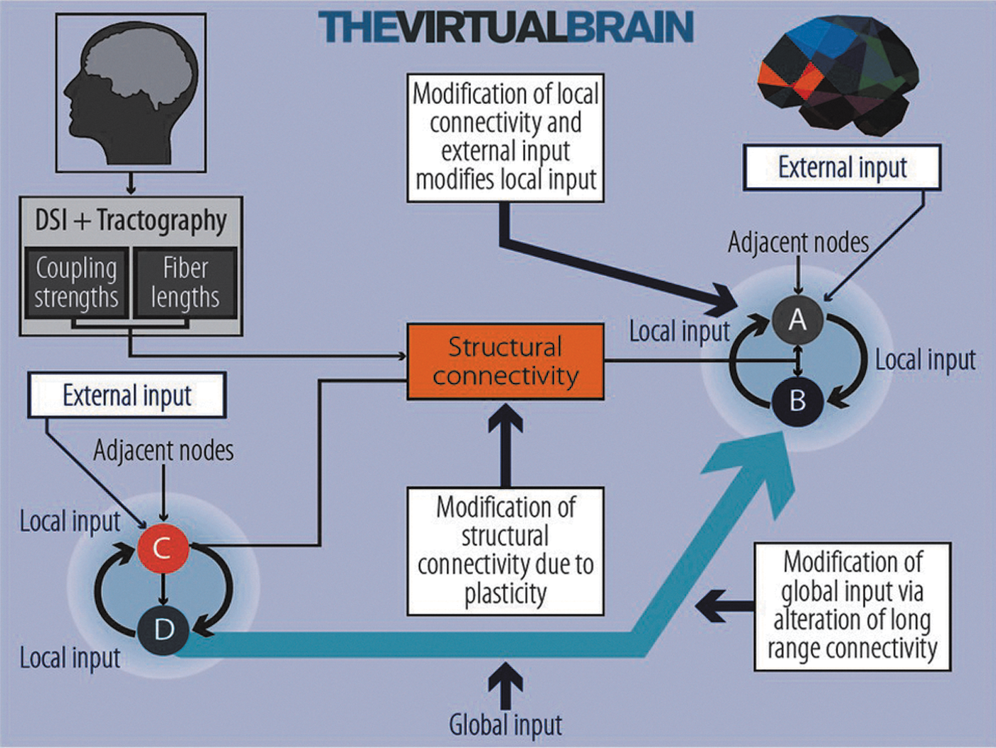
External input as well as local and global context shape ongoing brain dynamics. In the Virtual Brain (TVB) framework, we use informed structural connectivity (SC) (orange box) combined with local models described as nodes A, B, C, and D, respectively. TVB provides the choice of defining specific node dynamics using spiking attractor dynamics, firing rate dynamics, or oscillator models. The local models receive external time-varying input reflecting external stimuli, e.g. noisy input, external constant current input, local input from adjacent neural populations, and a global contextual input from distant populations. There are various ways to parametrically modulate the input received by an individual node; for example, by modifying SC, the local network connectivity (local scaling factor), long distance connectivity (global coupling scaling factor), and external input. Color images available online at www.liebertpub.com/brain

Table 1.

A Selection of Models Providing Important Insights into the Origin of Observed SpatioTemporal Pattern During Rest

RSN model	Node model	Network dynamics	Connectome data	Role of delays	Role of noise	BOLD correlations and EEG dynamics
Honey et al. (2007)	Conductance based model	Chaotic activity	Macaque single hemisphere	None	Yes	Multi-scale and dynamic
Ghosh et al. (2008a)	Fitzugh-Nagumo neurons	Asynchronous 10 Hz firing activity	Macaque n=38 regions	Yes	Yes	Slow oscillatory mode with high variability for sufficient coupling
Deco et al. (2009)	Wilson-Cowan model	Limit cycle with 40 Hz	Macaque n=38 regions	Yes	Yes	Cluster synchrony and slow fluctuation
Freyer et al. (2011)	Robinson neural field model	Subcrtical Hopf bifurcation	Cortex and thalamus; no spatial structure	None	Yes	Bistability of alpha rhythm and noise-driven critical dynamics
Deco and Jirsa et al. (2012) and Deco et al. (2013)	Spiking IF neurons, mean field reduced model, linear moment model	Asynchronus low stable firing pattern	Human n=66 brain areas	None	Yes	Ghost attractors and noisy explorations of multistable attractor landscape
Cabral et al. (2011)	Kuramoto oscillators	Slow fluctuation in the degree of synchrony	Human n=66 90 brain areas	Yes	None	Metastable dynamics and synchrony of modules
Ritter et al. (2013)	Stefenscu-Jirsa model	Noisy excursion, multi-stable dynamical landscape	Human n=96 brain areas	None	Yes	Metastable dynamics and noise-driven excursion of multistable attractor landscape

Models capturing underlying neurodynamic mechanisms and features of empirical observations in neuroimaging research using fMRI, magnetencephalography and EEG. In all models, structural information is extracted from databases compiling different types of tracing studies; for example, in the macaque cortex, this information is provided by the CoCoMac neuroinformatics platform (Kotter, 2004) or by tractography using DTI data (Nooner et al.) and DSI (Hagmann et al., 2008).

BOLD, blood oxygenation level dependent; DSI, diffusion spectrum imaging; DTI, diffusion tensor imaging; EEG, electroencephalography; fMRI, functional magnetic resonance imaging; IF, integrate-and-fire; RSN, resting state networks.

Single brain area spiking model

We introduce a network of integrate-and-fire (IF) spiking neurons with excitatory (α-amino-3-hydroxy-5-methyl-4-isoxazolepropionic acid [AMPA] receptors, N-methyl-D-aspartate [NMDA] receptors) and inhibitory populations with gamma-aminobutyric acid (GABA) receptor types. This spiking neuron model is similar to the one used in Brunel and Wang (2001) and Deco and Jirsa (2012). Each cortical region is modeled as a fully recurrently connected network comprising N_E excitatory neurons and N_I inhibitory neurons (Table 2). We describe the dynamical evolution of a single neuron's membrane potential V(t) that is driven by incoming total excitatory and inhibitory inputs of the same cortical area and the long-range excitatory input from directly connected brain areas. Hence, the time evolution of the membrane potential for an arbitrary neuron i obeys the following differential equation: \documentclass{aastex}\usepackage{amsbsy}\usepackage{amsfonts}\usepackage{amssymb}\usepackage{bm}\usepackage{mathrsfs}\usepackage{pifont}\usepackage{stmaryrd}\usepackage{textcomp}\usepackage{portland, xspace}\usepackage{amsmath, amsxtra}\pagestyle{empty}\DeclareMathSizes{10}{9}{7}{6}\begin{document} \begin{align*} C_m & \frac { dV_i ( t ) } { dt } = I_L - I^ { ext } _ { AMPA } - I_ { i , syn } \\ I_L & = - g_m ( V ( t ) - V_L) & ( 1 ) \end{align*} \end{document}

where g_m is the membrane leak conductance, C_m is the membrane capacitance, and V_L is the resting potential; membrane time constant is defined as \documentclass{aastex}\usepackage{amsbsy}\usepackage{amsfonts}\usepackage{amssymb}\usepackage{bm}\usepackage{mathrsfs}\usepackage{pifont}\usepackage{stmaryrd}\usepackage{textcomp}\usepackage{portland, xspace}\usepackage{amsmath, amsxtra}\pagestyle{empty}\DeclareMathSizes{10}{9}{7}{6}\begin{document}$$\tau_m = \frac { C_m } { g_m } $$ \end{document} .

Table 2.

Neurons, Connections, and Synaptic Parameters in Each Local Brain Area

Excitatory neurons		Inhibitory neurons		Synapses
N_E	400	N_I	100	V_E	0 mV
C_m	0.5 nF	C_m	0.2 nF	V_I	−70 mV
V_thershold	−50 mV	V_thershold	−50 mV	τ_AMPA,e.	5 msec
_Vreset	−55 mV	_Vreset	−55 mV	τ_AMPA,r.	5 msec
g_m	25 nS	g_m	20 nS	τ_NMDA,r	2 msec
V_L	−70 mV	V_L	−70 mV	τ_NMDA,g	100 msec
g_AMPA,ext	3.18 nS	g_AMPA,ext	2.08 nS	τ_GABA	10 msec
g_AMPA,rec	0.104 nS	g_AMPA,rec	0.081 nS	k	0.062
g_AMPA,rec	0.327 nS	g_AMPA,rec	0.307 nS	β	0.5 kHz
g_GABA	4.575 nS	g_GABA	3.514 nS	λ_NMDA	0.28
Plasticity parameters rhythmic input frequency
A₊	0.019	f=10 Hz
A₋	0.010
τ₊	20 msec
τ_-	20 msec

I_syn is the synaptic current and comprises AMPA currents, NMDA currents, and GABA-A currents as defined next. The spike is transmitted to other neurons, and the membrane potential is instantaneously reset to V_reset and further maintained there until a refractory period is reached τ_ref during which neurons are unable to produce further spikes.

Postsynaptic excitatory potentials are generated on the target neuron mediated via the conductance-based model specified by synaptic receptors, namely: glutamatergic AMPA external excitatory currents, AMPA, NMDA recurrent excitatory currents, and GABAergic recurrent inhibitory currents. The respective synaptic conduct g_AMPA,ext , g_AMPA,rec , g_NMDA,rec and g_GABA,rec , V_E , V₁ are excitatory and inhibitory reversal potentials, respectively. Each one of the current excitatory feed-forward input currents, recurrent excitatory as well as inhibitory synaptic currents are described next: \documentclass{aastex}\usepackage{amsbsy}\usepackage{amsfonts}\usepackage{amssymb}\usepackage{bm}\usepackage{mathrsfs}\usepackage{pifont}\usepackage{stmaryrd}\usepackage{textcomp}\usepackage{portland, xspace}\usepackage{amsmath, amsxtra}\pagestyle{empty}\DeclareMathSizes{10}{9}{7}{6}\begin{document} \begin{align*}& I_ { AMPA } ^ { ext } ( t ) = g_ { AMPA , ext } ( V_i ( t ) - V_E ) \mathop\sum_ { j = 1 } ^ { N_ { ext } } s_j^ { \,AMPA , ext } ( t ) \\ & I_ { syn } ^ { i } ( t ) = g_ { AMPA , rec } ( V_i ( t ) - V_E ) \mathop\sum_ { j = 1 } ^ { N_E } w_ { ij} s_j^ { \,AMPA , rec } ( t ) \\ &+ \frac { g_ { NMDA } ( V_i ( t) - V_E ) } { ( 1 + \lambda_ { NMDA } e^ { - kV_ { i } ( t ) } )} \mathop\sum_ { j = 1 } ^ { N_E } w_ { ij } s_j^ { \,NMDA , rec }( t ) \\& \quad+ g_ { GABA } ( V_i ( t ) - V_I ) \mathop\sum_ { j= 1 } ^ { N_I } w_ { ij } s_j^ { GABA , rec } ( t ) \tag { 2 } \end{align*} \end{document}

Dimensionless parameters w_ij are the synaptic weights of recurrent all-to-all connectivity between excitatory and inhibitory neurons in each local brain area. By modifying these weights, one can either up- or down regulate the four local connectivity strength parameters (w_EE , w_EI , w_IE , w_II ). Unless otherwise specified, synaptic weights of the local recurrent connectivity are held at fixed values throughout our simulation of models. The recurrent self-excitation w_EE =W ⁺=1.4 and the remaining three synaptic weights are w_EI =w_IE =w_II =1, respectively.

The fraction of open channels of neurons are given by the kinetics of the gating variables \documentclass{aastex}\usepackage{amsbsy}\usepackage{amsfonts}\usepackage{amssymb}\usepackage{bm}\usepackage{mathrsfs}\usepackage{pifont}\usepackage{stmaryrd}\usepackage{textcomp}\usepackage{portland, xspace}\usepackage{amsmath, amsxtra}\pagestyle{empty}\DeclareMathSizes{10}{9}{7}{6}\begin{document}$$s_j^I$$ \end{document} modeled as \documentclass{aastex}\usepackage{amsbsy}\usepackage{amsfonts}\usepackage{amssymb}\usepackage{bm}\usepackage{mathrsfs}\usepackage{pifont}\usepackage{stmaryrd}\usepackage{textcomp}\usepackage{portland, xspace}\usepackage{amsmath, amsxtra}\pagestyle{empty}\DeclareMathSizes{10}{9}{7}{6}\begin{document} \begin{align*} \frac { ds_j^I ( t ) } { dt } = - \frac { s_j^I }{ \tau_I } + \mathop\sum_p \delta ( t - t_j^ { \,p } ) , { \rm for} \ I = AMPA \ or \ GABA \tag { 3 } \end{align*} \end{document}

NMDA channels are represented by a separate decay and rise-time kinetics. The sums over index p represent all the spikes emitted by presynaptic neuron j at times \documentclass{aastex}\usepackage{amsbsy}\usepackage{amsfonts}\usepackage{amssymb}\usepackage{bm}\usepackage{mathrsfs}\usepackage{pifont}\usepackage{stmaryrd}\usepackage{textcomp}\usepackage{portland, xspace}\usepackage{amsmath, amsxtra}\pagestyle{empty}\DeclareMathSizes{10}{9}{7}{6}\begin{document}$$t_j^{\,p} \cdot \tau_{AMPA}$$ \end{document} and τ_GABA represent the decay times for AMPA and GABA synapses. τ_NMDA,rise and τ_NMDA,decay are the rise and decay time constants for the NMDA synapses in the model. The NMDA currents are voltage dependent, and they are modulated via intracellular magnesium concentrations that are defined as \documentclass{aastex}\usepackage{amsbsy}\usepackage{amsfonts}\usepackage{amssymb}\usepackage{bm}\usepackage{mathrsfs}\usepackage{pifont}\usepackage{stmaryrd}\usepackage{textcomp}\usepackage{portland, xspace}\usepackage{amsmath, amsxtra}\pagestyle{empty}\DeclareMathSizes{10}{9}{7}{6}\begin{document}$$x_j^{\,NMDA} ( t )$$ \end{document} \documentclass{aastex}\usepackage{amsbsy}\usepackage{amsfonts}\usepackage{amssymb}\usepackage{bm}\usepackage{mathrsfs}\usepackage{pifont}\usepackage{stmaryrd}\usepackage{textcomp}\usepackage{portland, xspace}\usepackage{amsmath, amsxtra}\pagestyle{empty}\DeclareMathSizes{10}{9}{7}{6}\begin{document} \begin{align*} & \frac { ds_j^ { \,NMDA } } { dt } = - \frac { s_j^ { \,NMDA } ( t ) } { \tau_ { NMDA , decay } } + \beta x_j^ { \,NMDA } ( t ) ( 1 - s_j^ { \,NMDA } ( t ) ) \\ & \frac { dx_j^ { \,NMDA } ( t ) } { dt } = - \frac { x_j^ { \,NMDA } ( t ) } { \tau_ { NMDA , rise } } + \mathop\sum_p \delta ( t - t_j^ { \,p }) . & ( 4 ) \end{align*} \end{document}

In addition, all neurons in the network receive an AMPA-mediated external background current derived from a Poisson process of uncorrelated spikes with time-varying firing rate \documentclass{aastex}\usepackage{amsbsy}\usepackage{amsfonts}\usepackage{amssymb}\usepackage{bm}\usepackage{mathrsfs}\usepackage{pifont}\usepackage{stmaryrd}\usepackage{textcomp}\usepackage{portland, xspace}\usepackage{amsmath, amsxtra}\pagestyle{empty}\DeclareMathSizes{10}{9}{7}{6}\begin{document}$$f_{ext}^ \lambda ( t )$$ \end{document} governed by a simple Brownian process given by \documentclass{aastex}\usepackage{amsbsy}\usepackage{amsfonts}\usepackage{amssymb}\usepackage{bm}\usepackage{mathrsfs}\usepackage{pifont}\usepackage{stmaryrd}\usepackage{textcomp}\usepackage{portland, xspace}\usepackage{amsmath, amsxtra}\pagestyle{empty}\DeclareMathSizes{10}{9}{7}{6}\begin{document} \begin{align*} \frac { df_ { ext } ^ \lambda } { dt } = \frac {(\, f_ { ext } ^ \lambda ( t ) - f_0 ) } { \tau_n } + \sigma_f \sqrt \frac { 2 } { \tau_n } dW ( t ) \tag { 5 } \end{align*} \end{document}

where τ_n =30 msec, baseline firing rate=2.18 kHz (background). Local and global connectivity parameters are given in Table 2. Parameter values in Table 2 are modified from Brunel and Wang (2001)—where the network balance is shifted more toward an inhibitory regime—to incorporate local balance of excitatory and inhibitory synaptic currents as shown in Deco and Jirsa (2012), Albantakis and Deco (2011), and Deco and coworkers (2013c, 2014). Parameters for the single cortical area neuronal synapse model are summarized in Table 2. One of the key motivations for the choice of single area parameters as shown in Table 2 was to keep the uncoupled local area network to fire asynchronously at around 3–4 Hz, which closely resembles the biological range of spontaneous firing activity given in any isolated cortical region (Haider et al., 2006). Hence, this asynchronous spontaneous firing rate is maintained at about 3–4 Hz when isolated from the global network and in the absence of plasticity and brain state-dependent feed-forward drive. This type of local balance of excitation and inhibition in local cortical networks is sufficient to achieve oscillations in the desired frequency range, maximal synchrony and criticality in the resting-state dynamics (Poil et al., 2012). The balance (local excitation-inhibition ratio) impacts the spontaneous and evoked large-scale brain dynamics (Deco et al., 2014).

Single brain area represented by a DMF model

To model the RSN dynamics and prediction of empirical functional connectivity at the macroscopic level, Deco and coworkers (2013b, 2014) proposed a large-scale DMF model derived from the spiking model described earlier. As shown in Deco and associates (2014), the reduced DMF model consistently expresses the time evolution of the ensemble activity of the different excitatory and inhibitory neural populations building up the spiking network. In the DMF approach, each population's firing rate depends on the input currents into that population. The input currents, in turn, depend on the cortical pool population firing rates. The populations firing rate can be determined by a reduced system of coupled nonlinear differential equations that are driven by the respective input currents. The large-scale model connects these local sub-networks according to the SC matrix defined by the anatomical connections between those brain areas in the human, as obtained by diffusion spectrum imaging (DSI) and described earlier. The inter-area connections are established as long-range excitatory synaptic connections either exclusively between excitatory pools of different areas or both between excitatory pools as well as excitatory pools and inhibitory pools of different areas. Inter-areal connections are weighted by the strength specified in the SC matrix, denoting the density of fibers between those regions and by the state parameter global coupling strength G. When each cortical area is embedded in a large-scale network, their global brain dynamics are governed by the following sets of coupled stochastic nonlinear differential equations for the excitatory pool and the inhibitory pool, respectively: \documentclass{aastex}\usepackage{amsbsy}\usepackage{amsfonts}\usepackage{amssymb}\usepackage{bm}\usepackage{mathrsfs}\usepackage{pifont}\usepackage{stmaryrd}\usepackage{textcomp}\usepackage{portland, xspace}\usepackage{amsmath, amsxtra}\pagestyle{empty}\DeclareMathSizes{10}{9}{7}{6}\begin{document} \begin{align*} \frac { dE_n^ { exc } } { dt } &= - \frac { E_n^{ exc } } { \tau_ { exc } } + ( 1 - E_n^ { exc } ) \gamma r_n^ { exc } + \sigma v_n ( t ) , \\ \frac { dE_n^ { inh } } { dt } &= - \frac { E_n^ { inh } } { \tau_ { inh } } + r_n^ { inh } + \sigma v_n ( t ) , \\ r_n^T &= H^T ( I_n^T ) = \frac { a_T ( I_n^T ) - b_T } { 1 - \exp ( - d_T ( a_TI_n^T - b_T ) ) } \\ T &= exc , inh \\ I_n^ { exc } &= I_ { ext } + W^ { + } J_ { NMDA } E_n^ { exc }+ GJ_ { NMDA } \mathop\sum_j C_ { nj } E_j^ { exc } - J_n E_n^ { inh } \\ I_n^ { inh } &= J_ { NMDA } E_n^ { exc } - E_n^ { inh } &( 6 ) \end{align*} \end{document}

In Eq. (6), \documentclass{aastex}\usepackage{amsbsy}\usepackage{amsfonts}\usepackage{amssymb}\usepackage{bm}\usepackage{mathrsfs}\usepackage{pifont}\usepackage{stmaryrd}\usepackage{textcomp}\usepackage{portland, xspace}\usepackage{amsmath, amsxtra}\pagestyle{empty}\DeclareMathSizes{10}{9}{7}{6}\begin{document}$$r_n^T$$ \end{document} describes the excitatory and inhibitory population firing rate in each cortical region. \documentclass{aastex}\usepackage{amsbsy}\usepackage{amsfonts}\usepackage{amssymb}\usepackage{bm}\usepackage{mathrsfs}\usepackage{pifont}\usepackage{stmaryrd}\usepackage{textcomp}\usepackage{portland, xspace}\usepackage{amsmath, amsxtra}\pagestyle{empty}\DeclareMathSizes{10}{9}{7}{6}\begin{document}$$E_n^{exc}$$ \end{document} , \documentclass{aastex}\usepackage{amsbsy}\usepackage{amsfonts}\usepackage{amssymb}\usepackage{bm}\usepackage{mathrsfs}\usepackage{pifont}\usepackage{stmaryrd}\usepackage{textcomp}\usepackage{portland, xspace}\usepackage{amsmath, amsxtra}\pagestyle{empty}\DeclareMathSizes{10}{9}{7}{6}\begin{document}$$E_n^{inh}$$ \end{document} describe the average excitatory and inhibitory synaptic strength in each local area n. \documentclass{aastex}\usepackage{amsbsy}\usepackage{amsfonts}\usepackage{amssymb}\usepackage{bm}\usepackage{mathrsfs}\usepackage{pifont}\usepackage{stmaryrd}\usepackage{textcomp}\usepackage{portland, xspace}\usepackage{amsmath, amsxtra}\pagestyle{empty}\DeclareMathSizes{10}{9}{7}{6}\begin{document}$$I_n^{exc}$$ \end{document} , \documentclass{aastex}\usepackage{amsbsy}\usepackage{amsfonts}\usepackage{amssymb}\usepackage{bm}\usepackage{mathrsfs}\usepackage{pifont}\usepackage{stmaryrd}\usepackage{textcomp}\usepackage{portland, xspace}\usepackage{amsmath, amsxtra}\pagestyle{empty}\DeclareMathSizes{10}{9}{7}{6}\begin{document}$$I_n^{inh}$$ \end{document} represent the input currents to the excitatory and inhibitory population, respectively. \documentclass{aastex}\usepackage{amsbsy}\usepackage{amsfonts}\usepackage{amssymb}\usepackage{bm}\usepackage{mathrsfs}\usepackage{pifont}\usepackage{stmaryrd}\usepackage{textcomp}\usepackage{portland, xspace}\usepackage{amsmath, amsxtra}\pagestyle{empty}\DeclareMathSizes{10}{9}{7}{6}\begin{document}$$I_{ext}$$ \end{document} is the external drive to the cortical neurons. W⁺ =1.4 represents the self-excitatory recurrent synaptic strength as in the spiking model. C_nj is the SC matrix that connects individual brain areas, where n and j are two arbitrary brain areas. In this model, only excitatory-excitatory long-range connections are taken into account; hence, global coupling strength appears only in the first equation of (7) for the description of the excitatory population firing rates. Neuronal input-output relationship is expressed as sigmoidal and denoted as \documentclass{aastex}\usepackage{amsbsy}\usepackage{amsfonts}\usepackage{amssymb}\usepackage{bm}\usepackage{mathrsfs}\usepackage{pifont}\usepackage{stmaryrd}\usepackage{textcomp}\usepackage{portland, xspace}\usepackage{amsmath, amsxtra}\pagestyle{empty}\DeclareMathSizes{10}{9}{7}{6}\begin{document}$$H_n ^{( T )}$$ \end{document} _, where T=exc,inh pools, respectively, in each cortical region n. This function converts incoming inputs to firing rates. Additional paramters are the excitatory recurrent coupling strength J_NMDA =0.15(nA), the kinetic parameters γ=0.0641/1000, τ_exc =100ms, τ_inh =10ms, and the local feedback inhibitory coupling J_n =1. Other parameters that are specific to calculation of input currents are as follows: \documentclass{aastex}\usepackage{amsbsy}\usepackage{amsfonts}\usepackage{amssymb}\usepackage{bm}\usepackage{mathrsfs}\usepackage{pifont}\usepackage{stmaryrd}\usepackage{textcomp}\usepackage{portland, xspace}\usepackage{amsmath, amsxtra}\pagestyle{empty}\DeclareMathSizes{10}{9}{7}{6}\begin{document} \begin{align*}a_{exc} & = 310 ( nC^{ - 1} ) , b_{exc} = 125 ( Hz) , d_{exc} = 0.16 ( s ) \\ a_{inh} & = 615 ( nC^{ - 1} ) , b_{inh} = 177 ( Hz ) , d_{inh} = 0.087 ( s ) \end{align*} \end{document}

In order to obtain maximum excitatory firing rate, the global coupling strength is varied as a free parameter. The result is displayed in Figure 2D. Simulation of the global model with a range of low global coupling strength G=[0.0 – 0.5] shows spontaneous population activity with an excitatory mean firing rate of 3–4 Hz, which is what we have obtained for the global spiking model by varying the global coupling strength parameter. At even higher values of G=[1.5 – 4.0] both low and high population firing rates co-exist as steady-state solutions. For coupling above G>4.0, fixed point attractors destabilize and the system enters into a regime coinciding with a high mean excitatory population firing rate. This is shown for both the spiking model and the DMF model separately to visualize their dynamical transition properties with a range of control parameters. The critical values for phase transition are shown in Figure 2C and D as well as in Figure 8.

FIG. 2.

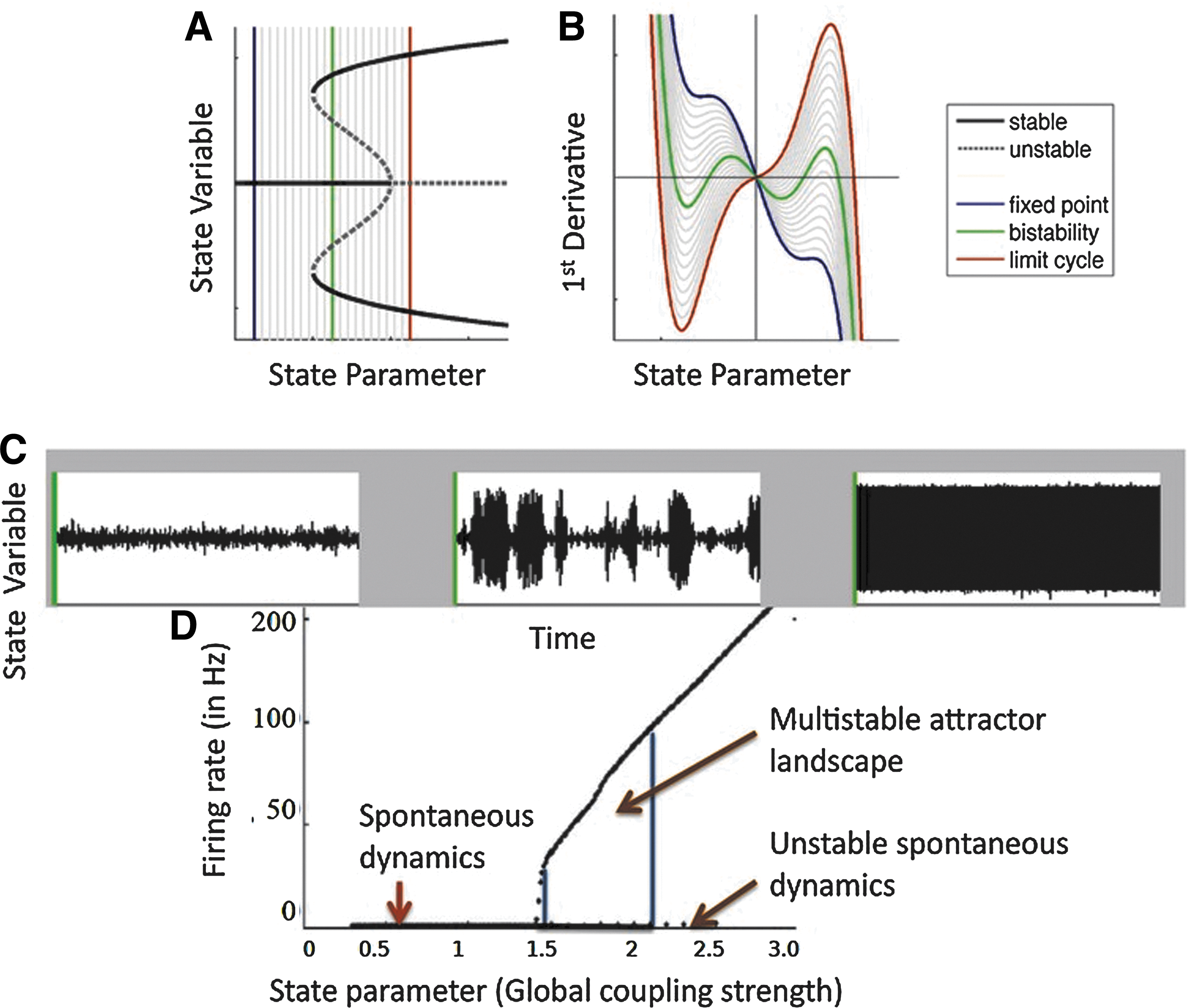
Resting-state dynamical landscape. Figure adapted and modified from Freyer and coworkers (2012b). (A) Dynamical instability in the form of a subcritical Hopf bifurcation and the emergence of steady states. The system exhibits bistability as a function of the control parameter driven by nonlinearities present in the state variables. (B) First derivatives or slopes of the state variables showing the corresponding inflection points on the displayed curve, that is, maxima and minima of steady state solutions. In the bistable scenario depicted with a green solid line, the system exhibits double well potential form with two prominent bumps. (C) Noise-driven exploration of possible solutions. Three different ongoing dynamics are observed: subthreshold fluctuations around low firing steady state followed by a multistable attractor landscape (coexistence of low and high firing rate fluctuations) and subsequently transitions to high amplitude firing rate dynamics via change of the state parameter “global coupling strength.” (D) The state variable “population-firing rate” is a function of the state parameter “global coupling strength.” Two stable solutions on either side of the bifurcation points are visible. One is the low amplitude asynchronous stable spontaneous solution, and the other is the high amplitude unstable spontaneous dynamics. In between, the resting-state spontaneous activity reflects a multi-stable attractor landscape and exhibits structure fluctuations as shown (C, middle). Color images available online at www.liebertpub.com/brain

Numerical procedure

The local pool represented by a cortical spiking IF model when uncoupled from the global network is simulated using Python 2.7, scipy, and numpy. Resting-state spontaneous activity and the mean firing rate of each cortical module are obtained using a numerical integration procedure in the C code environment. STDP in local cortical areas is implemented using an exponential STDP class as implemented in Brian, a spiking network simulator, version 1.4. Time-frequency domain analysis is carried out on the LFP-like activity from cortical pools using the custom-made MATLAB code. BOLD signals are simulated using hemodynamic response function, and covariance between relevant brain areas is estimated using custom-made MATLAB scripts. DMF model with fully connected brain areas is simulated using custom-made MATLAB scripts that are available from the open source computational models database http://senselab.med.yale.edu/ModelDB. In the near future, we will incorporate relevant parts of our script in TVB as well.

Alteration of Dynamic Landscape Due to Locally Restricted Plasticity

In principle, it is possible to implement plasticity in both spiking and DMF models while taking advantage of a mechanism such as the balance of excitatory and inhibitory currents as recently proposed by Deco and coworkers (2014). This mechanism can be introduced in the DMF to clip the local area asynchronous firing rate to 3–4 Hz. Plasticity crucially depends on neurons with a similarly timed activity. Hence, in this study, we are more focused on the presynaptic-postsynaptic spike timing difference and the role of feed-forward input oscillations for the spiking of the output neurons at the precise phases of the input oscillations. Hence, amplification of network firing rates can be realized via appropriate modifications of spike timing in a mean field rate model setting. For the investigation of various effects of plasticity, we chose a spiking neuron model with a biophysically realistic attractor network. This attractor network as shown in Eqs. (1 –5) is a dynamical system with an intrinsic tendency to settle in stationary states—also called “attractors.” Attractors are typically characterized by stable patterns of firing (Fig. 2). Individual neurons are modeled as IF spiking neurons with biologically realistic excitatory (AMPA and NMDA) and inhibitory (GABA-A) synaptic receptor types. Realistic description of the synapses and nonlinear dependency of the synaptic current on the excitatory currents received from other neurons allow for including STDP. However, integrating the full spiking model is computationally expensive. This makes the exploration of the parameter space to find the parametric conditions matching the experimental findings a challenge. We know from empirical data that learning alters the rs-FC by restructuring connections employing Hebbian-like rules (Freyer et al., 2012a; Harmelech et al., 2013). We aim here to reproduce similar effects with a large-scale model implementing local STDP. The implementation of local plasticity at the node level is motivated from several relevant studies of microcircuit modeling (Morrison et al., 2007; Vogels et al., 2011). The implication for decoding of afferents in readout neuronal assemblies has been recently demonstrated, in studies that combine the PoFC and STDP mechanisms (Deco et al., 2011; Masquelier et al., 2009). It still remains an open question how these mechanisms may influence learning-related changes in distant brain areas. Recently, STDP was introduced in hierarchically modular realistic brain networks comprising leaky IF neurons (Rubinov et al., 2011) to investigate emergent criticality in spontaneous network dynamics. In this study, authors have found that STDP enabled a phase transition from random subcritical dynamics to ordered supercritical dynamics, hence broadening the parameter regime in which balanced criticality reigns. We here go beyond this work by (1) exploring the role of ongoing states for STDP-related local reorganization and (2) illuminating the spatial (global) effects that evolve from local plastic changes and resulting altered dynamic repertoire at the node level.

Implementing STDP and PoFC in a spike model

In this section, we test the hypothesis that background oscillations alter capability for plasticity in a connected network of cortical neurons. We build a spike model with STDP, where the cortical layer receives about 1000 thalamic afferent external inputs mediated via conductance-based excitatory AMPA synapses (Fig. 3). In the present spike model, node level dynamics is asynchronous with a firing rate of 3–4 Hz in the absence of an oscillatory input—as shown in Figure 4. In addition, cortical populations receive a periodic modulation of feed-forward thalamic input spikes generated at a rate of the alpha frequency (8–12 Hz). Put differently, afferent spike output from thalamus to cortex is modulated via a sinusoid as shown in Figure 3D. As a consequence, firing rates of the inputs change on a timescale highly relevant to STDP. Thalamic input spike trains are approximated as a continuous sinusoid. Randomness in the thalamic spike phases is introduced via a Poisson process. About 1000 thalamic spike trains drive a cortical node represented by IF neurons. Plasticity introduced between thalamic input layer and cortex induces a systematic change in the local microcircuit on a short time scale of milliseconds. This is carried out by systematic potentiation and depression of local cortico-thalamic excitatory synaptic weights w_tc and altering recurrent connectivity between excitatory neurons (Figs. 4 and 5). In the spiking model, the recurrent self-excitation within each excitatory population is given by the weight w_EE =W ⁺ and recurrent all-to-all connectivity between excitatory-inhibitory population is given by the weights w_EI =w_IE =w_II =1 and further described in detail in the spiking model section. We include plasticity in the local AMPA receptor-mediated excitatory-excitatory synapses between thalamus and cortical area S1 neurons with synaptic weight w_tc between thalamus and cortex. Recurrent self-excitation is used as a fixed parameter in the node model with and without plasticity (Deco and Jirsa, 2012). In this model, thalamocortical feed-forward synaptic weight changes in the excitatory synapses due to plasticity serve as a critical control parameter. We assume that local excitatory synapses between pyramidal cells have at least two distinct conductance states due to plasticity: a high conductance state resulting from long term potentiation (LTP) of AMPA receptors at the postsynaptic site as described by Eq. (4), and conversely a low conductance state due to long term depression (LTD) of AMPA receptors (Brunel, 2003). Transitions from a low conductance to a high conductance state can be mediated by Hebbian plasticity, that is, selective potentiation and depression of synapses (Brunel, 2003; Mikkelsen et al., 2013). In our work, LTP/LTD windowing functions are based on those proposed by Song et al. (2000). LTP/LTD can be elicited by activating NMDA-type glutamate receptors, typically by the coincident activity of pre- and postsynaptic neurons. The windowing functions describe the time window when consequences of the near-coincidence of pre- and postsynaptic neuronal activity take place. Figure 3 illustrates a model combining oscillatory input patterns with cortical spiking IF neurons equipped with local STDP. The local neural population comprising excitatory and inhibitory spiking neuron populations receives rhythmic spike inputs from multiple neurons—1000 input neurons are shown in Figure 3A. Figure 3C illustrates how Hebbian plasticity is realized through STDP and depends on the relative timing of pre-and postsynaptic spikes. In addition, here we employ a precise relationship between phase of the background oscillations and the spike phase of output neurons. This is schematically illustrated in Figure 3D. If the phase of the background oscillations, that is, phase of oscillatory LFP activity, and the spike phase, that is, phase of oscillatory postsynaptic spikes (phase delay A₋ or advance A ₊) matches, then the synaptic recurrent excitatory weights are updated via a linear additive rule as proposed by Song et al. (2000) shown in Figure 3D. STDP exploits this precise relationship between LFP to spike phase and has previously been successfully employed as a parsimonious learning mechanism to demonstrate stable phase locking in a feed-forward network model (Muller et al., 2011). 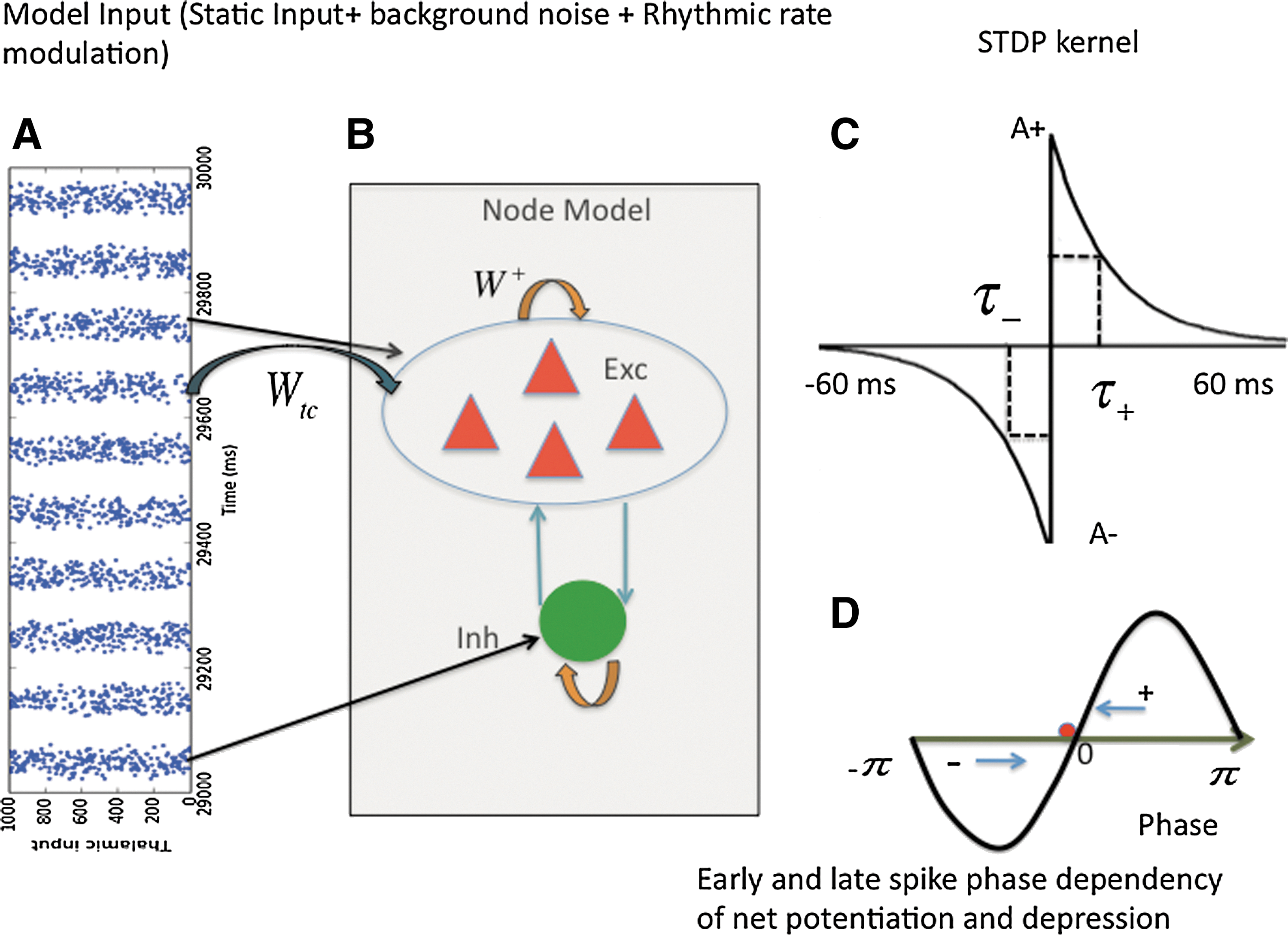The synaptic AMPA kinetics is governed by the following equations: \documentclass{aastex}\usepackage{amsbsy}\usepackage{amsfonts}\usepackage{amssymb}\usepackage{bm}\usepackage{mathrsfs}\usepackage{pifont}\usepackage{stmaryrd}\usepackage{textcomp}\usepackage{portland, xspace}\usepackage{amsmath, amsxtra}\pagestyle{empty}\DeclareMathSizes{10}{9}{7}{6}\begin{document} \begin{align*} \frac { ds_j^ { \,AMPA , ext } } { dt } & = - \frac { s_j^ { \,AMPA , ext } } { \tau_ { exc } } + \mathop\sum_p \delta ( t - t_j^ { \,p } ) \\ I^ { ext } { _ { AMPA } ( t ) } & = g_ { AMPA , ext } ( V_i ( t ) - V_E ) \mathop\sum_ { j = 1 } ^ { N_ { ext } } w_ { tc , ij } s_j^ { \,AMPA , ext } ( t ) & ( 7 ) \end{align*} \end{document}

FIG. 3.

Interplay between rhythmic input and spike-timing dependent plasticity (STDP) modulates learning at the node level. (A) One thousand periodically modulated Poisson-process spike inputs to a neural population model. (B) Population model comprising excitatory neurons (red) and inhibitory neurons (green). For simplicity, a few neurons are shown. Recurrent weights are indicated by blue arrows, and self-connections are indicated by yellow arrows. (C) The STDP kernel proposed for our work is a piecewise exponential function of pre- and postsynaptic spike times (t_post − t_pre ) based on (Song et al., 2000); τ₊ and τ₋ are the STDP time constants for long term potentiation (LTP) and long term depression (LTD) (LTP/LTD). A ₊ and A ₋ are the maximal changes for synaptic weights as a function of maximum weight updates denoted as w_max. (D) Weight change as a function of output spike phase. A late phase spike receives a net potentiation, and conversely an early phase spike receives net depression. The fixed point of this system is shown with a red dot. If the spike phase is at the fixed point of this system, no net update in weights occurs. Color images available online at www.liebertpub.com/brain

FIG. 4.

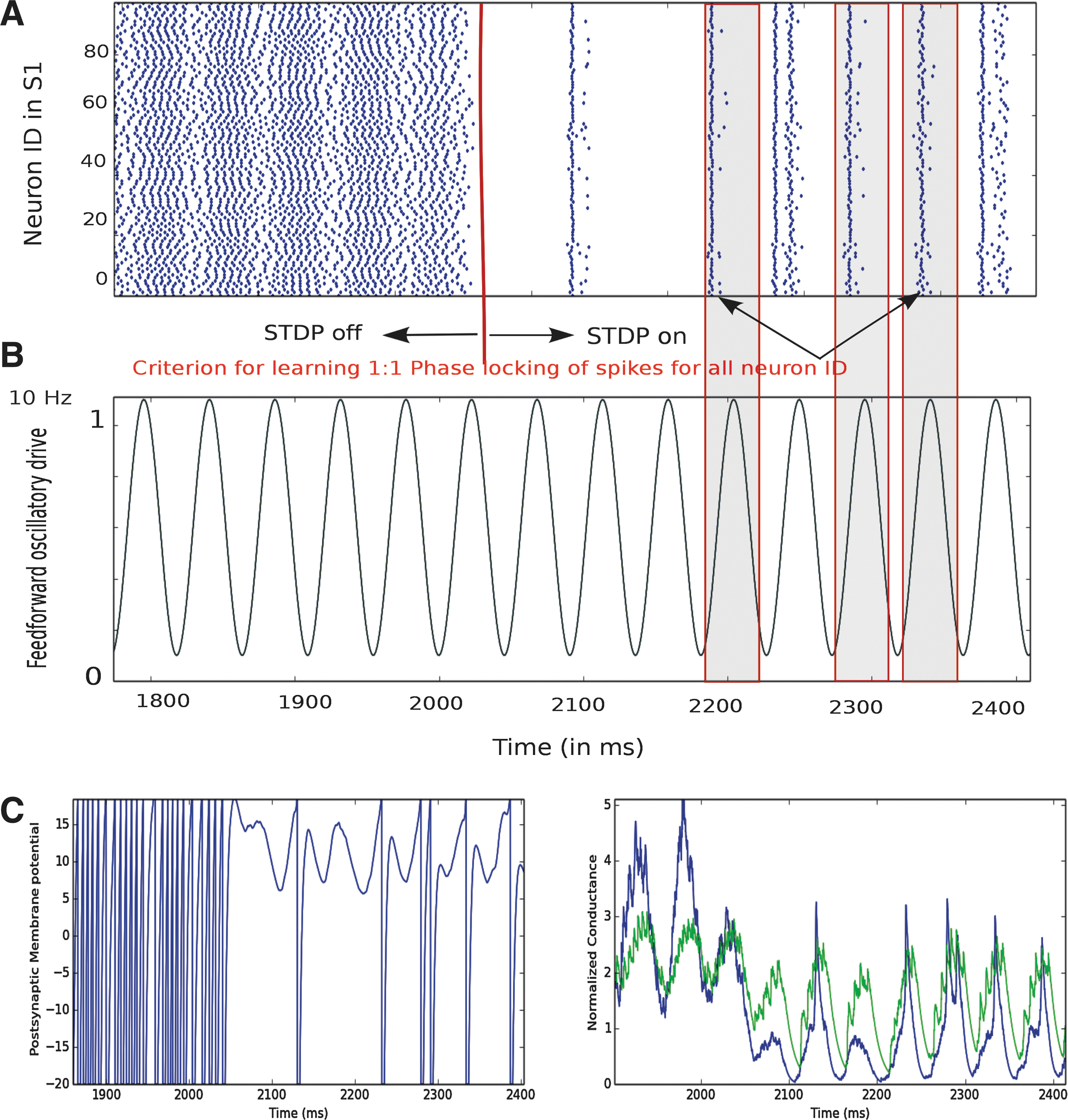
Learning with STDP in a local population S1 cortical integrate-and-fire (IF) neuron model with feed-forward oscillatory thalamic drive at alpha frequency around 10 Hz. A primary somatosensory cortical network neuron group is simulated for a total duration of 12 sec. STDP is turned on after about 2000 msec of simulation time (shown with a red marker). For clarity, 1800–2400 msec of cortical output activity are shown. Intrinsic network parameters are the same as shown in Table 2. (A) Raster plot of population spikes from 100 cortical neurons. Before 2000 msec, when STDP is off, cortical output exhibits asynchronous spiking activity independent of the phase of oscillations of thalamic input drive. When STDP is turned on after 2000 msec, cortical neurons start exhibiting a precise phase of firing (1:1 phase locking—a criterion that is used in this study for learning in local population spikes) with silence corresponding to phasic inhibition. (B) Simulated thalamic oscillatory drive (green) approximated as a sinusoid is plotted for the entire duration. Here, those spike times are shaded with a gray box, where 1:1 phase locking (learning in output populations) for all neuron IDs in S1 population is observed. (C) Simulated postsynaptic membrane potential is shown before and after STDP (18–2400 msec), which is in concordance with the population response, that is, before STDP membrane potential oscillates due to oscillatory feed-forward thalamic input; however, membrane potential reaches a threshold of −20 mV once in every cycle (no phase preference at all). After STDP (after 2000 msec), postsynaptic membrane response is strongly modulated via the input phase. Membrane potential reaches a threshold only when there is potentiation due to phase matching of spikes at the peak of the input oscillation cycle. (C) Excitatory synaptic conductance (in blue), inhibitory synaptic conductance (green) are shown. Effect of phasic inhibition is strongly present in the temporal response of conductance. Before STDP, excitatory conductance is typically higher than the inhibitory conductance due to the feed-forward excitatory drive, resulting in a number of spikes at arbitrary spike times as displayed in the spike raster plot (A). After STDP, excitatory and inhibitory conductance shows strong phase modulation. Potentiation leads to a homeostatic balance between excitatory-inhibitory conductance, leading to phase locking of spikes as shown in the raster plot. However, depotentiation of thalamocortical weight leads to lowering of the excitatory drive received by the cortical neurons and resulting in strong lateral inhibition as shown in green (between 2000–2400 msec) and silencing of cortical output as shown in the raster plot (A). Color images available online at www.liebertpub.com/brain

FIG. 5.

Alteration of thalamus-S1 synaptic weights (coupling strength) due to STDP, with and without brain state dependent input. Here, for clarity, only 100 excitatory presynaptic thalamic inputs are shown. (A) Connectivity changes between excitatory pre- and postsynaptic neuron pairs for the case of STDP applied for 10 seconds in the absence of rhythmic input. Synaptic weights are normalized between 0 and 1. Depressed synapses are color coded in blue (weight=0) and conversely potentiated synapses are color-coded in red (weight=1). (B) Connectivity changes between neuron pairs are shown for the combination of rhythmic input and STDP. Without rhythmic input, effectively, there are no input patterns to learn, hence, almost all excitatory synaptic weights are close to 1. With rhythmic modulation of the rate of thalamic presynaptic input afferent spikes, structural connectivity gets modified between thalamus and primary somatosensory cortex S1 as displayed in the layout of connectivity between pre- and postsynaptic neurons. Local clustering shapes the output dynamics of the postsynaptic population, i.e. here of S1. Color images available online at www.liebertpub.com/brain

Input connections to the IF neuron are mediated by exponential synapses with excitatory-excitatory corticothalamic synaptic weights w_tc without delays. When a presynaptic spike occurs, the excitatory synaptic weight is incremented by an amount w. The STDP rule is implemented with all-to-all spike pairings (Song et al., 2000). The synaptic weights are restricted to a range between 0 and w_max . For a given spike pairing with temporal difference x (spike time window), the synapse between the pre- and postsynaptic neurons is modified according to w_tc =w+f(x)w _max. Thus, the value of the STDP window is given by a piecewise exponential function f(x) for a given temporal difference x between pre- and postsynaptic spike times. Further, relative spike times determine the percentage of w_max added to the feed-forward corticothalamic synaptic weights w_tc . In our simulation, when a presynaptic spike occurs in the input, the fraction of open AMPA receptor channels is updated as \documentclass{aastex}\usepackage{amsbsy}\usepackage{amsfonts}\usepackage{amssymb}\usepackage{bm}\usepackage{mathrsfs}\usepackage{pifont}\usepackage{stmaryrd}\usepackage{textcomp}\usepackage{portland, xspace}\usepackage{amsmath, amsxtra}\pagestyle{empty}\DeclareMathSizes{10}{9}{7}{6}\begin{document}$$s_j^{\,AMPA , ext} \rightarrow s_j^{\,AMPA , ext} + w_{tc}$$ \end{document} . Since we study a plastic system with intrinsic stability in the coupling between STDP and oscillations, it is not necessary to include a stabilizing mechanism in the STDP rule, provided that the learning rate A ₊ is a reasonable value. We first assume an STDP rule with linear, all-to-all spike pairings. After previous theoretical work on STDP (Carroll et al., 2014; Kilpatrick and Bressloff, 2010; Song et al., 2000), we formulate the STDP rule as a piecewise exponential function: \documentclass{aastex}\usepackage{amsbsy}\usepackage{amsfonts}\usepackage{amssymb}\usepackage{bm}\usepackage{mathrsfs}\usepackage{pifont}\usepackage{stmaryrd}\usepackage{textcomp}\usepackage{portland, xspace}\usepackage{amsmath, amsxtra}\pagestyle{empty}\DeclareMathSizes{10}{9}{7}{6}\begin{document} \begin{align*}f ( x ) = \begin{cases} A_ { + } e^ { - \frac { x }{ \tau_ + } } , x > 0 \\ A_ { - } e^ { - \frac { x } { \tau_ { -} } } , x < 0 \end{cases} \tag { 8 } \end{align*} \end{document}

where x is defined as the difference in pre- and postsynaptic spike times (t_post − t_pre ), τ₊ and τ₋ are the STDP time constants for potentiation and de-potentiation, A ₊ is the amount of potentiation for an optimally potentiating pre-post pairing, and A ₋ is the same for a de-potentiating post-pre pairing. The ratio of de-potentiation to potentiation (A ₋τ₋/A ₊τ₊) will be termed the STDP ratio. For the case of identical time constants considered here, we write (A ₋/A ₊). The value of the function f(x) determines the percent change for a synaptic weight on a given pairing, relative to w_max . Each of the input neurons in Figure 3 is modeled as an oscillating inhomogeneous Poisson process. In Figure 3A, we show 1000 periodically modulated Poisson process spike inputs. The number of inputs is chosen as a compromise between biological realism and computational feasibility. Inputs are fed to the IF neuron by exponential, current-based synapses with a 5-ms decay time constant. As shown in the scheme in Figure 3D, recurrent weights are potentiated and depressed depending on the phase of the background oscillation. By default, the local node model is in a balanced Ex/Inh regime for intrinsic network parameter combinations characterized by low-amplitude asynchronous firing activity. When input oscillations are in the alpha frequency range yielding the most prominent spontaneous oscillations of the human brain, the presynaptic firing rate changes on a time scale relevant for the STDP time window Δt=0 to 5 msec (Babadi and Abbott, 2013; Caporale and Dan, 2008). A defining feature of STDP is very high temporal asymmetry (Guetig et al., 2003). When a presynaptic spike precedes the postsynaptic spike in time, then the synapse between the two is potentiated (pre-post pairing); while in the converse scenario, the synapse between the two is depressed (post-pre pairing). The interplay between thalamic input in the presence of oscillations and STDP is illustrated with a simulation of a node model representing primary somatosensory cortical area S1 composed of 100 excitatory neurons and 25 inhibitory IF spiking neurons. The node model is simulated for a total duration of 12 sec. STDP is turned on after 2000 msec of simulation time. The network runs for another 10 sec. In Figure 4, for clarity, the simulation results for cortical output neurons are shown for the time period 1800 to 2400 msec. Intrinsic network parameters are the same as displayed in Table 2. In Figure 4A, a raster plot of population spikes from 100 cortical excitatory neurons is shown. Before 2000 msec, cortical output exhibits asynchronous spiking activity even in the presence of oscillations in the thalamic input. When STDP is turned on after 2000 msec, cortical neurons start exhibiting a precise phase of firing, that is, phase locking, followed by transient events of silence that corresponds to phasic inhibition. If the output spike occurs at the trough of the input oscillation cycle, that is, “early,” it leads to de-potentiation in the cortico-thalamic synaptic weights w_tc in accordance with phase-dependent STDP. In contrast, when the spike occurs at the peak of input oscillation cycle, that is, “late,” this leads to net potentiation in the cortico-thalamic synaptic weights (Fig. 3). In Figure 4B, the simulated postsynaptic membrane potential is shown both before and after STDP. Before STDP, the membrane potential oscillates due to oscillatory feed-forward thalamic input. The membrane potential reaches the threshold of −20 mV once in every cycle. There is no phase preference. After STDP, that is, after 2000 msec, the postsynaptic membrane potential is modulated by the input phase. The membrane potential reaches the threshold only when there is potentiation due to phase matching of spikes at the peak of the input oscillation cycle. In Figure 4C, excitatory synaptic conductance (blue) and inhibitory synaptic conductance (green) are shown. The effect of phasic inhibition is strongly present in the temporal dynamics of both conductance types. Before STDP, excitatory conductance is typically higher than the inhibitory conductance due to the feed-forward excitatory drive, resulting in a number of spikes at arbitrary times as shown in the population raster plot between 1800 and 2000 msec. After STDP, excitatory conductance as well as inhibitory conductance exhibits strong phase modulation. Potentiation in this scenario leads to a homeostatic balance between excitatory-inhibitory conductance, leading to phase locking of spikes as shown in the raster plot. However, depression in corticothalamic synaptic weights leads to lowering of the excitatory drive received by the cortical neurons and thus resulting in a strong cortical, that is, recurrent or lateral inhibition dominating the excitatory conductance as shown in green (between 2000 and 2400 msec). As a consequence, silencing takes place in cortical output neurons at those time points as shown in the raster plot in Figure 4A. An increase in phase locking of spikes to the background input oscillatory phase (LFP-spike precise phase coupling) after STDP paves way for learning in the local node model that, in turn, plays a crucial role in influencing network dynamics in the globally connected nodes.

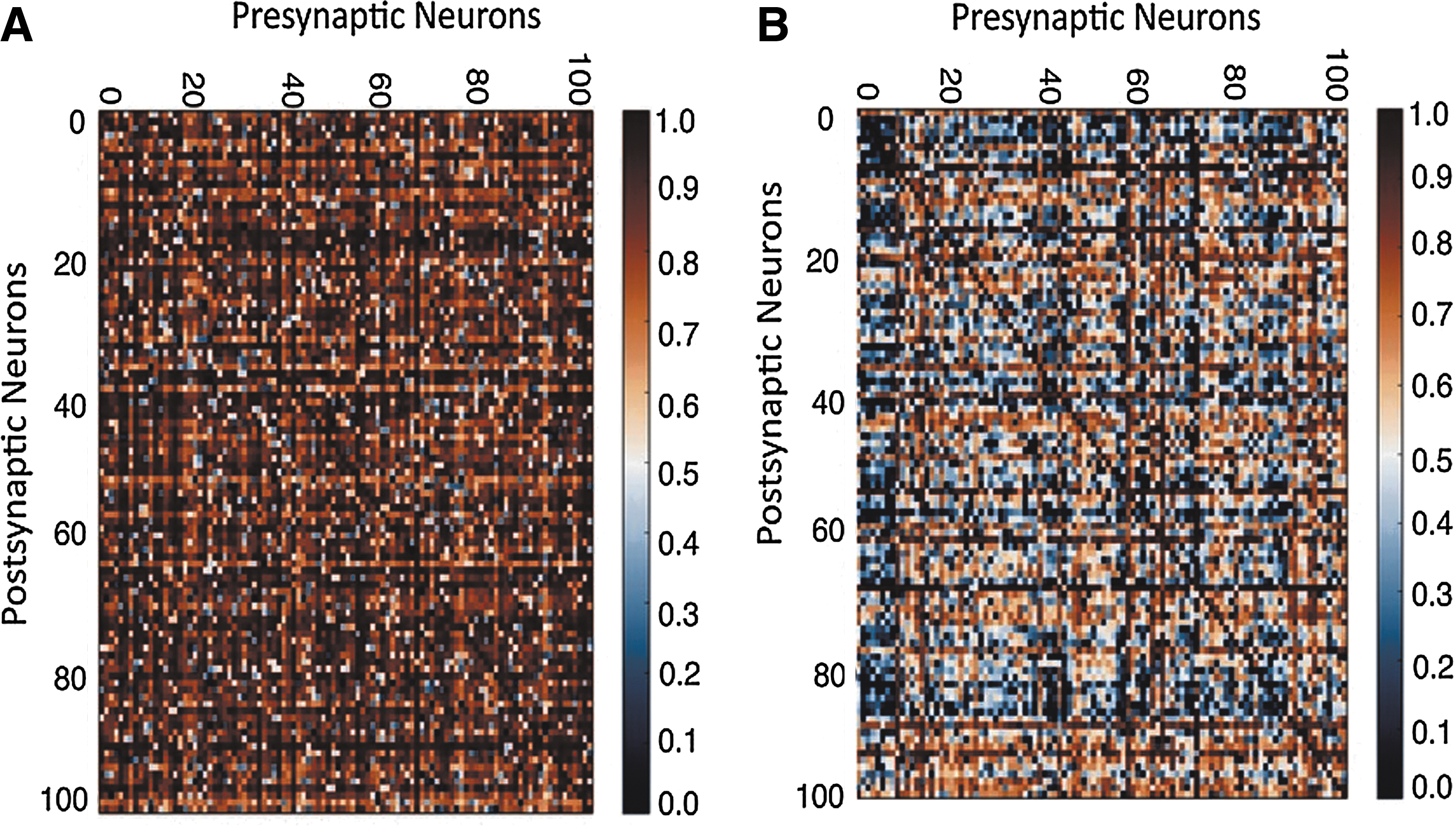
Next, we investigate how systematic potentiation and depression of local excitatory synaptic weights w_tc may modify local connectivity between pre- and postsynaptic neuron pairs in a node model in the presence and absence of brain-state dependent input. To address this, we access local cortical SC by calculating synaptic weights in the presence and absence of rhythmic input and STDP (Fig. 5). Initially, presynaptic and postsynaptic neurons are connected in an all-to-all fashion. Hence, all synaptic weights are 1. Without rhythmicity in the input, that is, if STDP is random, weight changes between pre-post are also random and show up in the result (Fig. 5A). This is intuitively correct, as plasticity in this scenario is less prevalent and any change in weights between pairs, that is, potentiation or depression, due to the realization of STDP is rather random. In contrast, with a rhythmic background input, structure emerges in the layout of connectivity between pre- and postsynaptic neurons and local clustering is observed (Fig. 5B). The clustering of weights plays an important role in constraining local area node dynamics as shown in computational (Voges and Perrinet, 2012) and experimental work using two-photon calcium imaging in vivo and multiple whole-cell recordings in vitro in rodents' primary visual cortex (Ko et al., 2013). To obtain a systematic insight about local node model behavior under various conditions on a longer time scale, activity of the node network is simulated for 60 sec. Resulting summed membrane potential activity, that is, LFP and corresponding time frequency plots are displayed in Figure 6. The rhythmic input leads to an oscillation in the population-firing rate, as otherwise is not possible when relying only on the intrinsic network parameters used for the spiking node model. Integrated spontaneous activity shows intermittent low-frequency (3–8 Hz) locking (Fig. 6B). With a rhythmic input, LFP network activity exhibits network oscillations in the alpha frequency range (Fig. 6C). For a rhythmic input with STDP network, activity is shown in a time frequency plot in Figure 6D demonstrating continuous periodic oscillations and phase locking to the alpha frequency band.

FIG. 6.

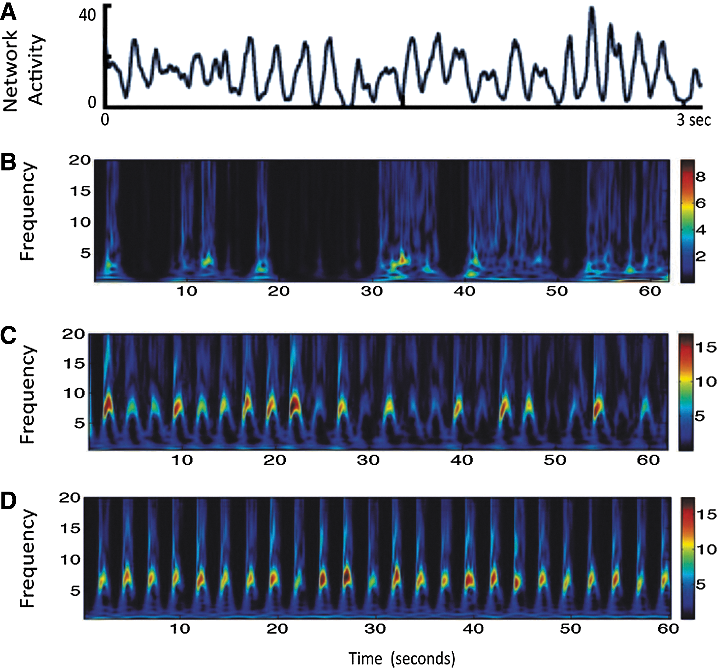
Spiking IF neuron model network activity is simulated for 60 sec. It exhibits band-restricted oscillations in the alpha frequency range. (A) Simulated spontaneous local field potential (LFP) activity (10 ms sliding window) in the absence of rhythmic input and STDP (3 sec) exhibits oscillations in the 8–12 Hz frequency range. (B) Time-frequency plot for integrated network activity is shown for the entire duration of spontaneous activity with intermittent locking to alpha and also low-frequency scale. (C) Time-frequency plot for integrated network activity with rhythmic input displays periodic 10 Hz oscillations with an intermittent decrease in power. (D) After enabling STDP band-specific power in local node increases and frequency locks to the rhythmic modulation of phase of the feed-forward drive (intrinsic network parameters are held at the same values as displayed in Table 2). Color images available online at www.liebertpub.com/brain

Analytical approximation of synaptic weight change in time due to STDP in the cortical model

Rates of the presynaptic spike trains are approximated by a continuous sinusoid. Hence, feed-forward input to a cortical region is described as an inhomogeneous Poisson process: \documentclass{aastex}\usepackage{amsbsy}\usepackage{amsfonts}\usepackage{amssymb}\usepackage{bm}\usepackage{mathrsfs}\usepackage{pifont}\usepackage{stmaryrd}\usepackage{textcomp}\usepackage{portland, xspace}\usepackage{amsmath, amsxtra}\pagestyle{empty}\DeclareMathSizes{10}{9}{7}{6}\begin{document} \begin{align*}I ( t ) = r ( 1 - \cos ( {\,ft} ) ) \tag{9}\end{align*} \end{document}

where f is the angular frequency, and r is the peak firing rate. The spikes in the output are delivered as series of delta pulses of the following form: \documentclass{aastex}\usepackage{amsbsy}\usepackage{amsfonts}\usepackage{amssymb}\usepackage{bm}\usepackage{mathrsfs}\usepackage{pifont}\usepackage{stmaryrd}\usepackage{textcomp}\usepackage{portland, xspace}\usepackage{amsmath, amsxtra}\pagestyle{empty}\DeclareMathSizes{10}{9}{7}{6}\begin{document} \begin{align*}J ( t ) = \mathop\sum_k \delta ( t - \frac { 2k \pi + \psi } { f } ) \tag { 10 } \end{align*} \end{document}

where ψ is the phase offset of the output spikes. The phase distribution of the delta function reflects the assumption of phase locking in population spikes. We have verified numerically the behavior that is similar for any moderately peaked unimodal distributions.

In order to compute a correlation between input oscillations and output pulses, we perform the following integration: \documentclass{aastex}\usepackage{amsbsy}\usepackage{amsfonts}\usepackage{amssymb}\usepackage{bm}\usepackage{mathrsfs}\usepackage{pifont}\usepackage{stmaryrd}\usepackage{textcomp}\usepackage{portland, xspace}\usepackage{amsmath, amsxtra}\pagestyle{empty}\DeclareMathSizes{10}{9}{7}{6}\begin{document} \begin{align*}D ( J ) = \frac { fr } { 2 \pi } \int \limits_ { - \infty } ^ { \infty } [ 1 - \cos ( { \,ft } ) ] \delta \left( t - \frac { \psi } { f } - \Delta t \right) dt \tag { 11 } \end{align*} \end{document}

where Δt is the difference in the spike times between t_pre −t_post . In other words, this reflects the STDP time window. The correlation integral is further simplified: \documentclass{aastex}\usepackage{amsbsy}\usepackage{amsfonts}\usepackage{amssymb}\usepackage{bm}\usepackage{mathrsfs}\usepackage{pifont}\usepackage{stmaryrd}\usepackage{textcomp}\usepackage{portland, xspace}\usepackage{amsmath, amsxtra}\pagestyle{empty}\DeclareMathSizes{10}{9}{7}{6}\begin{document} \begin{align*}D ( J ) = \frac { fr } { 2 \pi } [ 1 - \cos ( \psi - fJ ) ] \tag { 12 } \end{align*} \end{document}

To obtain the change of weight w(t) over time, we make use of D(J) in Eq. (12) to write it as a function of input phase of oscillations: \documentclass{aastex}\usepackage{amsbsy}\usepackage{amsfonts}\usepackage{amssymb}\usepackage{bm}\usepackage{mathrsfs}\usepackage{pifont}\usepackage{stmaryrd}\usepackage{textcomp}\usepackage{portland, xspace}\usepackage{amsmath, amsxtra}\pagestyle{empty}\DeclareMathSizes{10}{9}{7}{6}\begin{document} \begin{align*} \frac { dw } { dt } = w_ { \max } \int \limits_ {- \infty } ^ { \infty } F ( J ) D ( J ) dJ \tag { 13 } \end{align*} \end{document}

Now, we can carry out an explicit integration in the subsequent steps, \documentclass{aastex}\usepackage{amsbsy}\usepackage{amsfonts}\usepackage{amssymb}\usepackage{bm}\usepackage{mathrsfs}\usepackage{pifont}\usepackage{stmaryrd}\usepackage{textcomp}\usepackage{portland, xspace}\usepackage{amsmath, amsxtra}\pagestyle{empty}\DeclareMathSizes{10}{9}{7}{6}\begin{document} \begin{align*}{dw \over dt} & = {frw_{ \max} \over 2 \pi} \left[ \int \limits_{0}^{ \infty}A_{ + }e^{ - {J \over \tau_ + }} [ 1 - \cos ( \psi - fJ ) ] dJ \right. \\ & \quad\left. - \int \limits_{- \infty}^{0}A_{ - }e^{J \over { \tau_ - }} [ 1 - \cos ( \psi - fJ) ] dJ \right] \\ {dw \over dt} & = {frw_{ \max} \over 2 \pi} \left[ \int \limits_{0}^{ \infty}A_{ + }e^{ - {J \over \tau_ + }} dJ - \int \limits_{ \infty}^{0} A_{ + }e^{ - {J \over \tau_ + }} \cos ( \psi - fJ ) dJ \right. \\ & \quad\left.- \int \limits_{ - \infty}^{0} A_{ - }e^{{J \over \tau_ - }} dJ + \int \limits_{ - \infty}^{0} A_{ - }e^{J \over \tau_ - } \tau_{-} \cos ( \psi - fJ) dJ \ \right] \\ & & ( 14 ) \end{align*} \end{document}

We can further simplify Eq. (14) as follows: \documentclass{aastex}\usepackage{amsbsy}\usepackage{amsfonts}\usepackage{amssymb}\usepackage{bm}\usepackage{mathrsfs}\usepackage{pifont}\usepackage{stmaryrd}\usepackage{textcomp}\usepackage{portland, xspace}\usepackage{amsmath, amsxtra}\pagestyle{empty}\DeclareMathSizes{10}{9}{7}{6}\begin{document} \begin{align*}\frac {dw}{dt} & = \frac {frw_{ \max}}{2 \pi} \left[ \frac{A_{ - }}{\frac{1}{\tau_{ - }^2} + f^2} \left( \frac {\cos \psi}{\tau_{-}} - f \sin \psi \right) \right. \\ &\quad \left. - \frac {A_+}{{1 \over \tau_{ + }^2} + f^2} \left( \frac{\cos \psi}{\tau_ +} + f \sin \psi \right) - A_{ - } \tau_{ - } + A_{ +} \tau_{ + } \right] \tag{15}\end{align*} \end{document}

Eq. (15) describes how—in the presence of plasticity—the synaptic weights w(t) evolve in time as a function of frequency of input oscillation f, input modulatory phase ψ, synaptic plasticity time constants τ ₊, τ ₋, or the ratio of depotentiation-potentiation \documentclass{aastex}\usepackage{amsbsy}\usepackage{amsfonts}\usepackage{amssymb}\usepackage{bm}\usepackage{mathrsfs}\usepackage{pifont}\usepackage{stmaryrd}\usepackage{textcomp}\usepackage{portland, xspace}\usepackage{amsmath, amsxtra}\pagestyle{empty}\DeclareMathSizes{10}{9}{7}{6}\begin{document}$$ \frac { A_ + } { A_ { - } } $$ \end{document} . We simulate a spiking network of neurons numerically with the oscillation frequency f being 10 Hz, the STDP time constants being equal and set to 20 ms, A ₊ being 0.01, and the STDP ratio being held in the range of [1.4–1.9].

Alteration of FC and Dynamic Landscape Due to Locally Restricted Plasticity

In this section, we test the hypothesis that a change in local node spiking dynamics due to altered SC between thalamus and a single cortical node has an impact on adjacent as well as on distant node correlations. Here, we systematically explore how the local plasticity alters the global repertoire. How the local plastic change translates into global functional and structural restructuring is illustrated schematically in Figure 7. In a previous work, we have reported learning-related changes in empirical rs-FC as reflected by the difference in the imaginary component of coherence before and after learning (Freyer et al., 2012a). Imaginary coherence reflects the functional correlation between the areas from which EEG waveforms are recorded on the scalp, avoiding effects of volume conduction. To access the FC before and after plasticity, we simulate a global brain model consisting of six brain areas connected via long-range SC. Therefore, it will have an impact on global functional correlations across brain areas. As a first step, in the absence of plastic changes, we obtain a bifurcation diagram by varying the global scaling input parameter G to six brain regions using both spiking and the DMF model. A comparison of global dynamics between the spiking and mean field description is plotted in Figure 8A. Qualitatively, both models exhibit multistability in a range of global coupling parameter values. As shown in Figure 8B using the DMF model, a value of global scaling parameter G>4.0 network destabilizes and the selected six cortical regions exhibit high firing rates. For the color-coded representative points, we obtain population firing rates from the six selected brain regions. They display low asynchronous population firing rates around 3–4 Hz and high firing rates around 50–60 Hz for stronger scaling parameter values. In between, we obtain multi stability in the global model (Fig. 8C). Next, we introduced brain state-driven feed-forward thalamic input to a cortical node and modified the synaptic weights within that node in accordance with our synaptic plasticity rule. Using plasticity in the node model, first we estimate local coherence from resulting spike times and subsequently using local coherence to estimate a free energy function. The degree of synchronization of the spiking neurons in the local cortical area is measured by order parameter \documentclass{aastex}\usepackage{amsbsy}\usepackage{amsfonts}\usepackage{amssymb}\usepackage{bm}\usepackage{mathrsfs}\usepackage{pifont}\usepackage{stmaryrd}\usepackage{textcomp}\usepackage{portland, xspace}\usepackage{amsmath, amsxtra}\pagestyle{empty}\DeclareMathSizes{10}{9}{7}{6}\begin{document}$$R ( t ) = \big| \frac { 1 } { N } \sum_k e^ { i \theta_k } \big|$$ \end{document} , where \documentclass{aastex}\usepackage{amsbsy}\usepackage{amsfonts}\usepackage{amssymb}\usepackage{bm}\usepackage{mathrsfs}\usepackage{pifont}\usepackage{stmaryrd}\usepackage{textcomp}\usepackage{portland, xspace}\usepackage{amsmath, amsxtra}\pagestyle{empty}\DeclareMathSizes{10}{9}{7}{6}\begin{document}$$\theta_k ( t ) = 2 \pi ( t - t_k^m ) / ( t_{m + 1}^k - t_m^k )$$ \end{document} is the phase of the k^th neuron at time t between m^th and (m+1)^th spike times. For asynchronous systems, R=0 and R=1 for a perfectly synchronous system; while for intermediate values, groups of neurons are partially synchronized. The probability distribution function (PDF) of the order parameter R(t) is estimated by observing its long time averaged trajectory, and the associated energy profile is given by F(R)=−log P(R)_, where P is the probability density of R. Local landscape modifications due to synaptic plasticity as well as global change in dynamics as a function of global input scaling parameter G are plotted in Figure 9A and B. We find that in addition to noise, synaptic plasticity also systematically drives the mean firing activity between various cortical states (a low as well as high firing activity as a function of global scaling parameter). In the absence of plasticity, thalamic noise input drives the local cortical brain area from low firing asynchronous activity to high synchronous firing activity (Fig. 9B). In the presence of STDP in the local cortical pool, the jumps between minima are driven by the macroscopic evolution of local synaptic plasticity via synaptic weight updates w(t). This constrains the mean firing rate of populations when they are linked via global coupling as shown in Figure 9A. Now, globally they achieve a partially synchronous oscillatory state, thereby elevating firing rates of a substantial number of connected cortical regions for low coupling G values. For the high global input scaling values of G, they exhibit very high synchronous firing activity. Figure 10 shows the SC distance and capacity matrices reflecting the connection lengths and strengths of fiber tracts connecting these brain regions. As a toy data set, we chose the bilateral areas primary somatosensory area S1 (where plasticity is implemented), primary motor area M1, and thalamus. Realistic SC was taken from TVB database. Next, we look at global FC before and after plasticity-related change in the mean firing activity of relevant cortical pools. We compute FC between the six areas before and after plastic change as shown in Figure 10C–E. FC between distantly connected areas are rather weak as shown in the correlation map, while the FC between adjacent areas are relatively stronger. FC is determined by the connection strengths between regions displayed in Figure 10B. After local plastic alterations in right S1, FC show enhancement between adjacent as well as between distantly connected areas in the thalamus, S1, and M1, respectively (Fig. 10C, D). This demonstrates an important link between local structure and global FC. After plastic alterations in local SC, there is also a high number of de-correlated brain areas as can be seen in Figure 10D. The change in rs-FC may indicate specific switches in brain states. This can be understood by studying slow (<0.1 Hz) oscillations (Biswal et al., 1995) commonly thought to signal general changes in network excitability (Honey et al., 2007), whereas oscillations on a faster timescale (8–12 Hz) may be more well suited to more specific information flow between areas (Honey et al., 2012). Interactions between relevant network areas on a faster time scale can be examined by looking at the pair-wise LFP network activity. If two areas were highly synchronized, the coherence measure would yield values close to 1, while in the opposite scenario values would stay close to zero. One could also look at the spectrogram by filtering the LFP network activity and obtain a measure of the dominant band specific activity as displayed in Figure 6. Next, we look at the spontaneous activity recorded from a single human subject EEG from somato-sensory cortical regions versus simulated neuronal signals filtered at the rate of EEG. For cortical area S1, we can obtain qualitatively similar spontaneous activity in the range of (8–10 Hz frequency band) in our network model (with local parameters fixed w_EI =w_IE =w_II =1) by adjusting feed-forward thalamic weights (an important control parameter in the plasticity model) using updates according to the synaptic plasticity rule or in the absence of plasticity purely driven by thalamic noisy input. In Figure 11A and B, we plotted spontaneous alpha-like activity and the corresponding spectrogram in terms of signal amplitude and frequency power. In Figure 11C and D, amplitude waveform from simulated signal in the bandwidth of (8–15 Hz) shows remarkable concordance with empirical EEG signals. Finally, we look at the power in the signal bandwidth of 10 Hz (Fig. 11E) which shows that fluctuations are organized into two specific modes (low and high power fluctuations in the both model and empirical signal) as previously reported in Freyer and colleagues (2011). As hypothesized by Freyer and associates (2011), we have just verified that the transition from cortical low to high power resting-state activity is influenced by thalamic noisy input.

FIG. 7.

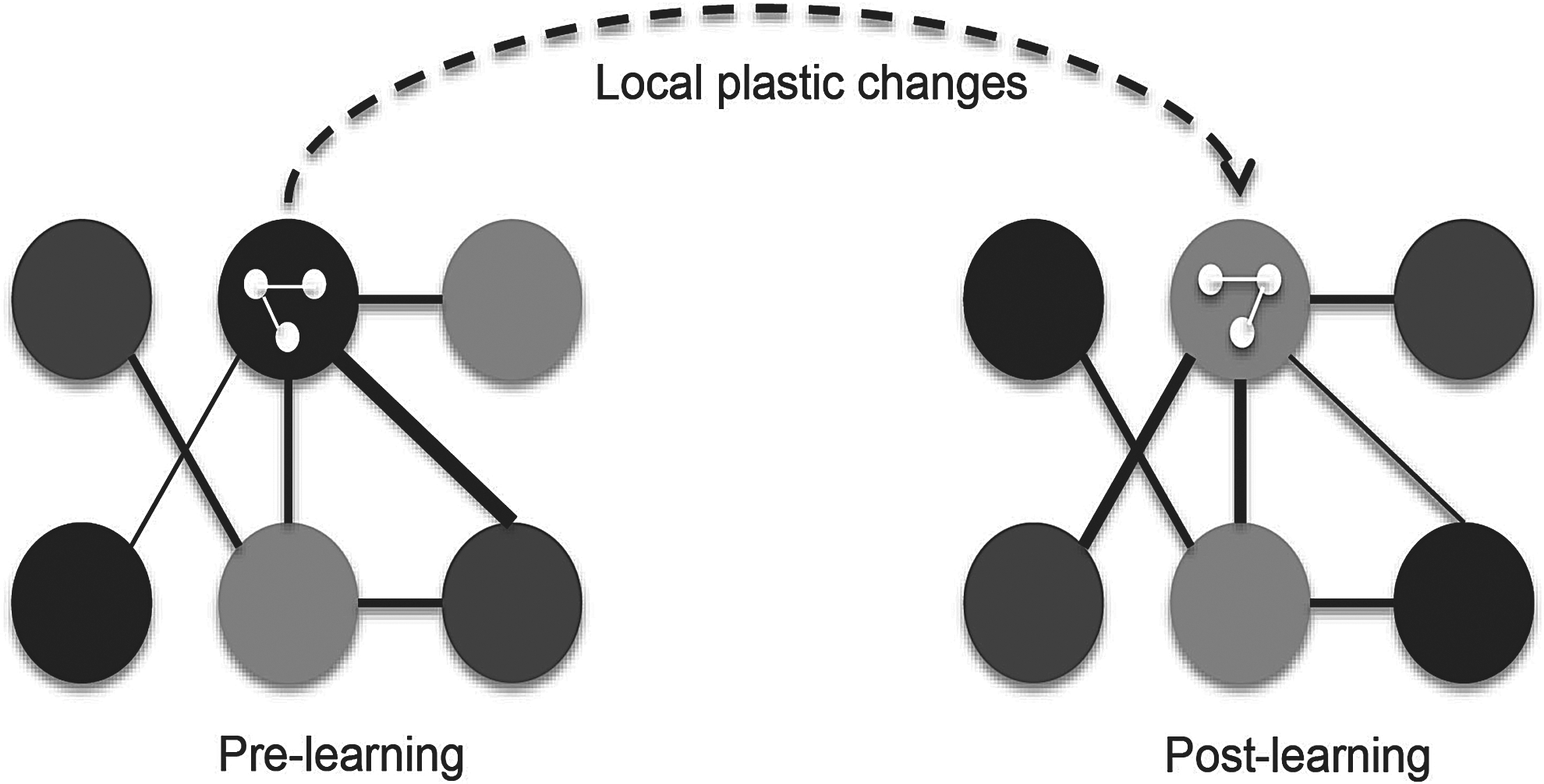
SC between six simulated cortical nodes and changes in global SC due to local plastic effects. Upper panel: A functional network is represented by six interconnected neural populations or regions represented by six large circles. Each node comprises the same number of excitatory and inhibitory neurons connected via recurrent connections within regions, represented by three small white pellets connected by white lines in the central-upper large pellet. SC is illustrated by black lines connecting the regions. Resting-state functional connectivity (rs-FC), that is, degree of correlation, is represented by the gray scales in the six regions, with similar scales indicating a high degree of coherence. After learning, as the dashed arrow indicates, local plasticity within a region changes. This is exemplified by the change of white local connections. Postlearning local changes are paralleled by global changes in FC, illustrated here by the reconfiguration of the connecting lines and the gray colors among the six regions.

FIG. 8.

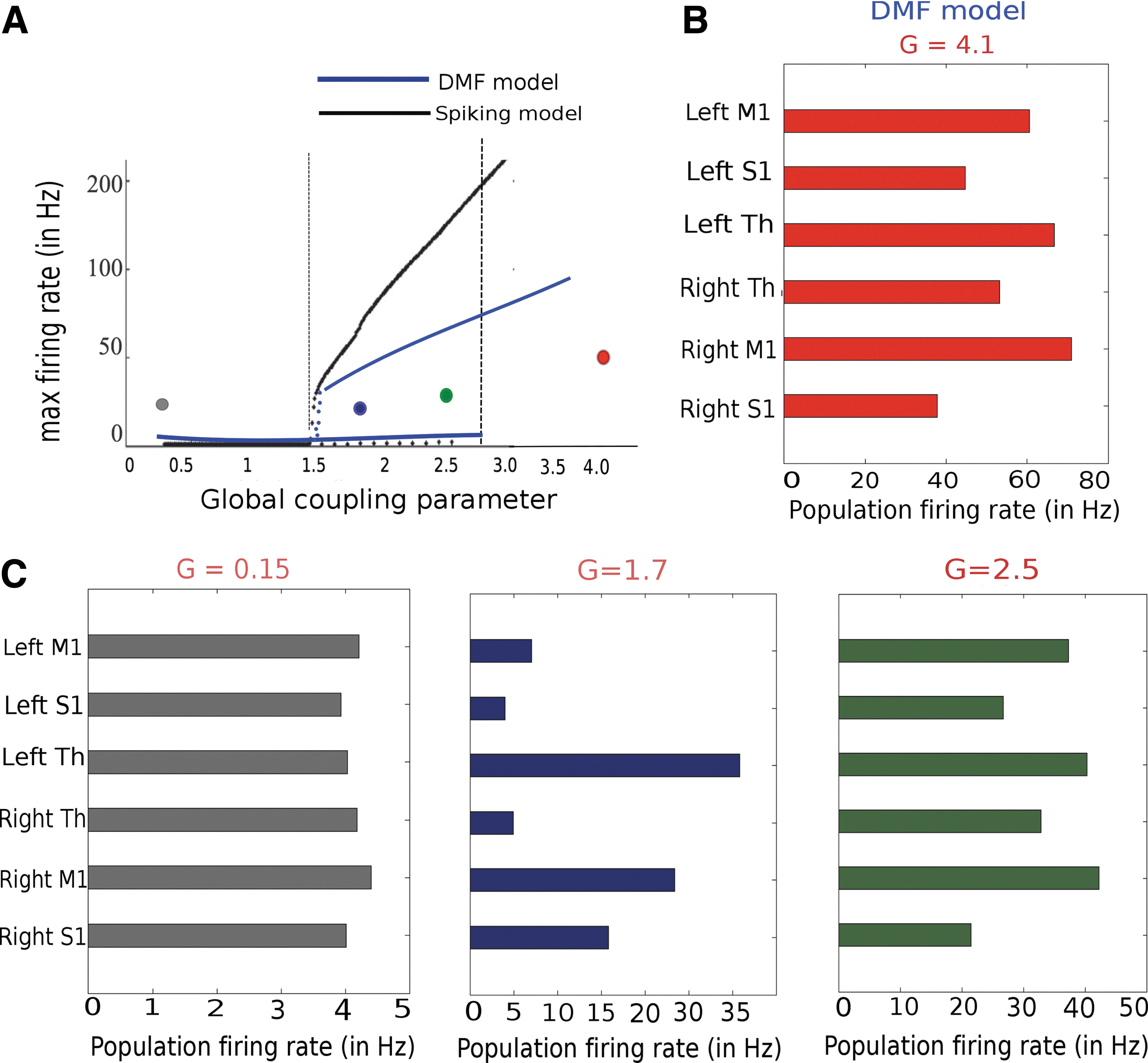
Bifurcation diagrams of the full spiking model and the reduced dynamic mean field (DMF) model. (A) Mean-field analyses of the attractor landscape of the spiking network (black) and the reduced DMF model (blue) yields maximum firing rate activity among all nodes as a function of a single free parameter global coupling strength G. The models incorporate a realistic SC matrix composed of 74 regions obtained from a TVB database. Solid lines (black, blue) indicate the stable branches in the bifurcation diagram. In both cases, depending on the coupling strength G and the initial conditions, the network converges to one of three possible dynamical regimens. (B) Firing rate (red) for a representative point as shown in red in (A) using the DMF model and a value of G>4.0. For this value, the network destabilizes and relevant cortical regions exhibit high firing rates. (C) Firing rates generated by the spiking neuron model for three representative points as shown in gray, blue, and green in (A). A selection of six cortical and subcortical regions of interest is depicted. For low values of G, the network converges to a single stable state of low firing activity, that is, the spontaneous state. For increasing values of G, new stable states of high activity along with the spontaneous state coexist. For even larger values of G, the spontaneous state becomes unstable. Color images available online at www.liebertpub.com/brain

FIG. 9.

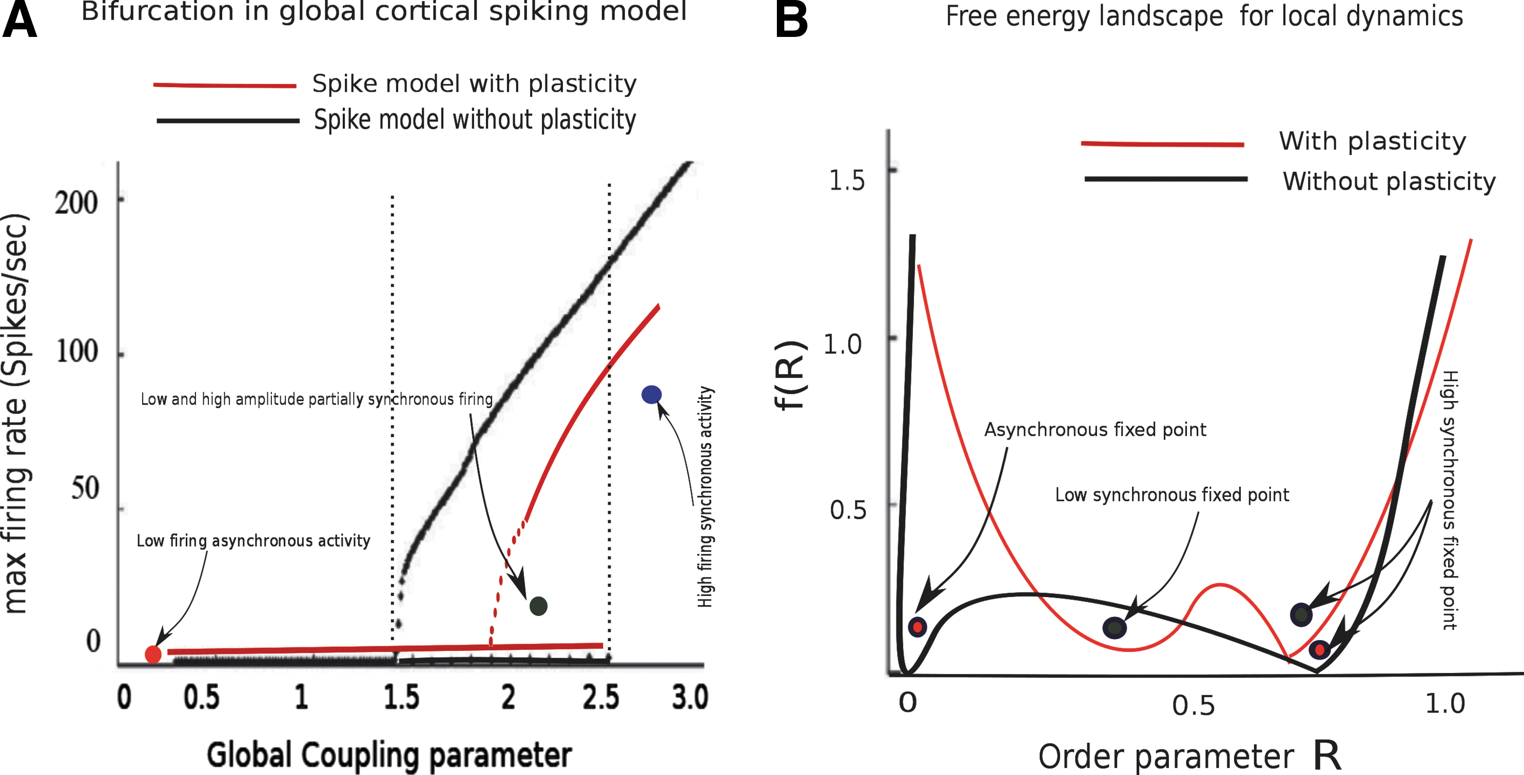
Bifurcation in the global cortical model and relationship with local area dynamics unfolded on a free energy landscape with STDP. (A) Mean-field analyses of the attractor landscape of the global cortical spiking network as a function of a single free parameter global coupling strength (G) that regulates the amount of the global input current. Black: without STDP. Red: with STDP in locally restricted (thalamus-S1). Each point residing on the solid lines (black, red, indicating the stable branches in the bifurcation diagram) represents the maximum firing rate activity among all relevant cortical nodes (here 6 nodes). In both cases, depending on the coupling strength (G) and the initial conditions, the network converges to one of three possible dynamical regimens: 1) a single fixed point regime - the region is indicated by a red point - with asynchronous low firing (without STDP) or medium firing activity (with STDP); 2) a regime of low as well as high firing activity with partial synchrony (multistability) indicated by a representative point in green and; 3) a regime with high firing synchronous activity indicated by a representative point in blue. (B) STDP alters correlations between left thalamus and S1. Inter-node correlations are assessed by a free energy diagram. The free energy function is plotted in black solid line (without STDP) and in red solid line (with STDP). A change was found in local fixed-point dynamics as a function of synchrony, i.e. order parameter R, in left S1. The energy landscape indicates modified output dynamics of local brain area S1 mediated by feed-forward input oscillation and synaptic plasticity. Subsequently this change modifies the resulting global activity of connected brain areas as indicated by altered maximum firing rates of the cortical pools. Without STDP, the energy function f(R) exhibits two minima at phases R=0 (asynchronous fixed point dynamics) and R=0.85 (synchronous dynamics). The local minima are separated by a saddle located at R=0.3. Jumps between minima are mainly carried out by noise driven transitions (when isolated from global input). With STDP, f(R) has two minima. In this case the asynchronous fixed point is substituted by a partially low synchronous fixed-point dynamics at phase R=0.35 and the high synchronous fixed point at phase R=0.82. They are also separated by a saddle at R=0.56, however there is noticeable difference in the depth of the energy landscape compared to the case without STDP. Color images available online at www.liebertpub.com/brain

FIG. 10.

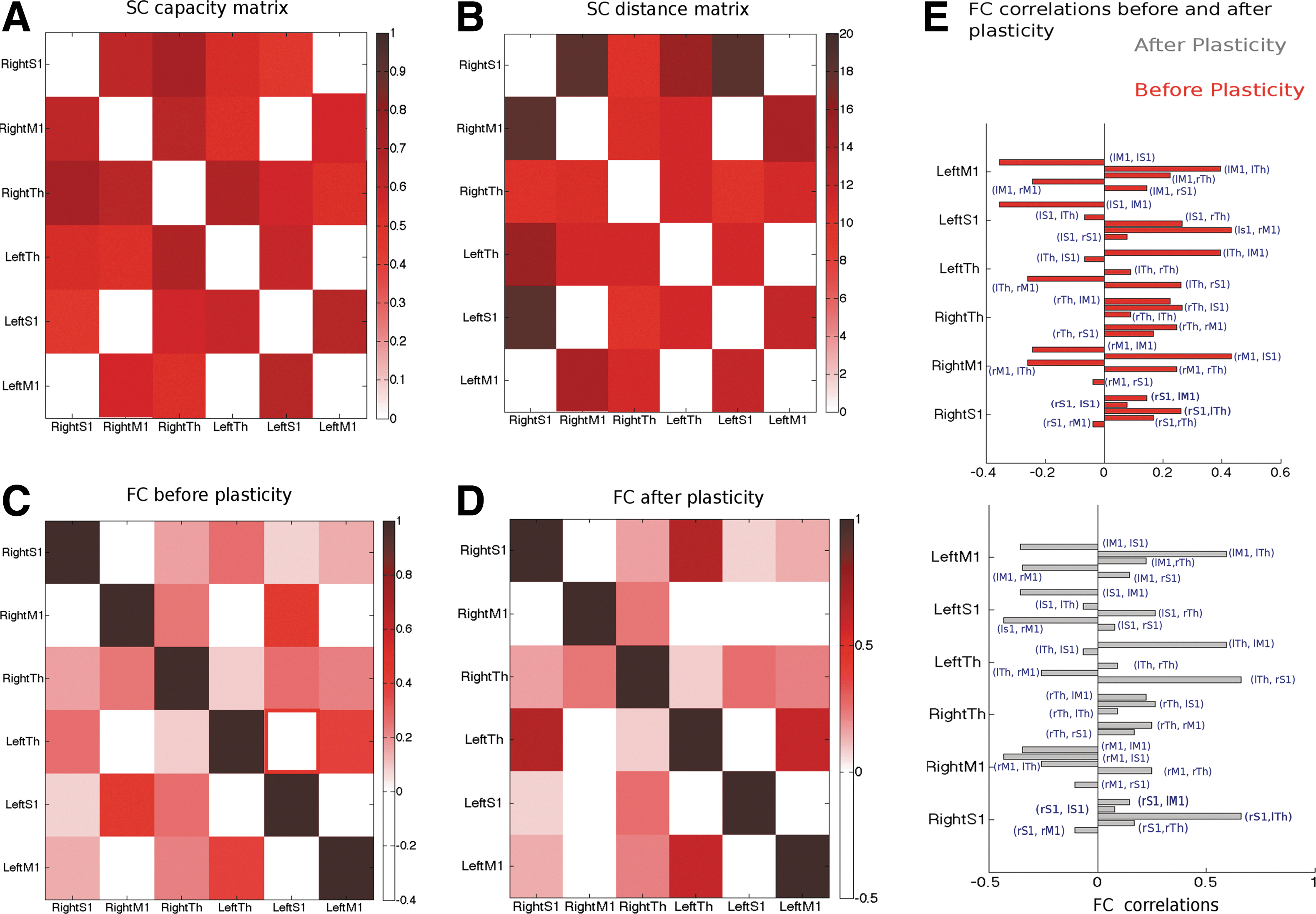
Realistic SC and simulated FC between salient brain regions. (A) SC capacity matrix indicating connection strengths and (B) SC distance matrix indicating fiber tract lengths between six cortical regions comprising bilateral primary somatosensory areas (right, left S1), primary motor areas (right, left M1), and thalamus (left, right Th). The color bar indicates the weights and the edge lengths between corresponding cortical areas. Simulated brain nodes (IF neurons) and FC accessed computing pair-wise correlations before and after structural connectivity change between left S1-left Th. The FC matrices represent six brain areas corresponding to regions in the SC matrices above. (C) Functional correlation map shows weak or zero correlations between structurally not connected areas. (D) Correlation map shows changed FC; for example, enhanced correlations between some areas that were weakly correlated before local plasticity, for example, right S1-M1. Self-correlation between same areas that is always 1 is represented by the diagonal in the correlation map and is set to zero. (E) In the top (red) and bottom panel (gray), FC (before and after plasticity) are shown with a bar diagram (corresponding region pairs are labeled). Increases, decreases, and no alterations in positive as well as negative correlations between cortical regions before (red) and after (gray) plasticity can be seen. Color images available online at www.liebertpub.com/brain

FIG. 11.

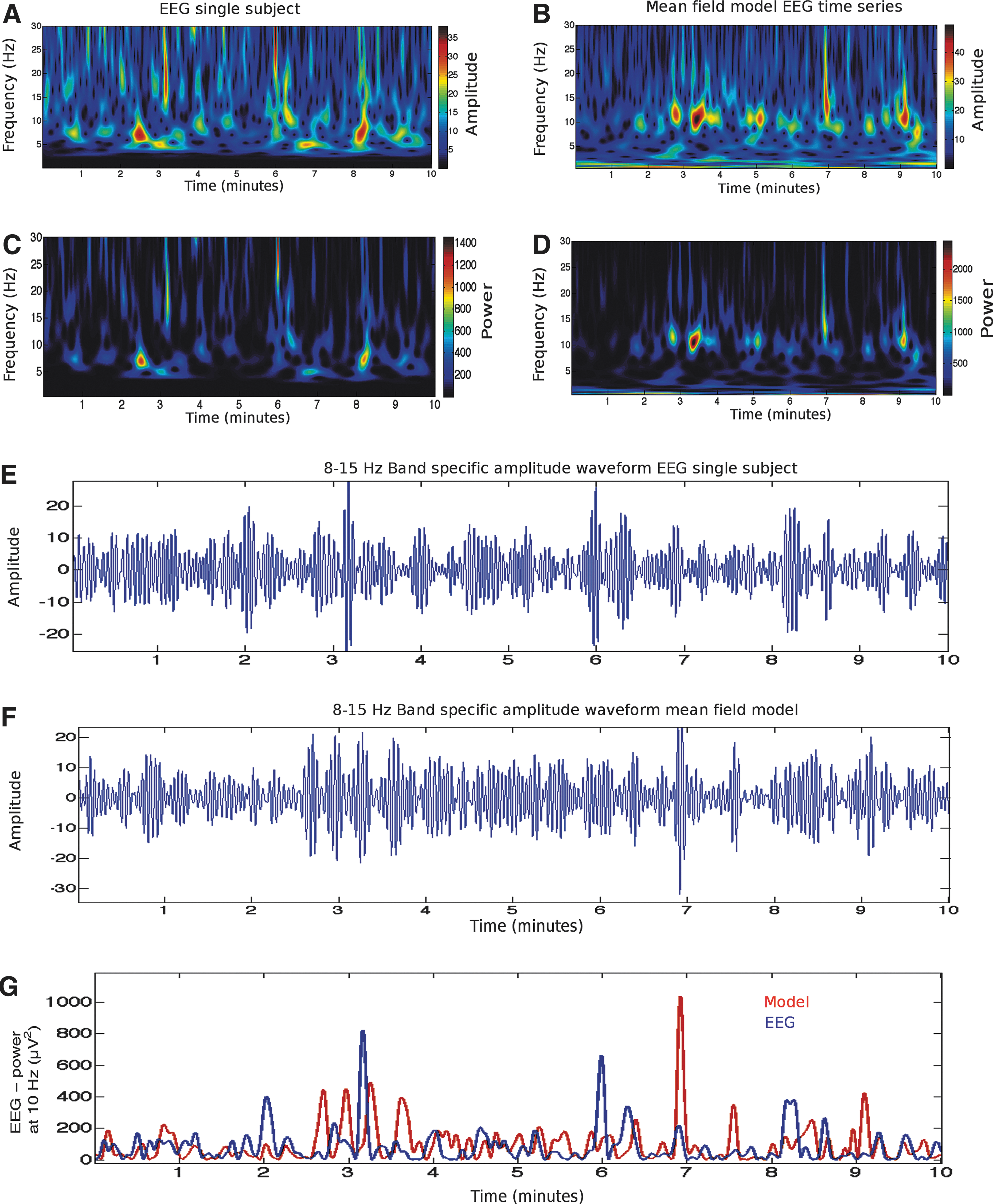
Time series analysis of experimental electroencephalography (EEG) data and the output of a mean field model. (A) Spectrogram of the EEG of a single subject. The signal comes from channel CP3 in the EEG field map, which is located over the somatosensory cortex. EEG data from Freyer and coworkers (2012a, 2013). (B) Spectrogram of the signal output of the mean field model at cortical area S1. The model is driven by thalamic noise in the absence of state-dependent input and synaptic plasticity with intrinsic recurrent network parameters as described in single brain area spiking model. For (A) and (B), the colorbar indicates the amplitude of the signal. (C, D) Time series signal power of the experimental and simulated data. High power is found in the alpha range. (E, F) Amplitude waveform for EEG data as well for the model output in the alpha frequency band. Waxing and waning of alpha power corresponding to low and high amplitude bursts can be observed. (G) Signal power at 10 Hz is plotted over time for experimental and simulated data. Switching of power from low to high values can be seen—indicating multistability that in the model is driven by thalamic noise coming from feed-forward glutamatergic synapses. Color images available online at www.liebertpub.com/brain

Analytical approximation of activity covariance in the global cortical model

In order to estimate the network activity and statistics, we use statistical first- and second-order moments equations to approximate the deterministic gating equations in the DMF model as displayed in Eq. (6). We first express stochastic differential equations in terms of their first and second moments of the distribution of the gating variable: \documentclass{aastex}\usepackage{amsbsy}\usepackage{amsfonts}\usepackage{amssymb}\usepackage{bm}\usepackage{mathrsfs}\usepackage{pifont}\usepackage{stmaryrd}\usepackage{textcomp}\usepackage{portland, xspace}\usepackage{amsmath, amsxtra}\pagestyle{empty}\DeclareMathSizes{10}{9}{7}{6}\begin{document}$$\lambda^m_a$$ \end{document} mean gating variable of local neural population (m=E or 1) of the cortical area a. We also define a covariance matrix between two distinct neural populations {a, b} and {m, n} reflecting arbitrary cortical areas as \documentclass{aastex}\usepackage{amsbsy}\usepackage{amsfonts}\usepackage{amssymb}\usepackage{bm}\usepackage{mathrsfs}\usepackage{pifont}\usepackage{stmaryrd}\usepackage{textcomp}\usepackage{portland, xspace}\usepackage{amsmath, amsxtra}\pagestyle{empty}\DeclareMathSizes{10}{9}{7}{6}\begin{document}$$p_{ab}^{mn}$$ \end{document} . Now, we can write the statistical moments as follows: \documentclass{aastex}\usepackage{amsbsy}\usepackage{amsfonts}\usepackage{amssymb}\usepackage{bm}\usepackage{mathrsfs}\usepackage{pifont}\usepackage{stmaryrd}\usepackage{textcomp}\usepackage{portland, xspace}\usepackage{amsmath, amsxtra}\pagestyle{empty}\DeclareMathSizes{10}{9}{7}{6}\begin{document} \begin{align*}\lambda_i^m = \langle E_i^m \rangle \tag{16}\end{align*} \end{document} \documentclass{aastex}\usepackage{amsbsy}\usepackage{amsfonts}\usepackage{amssymb}\usepackage{bm}\usepackage{mathrsfs}\usepackage{pifont}\usepackage{stmaryrd}\usepackage{textcomp}\usepackage{portland, xspace}\usepackage{amsmath, amsxtra}\pagestyle{empty}\DeclareMathSizes{10}{9}{7}{6}\begin{document} \begin{align*}p_{ab}^{mn} ( t ) = \langle [ E_a^m - \lambda_a^m ] [ E_b^n - \lambda_b^n ] \rangle \tag{17}\end{align*} \end{document}

where <.> expectation values over many realizations. In the vector field form, synaptic gating variable equations are expressed as \documentclass{aastex}\usepackage{amsbsy}\usepackage{amsfonts}\usepackage{amssymb}\usepackage{bm}\usepackage{mathrsfs}\usepackage{pifont}\usepackage{stmaryrd}\usepackage{textcomp}\usepackage{portland, xspace}\usepackage{amsmath, amsxtra}\pagestyle{empty}\DeclareMathSizes{10}{9}{7}{6}\begin{document} \begin{align*} \frac { d } { dt } ( \vec { E } ^ { exc } ) & = ( F^ { exc } ( \vec { E } ^ { exc } , \vec { E } ^ { inh } ) ) \\ \frac { d } { dt } ( \vec { E } ^ { inh } ) & = ( F^{ inh } ( \vec { E } ^ { exc } , \vec { E } ^ { inh } ) ) & \qquad\qquad(18) \end{align*} \end{document}

where for excitatory and inhibitory populations Eq. (18) can be expressed as (simply following as defined in Eq. (6) deterministic dynamics of SDE) follows: \documentclass{aastex}\usepackage{amsbsy}\usepackage{amsfonts}\usepackage{amssymb}\usepackage{bm}\usepackage{mathrsfs}\usepackage{pifont}\usepackage{stmaryrd}\usepackage{textcomp}\usepackage{portland, xspace}\usepackage{amsmath, amsxtra}\pagestyle{empty}\DeclareMathSizes{10}{9}{7}{6}\begin{document} \begin{align*} & \vec { E } = \ { \vec { E } ^ { exc } , \vec { E} ^ { inh } \ } = \ { E_1^ { exc } , \ldots \ldots. \,, E_N^ { exc} , E_1^ { inh } , \ldots \ldots. \,, E_N^ { inh } \ } \\ & F_n^ { exc } = - \frac { E_n^ { exc } } { \tau_ { exc } } + ( 1 - E_n^ { exc } ) \gamma r^ { exc } ( I_n^ { exc } ) \\& F_ { n } ^ { inh }= - \frac { E_n^ { inh } } { \tau_ { inh } } + r^ { inh } ( I_n^{ exc } ) \qquad { \rm for } \ \forall n = 1 , \ldots \ldots , N &( 19 ) \end{align*} \end{document}

Since we are dealing with a deterministic system, a Taylor expansion of the vector field of gating variable \documentclass{aastex}\usepackage{amsbsy}\usepackage{amsfonts}\usepackage{amssymb}\usepackage{bm}\usepackage{mathrsfs}\usepackage{pifont}\usepackage{stmaryrd}\usepackage{textcomp}\usepackage{portland, xspace}\usepackage{amsmath, amsxtra}\pagestyle{empty}\DeclareMathSizes{10}{9}{7}{6}\begin{document}$$\vec{E}$$ \end{document} about moments \documentclass{aastex}\usepackage{amsbsy}\usepackage{amsfonts}\usepackage{amssymb}\usepackage{bm}\usepackage{mathrsfs}\usepackage{pifont}\usepackage{stmaryrd}\usepackage{textcomp}\usepackage{portland, xspace}\usepackage{amsmath, amsxtra}\pagestyle{empty}\DeclareMathSizes{10}{9}{7}{6}\begin{document}$$\vec{ \lambda} = \langle \vec{E} \rangle$$ \end{document} up to only the first-order terms, this allows us to write: \documentclass{aastex}\usepackage{amsbsy}\usepackage{amsfonts}\usepackage{amssymb}\usepackage{bm}\usepackage{mathrsfs}\usepackage{pifont}\usepackage{stmaryrd}\usepackage{textcomp}\usepackage{portland, xspace}\usepackage{amsmath, amsxtra}\pagestyle{empty}\DeclareMathSizes{10}{9}{7}{6}\begin{document} \begin{align*}F_n^m ( \vec { E } ) = F_n^m ( \vec { \lambda } ) + \mathop\sum_a \frac { \partial F_n^m } { \partial E_n^ { exc } }( \vec { \lambda } ) \cdot \delta E_n^ { exc } + \mathop\sum_a \frac { \partial F_n^m } { \partial E_n^ { inh } } ( \vec { \lambda } ) \cdot \delta E_n^ { inh } \tag { 20 } \end{align*} \end{document}

With many such realizations, one can average out \documentclass{aastex}\usepackage{amsbsy}\usepackage{amsfonts}\usepackage{amssymb}\usepackage{bm}\usepackage{mathrsfs}\usepackage{pifont}\usepackage{stmaryrd}\usepackage{textcomp}\usepackage{portland, xspace}\usepackage{amsmath, amsxtra}\pagestyle{empty}\DeclareMathSizes{10}{9}{7}{6}\begin{document} \begin{align*}\langle \delta E_n^m ( t ) \rangle = \langle v ( t ) \rangle = 0 \tag{21}\end{align*} \end{document}

Using the equation cited earlier, we can rewrite the equations for the mean of the gating variables as \documentclass{aastex}\usepackage{amsbsy}\usepackage{amsfonts}\usepackage{amssymb}\usepackage{bm}\usepackage{mathrsfs}\usepackage{pifont}\usepackage{stmaryrd}\usepackage{textcomp}\usepackage{portland, xspace}\usepackage{amsmath, amsxtra}\pagestyle{empty}\DeclareMathSizes{10}{9}{7}{6}\begin{document} \begin{align*} \frac { d \lambda_a^ { exc}} { dt } & = \frac { d } { dt } \langle \vec { E } ^ { exc } \rangle = - \frac { \lambda_a^ { exc } } { \tau_ { exc } } + ( 1- \lambda_a^ { exc } ) \gamma r^ { exc } ( s_a^ { exc } ) \\ \frac{ d \lambda_a^ { inh } } { dt } & = \frac { d } { dt } \langle \vec { E } ^ { inh } \rangle = - \frac { \lambda_a^ { inh } }{\tau_{inh}} + r^{inh} ( s_a^{inh}) & (22) \end{align*} \end{document}

where in Eq. (22), mean input current to cortical region a is thus given by \documentclass{aastex}\usepackage{amsbsy}\usepackage{amsfonts}\usepackage{amssymb}\usepackage{bm}\usepackage{mathrsfs}\usepackage{pifont}\usepackage{stmaryrd}\usepackage{textcomp}\usepackage{portland, xspace}\usepackage{amsmath, amsxtra}\pagestyle{empty}\DeclareMathSizes{10}{9}{7}{6}\begin{document}$$s_a^{exc , inh}$$ \end{document} .

These mean input currents for cortical area a are given as follows: \documentclass{aastex}\usepackage{amsbsy}\usepackage{amsfonts}\usepackage{amssymb}\usepackage{bm}\usepackage{mathrsfs}\usepackage{pifont}\usepackage{stmaryrd}\usepackage{textcomp}\usepackage{portland, xspace}\usepackage{amsmath, amsxtra}\pagestyle{empty}\DeclareMathSizes{10}{9}{7}{6}\begin{document} \openup-1.8pt\begin{align*}s_a^{exc} & = I_{ext} + W^{ + }J_{NMDA} \lambda_a^{exc} + GJ_{NMDA} \mathop\sum_b C_{ab} \lambda_b^{exc} - J_aE_a^{inh} \\ I_{ext} & = w_{tc}J_{NMDA} \lambda_a^{exc} , w_{tc} = w ( t ) + f ( x ) w_{ \max} \\ s_a^{inh} & = J_{NMDA} \lambda_a^{exc} - \lambda_a^{inh} & ( 23 ) \end{align*} \end{document}

In Eq. (23), w_tc , w(t) are the corticothlamic synaptic weights and weight update due to synaptic plasticity.

In the equation cited earlier, widely used Bienstock-Cooper-Munro (BCM) rate-based plasticity rule replaces STDP rule. We compute a change of corticothalamic synaptic weight w_tc (t) directly as \documentclass{aastex}\usepackage{amsbsy}\usepackage{amsfonts}\usepackage{amssymb}\usepackage{bm}\usepackage{mathrsfs}\usepackage{pifont}\usepackage{stmaryrd}\usepackage{textcomp}\usepackage{portland, xspace}\usepackage{amsmath, amsxtra}\pagestyle{empty}\DeclareMathSizes{10}{9}{7}{6}\begin{document} \begin{align*} \frac { { dw_ { tc } } ( t ) } { dt } & = \frac { rI_j^i } { \tau_ + } ( r - \theta_ { - } ) \\ \frac { d { \theta} _ { - } ( t ) } { dt } & = \frac { 1 } { \tau_ { - } } ( r^2 - \theta_ { - } ) & ( 24 ) \end{align*} \end{document}

In Eq. (24) θ₋ is a sliding threshold that approximates piecewise the exponential function f(x). \documentclass{aastex}\usepackage{amsbsy}\usepackage{amsfonts}\usepackage{amssymb}\usepackage{bm}\usepackage{mathrsfs}\usepackage{pifont}\usepackage{stmaryrd}\usepackage{textcomp}\usepackage{portland, xspace}\usepackage{amsmath, amsxtra}\pagestyle{empty}\DeclareMathSizes{10}{9}{7}{6}\begin{document}$$I^{i} = ( I_1^{i} , \ldots \ldots \ldots , I_n^i )$$ \end{document} is an input stimuli pattern, which in this case approximates a sinusoid with specific phase preference. \documentclass{aastex}\usepackage{amsbsy}\usepackage{amsfonts}\usepackage{amssymb}\usepackage{bm}\usepackage{mathrsfs}\usepackage{pifont}\usepackage{stmaryrd}\usepackage{textcomp}\usepackage{portland, xspace}\usepackage{amsmath, amsxtra}\pagestyle{empty}\DeclareMathSizes{10}{9}{7}{6}\begin{document}$$r = w_{tc} \cdot I^i$$ \end{document} is the postsynaptic firing rate, and \documentclass{aastex}\usepackage{amsbsy}\usepackage{amsfonts}\usepackage{amssymb}\usepackage{bm}\usepackage{mathrsfs}\usepackage{pifont}\usepackage{stmaryrd}\usepackage{textcomp}\usepackage{portland, xspace}\usepackage{amsmath, amsxtra}\pagestyle{empty}\DeclareMathSizes{10}{9}{7}{6}\begin{document}$$w_{tc} = ( w_1 , \ldots \ldots. , w_n )$$ \end{document} represents the synaptic weights.

Moreover, one can write the following for fluctuations about the mean gating variables: \documentclass{aastex}\usepackage{amsbsy}\usepackage{amsfonts}\usepackage{amssymb}\usepackage{bm}\usepackage{mathrsfs}\usepackage{pifont}\usepackage{stmaryrd}\usepackage{textcomp}\usepackage{portland, xspace}\usepackage{amsmath, amsxtra}\pagestyle{empty}\DeclareMathSizes{10}{9}{7}{6}\begin{document} \begin{align*} \begin{split}{d \over dt} \langle \delta E_a^m \delta E_b^n \rangle & = \mathop\sum_{p = exc , inh} \mathop\sum_n{ \partial F_a^m ( \vec{ \lambda} ) \over \partial E_n^p} \langle \delta E_n^p \delta E_b^n \rangle \\ & + \mathop\sum_{p = exc , inh} \mathop\sum_n{ \partial F_a^m ( \vec{ \lambda} ) \over \partial E_n^p} \langle \delta E_n^p \delta E_a^n \rangle + \sigma^2 \langle v_av_b \rangle\end{split} \tag{25}\end{align*} \end{document}

If p is the covariance matrix between gating variables, it is written as a block diagonal matrix as given next: \documentclass{aastex}\usepackage{amsbsy}\usepackage{amsfonts}\usepackage{amssymb}\usepackage{bm}\usepackage{mathrsfs}\usepackage{pifont}\usepackage{stmaryrd}\usepackage{textcomp}\usepackage{portland, xspace}\usepackage{amsmath, amsxtra}\pagestyle{empty}\DeclareMathSizes{10}{9}{7}{6}\begin{document} \begin{align*}P = \langle \vec{E} \vec{E}^T \rangle = \left[ \begin{matrix}p^{EE} \ p^{EI} \\ p^{IE} \ p^{II}\end{matrix} \right] \tag{26}\end{align*} \end{document}

where in Eq. (27) \documentclass{aastex}\usepackage{amsbsy}\usepackage{amsfonts}\usepackage{amssymb}\usepackage{bm}\usepackage{mathrsfs}\usepackage{pifont}\usepackage{stmaryrd}\usepackage{textcomp}\usepackage{portland, xspace}\usepackage{amsmath, amsxtra}\pagestyle{empty}\DeclareMathSizes{10}{9}{7}{6}\begin{document}$$\vec{E}^T$$ \end{document} is the matrix transposition of the vector field \documentclass{aastex}\usepackage{amsbsy}\usepackage{amsfonts}\usepackage{amssymb}\usepackage{bm}\usepackage{mathrsfs}\usepackage{pifont}\usepackage{stmaryrd}\usepackage{textcomp}\usepackage{portland, xspace}\usepackage{amsmath, amsxtra}\pagestyle{empty}\DeclareMathSizes{10}{9}{7}{6}\begin{document}$$\vec {E}$$ \end{document} . Using Eq. (25), we can write the equation for covariance as \documentclass{aastex}\usepackage{amsbsy}\usepackage{amsfonts}\usepackage{amssymb}\usepackage{bm}\usepackage{mathrsfs}\usepackage{pifont}\usepackage{stmaryrd}\usepackage{textcomp}\usepackage{portland, xspace}\usepackage{amsmath, amsxtra}\pagestyle{empty}\DeclareMathSizes{10}{9}{7}{6}\begin{document} \begin{align*} \frac { dP } { dt } = { \rm MP } + { \rm PM } ^T + \eta_b \tag { 27 } \end{align*} \end{document}

The equation cited earlier expresses a continuity equation for the covariance matrix, which can be solved finally to obtain the Jacobian M of the deterministic system and the noise factor η _b coming from other cortical areas. The derivatives are written out explicitly using Eq. (27): \documentclass{aastex}\usepackage{amsbsy}\usepackage{amsfonts}\usepackage{amssymb}\usepackage{bm}\usepackage{mathrsfs}\usepackage{pifont}\usepackage{stmaryrd}\usepackage{textcomp}\usepackage{portland, xspace}\usepackage{amsmath, amsxtra}\pagestyle{empty}\DeclareMathSizes{10}{9}{7}{6}\begin{document} \begin{align*} & \frac { \partial F_a^m ( \vec { \lambda } ) } { \partial E_b^n } = \left[ - \frac { 1 } { \tau_m } - \gamma r^ { exc } ( s_a^ { exc } ) \delta_ { Em } \delta_ { En } \right] \delta_ { ab } \\ & \qquad\qquad + \left[ 1 + ( 1 - \lambda_a^ { exc } ) \gamma \delta_ { Em } \delta_ { En } \right] \frac { \partial r^m ( s_a^n ) } { \partial s } \cdot K_ { ab } ^ { mn } \\& K = \left[\begin{matrix} K^{EE} \ K^{EI} \\ K^{IE} \ K^{II} \end{matrix} \right] , K_ {ab}^{EI} = - J_a \delta_{ab} , K^{IE} = J_{NMDA} I \\ & \qquad + \lambda GJ_ { NMDA } C , K^ { II } = - \rm I , \\ & K^ { EE } = w_ { tc } J_ { NMDA } I + W^ + J_ { NMDA } I + GJ_ { NMDA } C & ( 28 ) \end{align*} \end{document}

In Eq. (27), I is an identity matrix of the dimension of the SC matrix. C is the SC between connected brain regions. Taken together, Eqs. (27) and (28) indicate the evolution of the covariance matrix and are clearly dependent on both global anatomical structure and local underlying dynamical inputs between cortical regions a, b. Since we have no other assumptions here, the result is very general. The stationary solution corresponds to a spontaneous asynchronous state as shown in Figure 11 for a specific regime of cortical stability as a function of global coupling parameter G. Moreover, these solutions of the vector field can be constructed analytically using Eigenvalue decompositions of the corresponding matrix equation of covariance as displayed in Eq. (27).

Discussion

In this work, we used a modeling approach to investigate the role of locally restricted plasticity in shaping the dynamic repertoire of the brain. A modification of synaptic weights between subcortical and cortical structure while the brain is learning or in a consolidation stage can have a dramatic impact on the resulting FNs organization. We demonstrated that incorporating plasticity in between thalamus (driver) and a local brain area of a full brain computational model enables the theoretical exploration of these mechanisms. We induced changes in the local microcircuit on a short millisecond time scale via synaptic scaling of excitatory and inhibitory conductance. This results from systematic potentiation and depression of feed-forward cortico thalamic excitatory synaptic weights w_tc , which serve as a control parameter in our STDP model. The STDP description in the local cortical region is based on all-to-all spike pairing. When looking at local network activity, there are several possible sources of scaling synaptic conductance (excitatory as well as inhibitory). Hence, one should be careful with the potentiation of synaptic weights. We have applied a hard bound [0, w _max] to clip the synaptic weights. Specifically, due to the phase locked stability as shown semi-analytically in the analytical approximation of synaptic weight change, overall stability of synaptic plasticity in this model is ensured. However, one should be careful of getting close to a parameter regime where the network firing rate increases monotonically without any bound, leading to an unstable spontaneous high firing rate (runaway excitation). The other important point is the spike rate adaptation in the recurrent spiking network. We have not tested this exhaustively in the local area spiking model.

One more critical assumption in this study is the low asynchronous firing activity in the local brain areas. This is indeed well supported by recent in vivo studies in the neo cortex (Haider et al., 2006; Sakata and Harris, 2009) as well applying diverse recording techniques (whole-cell patch clamp, sharp electrode recording, and two photon calcium imaging) probing laminar differences of cortical activity in a variety of sensory cortex, leading to the observation that spontaneous activity ranges between 1 and 5 Hz [for a review see Barth and Poulet (2012)]. While these observations are certainly valid, more careful comparisons are necessary to monitor the range of large-scale cortical activities from various sensory and other association cortices to further see concordance between different brain scales.

The other simplifying assumption that allows for analytical approximations is the stationary behavior of functional connectivity at rest throughout the cortex. Numerous resting-state modeling studies describe emergence of stationary resting FC as an interplay between anatomical SC and underlying cortical dynamics (Deco et al., 2011; Ghosh et al., 2008b). However, many recent studies have shown that the time-varying aspect of functional correlations plays a substantial role in the formation and dissolution of spatiotemporal patterns over the entire cortex (Allen et al., 2014; de Pasquale et al., 2012). In the context of synaptic plasticity/homeostasis, the time-varying nature of FC is even more crucial.

Nevertheless, in this study, we have exploited oscillatory features of neuronal population via STDP to explain modified FC under repetitive time-dependent stimulation. Moreover, with an analytical estimation of covariance matrix, we have made an attempt to demonstrate that among other important factors, local oscillations (local dynamics) also plays a crucial role in determining FC on slower time scales by modifying the underlying dynamical landscape.

More specifically, we have demonstrated that rhythmic input provides an oscillatory context and it is essential for neurons equipped with STDP in the output layer to detect and learn input spikes extending the concept of Masquelier and colleagues (2009), where a similar idea was implemented for a single downstream neuron equipped with STDP to facilitate learning (Masquelier et al., 2009). Second, as a result of brain-state dependent learning, local connectivity between excitatory neurons changes and clustering of local recurrent connectivity emerges. This finding is particularly interesting in the light of a recent study where Rubinov and coworkers (2011) have shown that spiking leaky IF neurons equipped with STDP with a hierarchically modular network exhibit self-organized critical dynamics (Rubinov et al., 2011). Moreover, a transition to supercritical dynamics, that is, random-order spike timing, is more evident in a regime where between-module connectivity follows a power law density distribution. Sparser local connectivity due to plastic influences and hierarchically modular SC may provide an ideal neurobiological determinant of constrained local as well as global dynamics.

Finally, we verify our hypothesis about how state-dependent input oscillations in the alpha frequency band combined with STDP facilitate learning phases of population spikes in the readout neuronal populations at a faster time scale. Based on local neuronal spike times, we analytically estimate the phases at which the system makes a transition from partially synchronous to highly synchronous fixed points (Fig. 9). Local and global population mean that firing rate is systematically modulated depending on whether the local input is received at the asynchronous or synchronous phase of firing. When the cortical region where synaptic plasticity is implemented is embedded in a larger network using realistic SC and conduction delays, the FC on a slower time scale in the order of multiple seconds is altered. Finally, we analytically approximate the prediction of FC and its dependence on local dynamics as well as given anatomical connectivity. As a possible extension of this work, it would interesting to look at a global model where plasticity/homeostatics is implemented in multiple cortical areas.

In summary, large-scale neural models of brain dynamics are promising tools to explore the non-trivial relationship between anatomical and functional brain connectivity. In particular, these models enable an investigation of the role of different factors in the network dynamics and their topological properties. Furthermore, investigating the impact of such factors in the SC-FC relationship helps understanding the mechanisms underlying healthy resting-state activity and its breakdown in disease or aging. We expect that similar results could be reproduced with virtually any model of macroscopic brain dynamics with brain-inspired SC. The DMF model discussed in our work in Eq. (6) simplifies a description of neural population at the node level and allows for analytic descriptions. One could, in principle, also explore plasticity-driven stochastic Wilson–Cowan units as shown in a recent study (Benayoun et al., 2010). It would be interesting to see how the correlated input shapes the dynamical landscape locally and globally in such models or any systematic difference than the one found in this study.

Positive and negative correlations often exhibit band limited power fluctuations (Deco and Corbetta, 2011; Fox and Raichle, 2007). The underlying mechanism of this observation may be rhythm-specific neural synchronizations. Recent computational studies further suggest that selective communication is achieved by coherence mechanisms between gain (signal to noise ratio, amplitude scaling) and firing rate modulations (Akam and Kullmann, 2012). For example, rhythmic synchrony decreases reaction time in attention and enhances speed of information transfer between different neuronal assemblies as reviewed in few recent studies (Battaglia et al., 2012; Deco et al., 2011). Hence, knowing the mechanisms in the brain that lead to altered FC is crucial to understand basic principles of brain function. A tool for their systematic exploration in a standardized and well-documented fashion is offered by TVB. In line with the synaptic homeostasis hypothesis (Tononi and Cirelli, 2014), the present simulation results suggest that an energetically, costly continuous change of synaptic weights yields the brain's full dynamic repertoire.

Footnotes

Acknowledgments

The authors acknowledge the support of the German Ministry of Education and Research (Bernstein Focus State Dependencies of Learning 01GQ0971) to P.R., the James S. McDonnell Foundation (Brain Network Recovery Group JSMF22002082) to M.B., A.R.M., V.J., G.D., and P.R., and the Max-Planck Society (Minerva Program) to P.R. G.D. was supported by ERC Advanced grant DYSTRUCTURE

Author Disclosure Statement

No competing financial interests exist.

References

Akam

, Kullmann

. 2012. Efficient “communication through coherence” requires oscillations structured to minimize interference between signals. PLoS Comput Biol, 8:e1002760.

Albantakis

, Deco

. 2011. Changes of mind in an attractor network of decision-making. PLoS Comput Biol, 7:e1002086.

Allen

, Damaraju

, et al. 2014. Tracking whole-brain connectivity dynamics in the resting state. Cereb Cortex, 24:663–676.

Alstott

, Breakspear

, et al. 2009. Modeling the impact of lesions in the human brain. PLoS Comput Biol, 5:e1000408.

Babadi

, Abbott

. 2013. Pairwise analysis can account for network structures arising from spike-timing dependent plasticity. PLoS Comput Biol, 9:e1002906.

Barth

, Poulet

. 2012. Experimental evidence for sparse firing in the neocortex. Trends Neurosci, 35:345–355.

Battaglia

, Witt

, et al. 2012. Dynamic effective connectivity of inter-areal brain circuits. PLoS Comput Biol, 8:e1002438.

Benayoun

, Cowan

, et al. 2010. Avalanches in a stochastic model of spiking neurons. PLoS Comput Biol, 6:e1000846.

Biswal

, Yetkin

, et al. 1995. Functional connectivity in the motor cortex of resting human brain using echo-planar MRI. Magn Reson Med, 34:537–541.

10.

Brunel

. 2003. Dynamics and plasticity of stimulus-selective persistent activity in cortical network models. Cereb Cortex, 13:1151–1161.

11.

Brunel

, Wang

. 2001. Effects of neuromodulation in a cortical network model of object working memory dominated by recurrent inhibition. J Comput Neurosci, 11:63–85.

12.

Cabral

, Hugues

, et al. 2011. Role of local network oscillations in resting-state functional connectivity. Neuroimage, 57:130–139.

13.

Cabral

, Hugues

, et al. 2012a. Modeling the outcome of structural disconnection on resting-state functional connectivity. Neuroimage, 62:1342–1353.

14.

Cabral

, Kringelbach

, et al. 2012b. Functional graph alterations in schizophrenia: a result from a global anatomic decoupling?. Pharmacopsychiatry, 45 Suppl 1:S57–S64.

15.

Caporale

, Dan

. 2008. Spike timing-dependent plasticity: a Hebbian learning rule. Annu Rev Neurosci, 31:25–46.

16.

Carroll

, Josic

, et al. 2014. Encoding certainty in bump attractors. J Comput Neurosci, 37:29–48.

17.

Cole

, Yarkoni

, et al. 2012. Global connectivity of prefrontal cortex predicts cognitive control and intelligence. J Neurosci, 32:8988–8999.

18.

de Pasquale

, Della Penna

, et al. 2012. A cortical core for dynamic integration of functional networks in the resting human brain. Neuron, 74:753–764.

19.

Deco

, Buehlmann

, et al. 2011. The role of rhythmic neural synchronization in rest and task conditions. Front Hum Neurosci, 5:4.

20.

Deco

, Corbetta

. 2011. The dynamical balance of the brain at rest. Neuroscientist, 17:107–123.

21.

Deco

, Hagmann

, et al. 2013. Modeling resting-state functional networks when the cortex falls sleep: local and global changes. Cereb Cortex. DOI: 10.1093/cercor/bhtl76

22.

Deco

, Jirsa

. 2012. Ongoing cortical activity at rest: criticality, multistability, and ghost attractors. J Neurosci, 32:3366–3375.

23.

Deco

, Jirsa

, et al. 2011. Emerging concepts for the dynamical organization of resting-state activity in the brain. Nat Rev Neurosci, 12:43–56.

24.

Deco

, Jirsa

, et al. 2013. Resting brains never rest: computational insights into potential cognitive architectures. Trends Neurosci, 36:268–274.

25.

Deco

, Ponce-Alvarez

, et al. 2013. Resting-state functional connectivity emerges from structurally and dynamically shaped slow linear fluctuations. J Neurosci, 33:11239–11252.

26.

Deco

, Ponce-Alvarez

, Hagmann

, Romani

, Mantini

, Corbetta

. 2014. How local excitation-inhibition ratio impacts the whole brain dynamics. J Neurosci, 34:7886–7898.

27.

Fox

, Raichle

. 2007. Spontaneous fluctuations in brain activity observed with functional magnetic resonance imaging. Nat Rev Neurosci, 8:700–711.

28.

Freyer

, Aquino

, et al. 2009. Bistability and non-Gaussian fluctuations in spontaneous cortical activity. J Neurosci, 29:8512–8524.

29.

Freyer

, Becker

, et al. 2013. State-dependent perceptual learning. J Neurosci, 33:2900–2907.

30.

Freyer

, Reinacher

, et al. 2012a. Repetitive tactile stimulation changes resting-state functional connectivity-implications for treatment of sensorimotor decline. Front Hum Neurosci, 6:144.

31.

Freyer

, Roberts

, et al. 2011. Biophysical mechanisms of multistability in resting-state cortical rhythms. J Neurosci, 31:6353–6361.

32.

Freyer

, Roberts

, et al. 2012b. A canonical model of multistability and scale-invariance in biological systems. PLoS Comput Biol, 8:e1002634.

33.

Ghosh

, Rho

, et al. 2008a. Cortical network dynamics with time delays reveals functional connectivity in the resting brain. Cogn Neurodyn, 2:115–120.

34.

Ghosh

, Rho

, et al. 2008b. Noise during rest enables the exploration of the brain's dynamic repertoire. PLoS Comput Biol, 4:e1000196.

35.

Guetig

, Aharonov

, et al. 2003. Learning input correlations through nonlinear temporally asymmetric Hebbian plasticity. J Neurosci, 23:3697–3714.

36.

Hagmann

, Cammoun

, et al. 2008. Mapping the structural core of human cerebral cortex. PLoS Biol 2008., 6:e159.

37.

Haider

, Duque

, et al. 2006. Neocortical network activity in vivo is generated through a dynamic balance of excitation and inhibition. J Neurosci, 26:4535–4545.

38.

Harmelech

, Preminger

, et al. 2013. The day-after effect: long term, Hebbian-like restructuring of resting-state fMRI patterns induced by a single epoch of cortical activation. J Neurosci, 33:9488–9497.

39.

Honey

, Kotter

, et al. 2007. Network structure of cerebral cortex shapes functional connectivity on multiple time scales. Proc Natl Acad Sci U S A, 104:10240–10245.

40.

Honey

, Sporns

, et al. 2009. Predicting human resting-state functional connectivity from structural connectivity. Proc Natl Acad Sci U S A, 106:2035–2040.

41.

Honey

, Thesen

, et al. 2012. Slow cortical dynamics and the accumulation of information over long timescales. Neuron, 76:423–434.

42.

Kalisch

, Tegenthoff

, et al. 2008. Improvement of sensorimotor functions in old age by passive sensory stimulation. Clin Intervent Aging, 3:673–690.

43.

Kalisch

, Tegenthoff

, et al. 2010. Repetitive electric stimulation elicits enduring improvement of sensorimotor performance in seniors. Neural Plast, 2010:690531.

44.

Kilpatrick

, Bressloff

. 2010. Spatially structured oscillations in a two-dimensional excitatory neuronal network with synaptic depression. J Comput Neurosci, 28:193–209.

45.

, Cossell

, et al. 2013. The emergence of functional microcircuits in visual cortex. Nature, 496:96–100.

46.

Kotter

. 2004. Online retrieval, processing, and visualization of primate connectivity data from the CoCoMac database. Neuroinformatics, 2:127–144.

47.

Lewis

, Baldassarre

, et al. 2009. Learning sculpts the spontaneous activity of the resting human brain. Proc Natl Acad Sci U S A, 106:17558–17563.

48.

Masquelier

, Hugues

, et al. 2009. Oscillations, phase-of-firing coding, and spike timing-dependent plasticity: an efficient learning scheme. J Neurosci, 29:13484–13493.

49.

Mikkelsen

, Imparato

, et al. 2013. Emergence of slow collective oscillations in neural networks with spike-timing dependent plasticity. Phys Rev Lett, 110:208101.

50.

Morrison

, Aertsen

, et al. 2007. Spike-timing-dependent plasticity in balanced random networks. Neural Comput, 19:1437–1467.

51.

Muller

, Brette

, et al. 2011. Spike-timing dependent plasticity and feed-forward input oscillations produce precise and invariant spike phase-locking. Front Comput Neurosci, 5:45.

52.

Nooner

, Colcombe

, et al. 2012. The NKI-rockland sample: a model for accelerating the pace of discovery science in psychiatry. Front Neurosci, 6:15210.3389/fnins.2012.00152.

53.

Poil

, Hardstone

, et al. 2012. Critical-state dynamics of avalanches and oscillations jointly emerge from balanced excitation/inhibition in neuronal networks. J Neurosci, 32:9817–9823.

54.

Riedl

, Valet

, et al. 2011. Repeated pain induces adaptations of intrinsic brain activity to reflect past and predict future pain. Neuroimage, 57:206–213.

55.

Ritter

, Schirner

, et al. 2013. The virtual brain integrates computational modeling and multimodal neuroimaging. Brain Connect, 3:121–145.

56.

Rubinov

, Sporns

, et al. 2011. Neurobiologically realistic determinants of self-organized criticality in networks of spiking neurons. PLoS Comput Biol, 7:e1002038.

57.

Sakata

, Harris

. 2009. Laminar structure of spontaneous and sensory-evoked population activity in auditory cortex. Neuron, 64:404–418.

58.

Sanz Leon

, Knock

, et al. 2013. The virtual brain: a simulator of primate brain network dynamics. Front Neuroinform, 7:10.

59.

Sigala

, Haufe

, et al. 2014. The role of alpha-rhythm states in perceptual learning: insights from experiments and computational models. Front Comput Neurosci, 8:36.

60.

Smith

, Fox

, et al. 2009. Correspondence of the brain's functional architecture during activation and rest. Proc Natl Acad Sci U S A, 106:13040–13045.

61.

Song

, Miller

, Abbott

. 2000. Competitive Hebbian learning through spike-timing-dependent synaptic plasticity. Nat Neurosci, 3:919–926.

62.

Tambini

, Ketz

, Davachi

. 2010. Enhanced brain correlations during rest are related to memory for recent experiences. Neuron, 65:280–290.

63.

Tononi

, Cirelli

. 2014. Sleep and the price of plasticity: from synaptic and cellular homeostasis to memory consolidation and integration. Neuron, 81:12–34.

64.

Urner

, Schwarzkopf

, et al. 2013. Early visual learning induces long-lasting connectivity changes during rest in the human brain. Neuroimage, 77:148–156.

65.

Varela

, Lachaux

, et al. 2001. The brainweb: phase synchronization and large-scale integration. Nat Rev Neurosci, 2:229–239.

66.

Vincent

, Patel

, et al. 2007. Intrinsic functional architecture in the anaesthetized monkey brain. Nature, 447:83–86.

67.

Vogels

, Sprekeler

, et al. 2011. Inhibitory plasticity balances excitation and inhibition in sensory pathways and memory networks. Science, 334:1569–1573.

68.

Voges

, Perrinet

. 2012. Complex dynamics in recurrent cortical networks based on spatially realistic connectivities. Front Comput Neurosci, 6:41.

69.

Zhang

, Zhang

, et al. 2012. Functional alteration of the DMN by learned regulation of the PCC using real-time fMRI. IEEE Trans Neural Syst Rehabil Eng. Advance online publication. Retrieved October 9, 2012.