Voxel-Wise Functional Connectomics Using Arterial Spin Labeling Functional Magnetic Resonance Imaging: The Role of Denoising

Abstract

The objective of this study was to investigate voxel-wise functional connectomics using arterial spin labeling (ASL) functional magnetic resonance imaging (fMRI). Since ASL signal has an intrinsically low signal-to-noise ratio (SNR), the role of denoising is evaluated; in particular, a novel denoising method, dual-tree complex wavelet transform (DT-CWT) combined with the nonlocal means (NLM) algorithm is implemented and evaluated. Simulations were conducted to evaluate the performance of the proposed method in denoising images and in detecting functional networks from noisy data (including the accuracy and sensitivity of detection). In addition, denoising was applied to in vivo ASL datasets, followed by network analysis using graph theoretical approaches. Efficiencies cost was used to evaluate the performance of denoising in detecting functional networks from in vivo ASL fMRI data. Simulations showed that denoising is effective in detecting voxel-wise functional networks from low SNR data and/or from data with small total number of time points. The capability of denoised voxel-wise functional connectivity analysis was also demonstrated with in vivo data. We concluded that denoising is important for voxel-wise functional connectivity using ASL fMRI and that the proposed DT-CWT-NLM method should be a useful ASL preprocessing step.

Introduction

The human brain has been considered a complex system (Bullmore and Sporns, 2009; Stam and Reijneveld, 2007) characterized by small-world properties (Watts and Strogatz, 1998). So far, graph theoretical approaches have been the most powerful method to quantify complex networks and they have attracted intense interest in the field of neuroimaging (Achard et al., 2006; Bullmore and Sporns, 2009; Liang et al., 2014a; Rubinov and Sporns, 2010).

Functional networks are commonly investigated using functional magnetic resonance imaging (fMRI) (Achard et al., 2006; Salvador et al., 2005). Blood oxygenation level-dependent (BOLD) contrast is popularly employed for mapping functional connectivity mainly due to its widely available acquisition sequence and high spatial resolution. Nonetheless, BOLD signal changes reflect a combination of effects from blood oxygenation, cerebral blood volume, cerebral blood flow (CBF), and metabolic rate of oxygen (Buxton et al., 2004). Thus, BOLD contrast provides an indirect and relative measure of neural activity and it may unfavorably include contamination from draining veins (Boxerman et al., 1995). Furthermore, to generate BOLD contrast, a gradient echo-based echo planar imaging sequence is most commonly employed, but this leads to associated signal dropouts in high-susceptibility regions.

Arterial spin labeling (ASL) is an alternative fMRI method based on the measurement of CBF; it thus leads to a more quantitative correlate of neural activity than that provided by BOLD fMRI (Liu and Brown, 2007). While ASL has an intrinsically low signal-to-noise ratio (SNR), recent studies have demonstrated its capability in investigating functional connectivity (Liang et al., 2012a) and the connectome (Liang et al., 2014a). Importantly, ASL can not only detect the spatial extent of the functional network but it can also quantify CBF for any specific network. In particular, it has been employed to investigate the nonlinear relationships between CBF and network metrics (Liang et al., 2014a).

While the most popular method for investigating functional networks is region based (Achard et al., 2006; Liang et al., 2012b, 2014a), this has a number of drawbacks: (1) nodes might not correspond well to function boundaries (Utevsky et al., 2014); (2) no intraregional connectivity is considered (van den Heuvel et al., 2008); and (3) it is impossible to locate hub nodes within particular anatomical areas (Hayasaka and Laurienti, 2010). Furthermore, since inappropriate node definitions can limit subsequent graph analyses (Smith, 2012), there is a trend toward the investigation of voxel-wise functional connectomics (Hayasaka and Laurienti, 2010; van den Heuvel et al., 2008).

However, the extension of region-based analysis to voxel-wise approaches using ASL remains challenging, primarily due to its intrinsically low SNR. The use of denoising methods for ASL data could therefore play an important role (Bibic et al., 2010; Wells et al., 2010). In this study, we aim to determine the role of denoising methods in voxel-wise functional connectomics using ASL fMRI and how their associated accuracy and sensitivity in detecting functional networks are affected by a few key factors, such as number of time points (TPs) and the SNR of data.

The performance of denoising methods is, however, highly dependent on the particular denoising algorithm used. While previous denoising methods exploited the four-dimensional (space+time) nature of ASL data [e.g., the independent component analysis (ICA) method (Wells et al., 2010)], connectomics methods may benefit from denoising algorithms that do not modify the information in the temporal dimension. ASL studies have shown that wavelet-based denoising methods can be useful in this regard (Bibic et al., 2010; Wells et al., 2010); however, it has been demonstrated that wavelet-based denoising is inferior to a nonlocal means (NLM) approach, especially in retaining fine details (Buades et al., 2005b).

As part of our denoising strategy of ASL data, we also propose here a novel wavelet-based denoising method for investigating functional connectivity using ASL that combines a dual-tree complex wavelet transform (DT-CWT) with NLM. We quantitatively investigate voxel-wise functional networks from simulated data by considering the noise-free data as the gold standard: the accuracy and sensitivity are calculated for noisy and denoised data by adjusting pertinent parameters (e.g., total number of TPs and SNRs). Denoising is then applied to investigate voxel-wise functional networks with in vivo ASL data.

Materials and Methods

Theory

The NLM algorithm

NLM was first proposed for image denoising based on nonlocal averaging of all pixels by Buades (Buades et al., 2005a). For image I, with the NLM filter, the denoised intensity, D(I)(x_i ), of voxel x_i is a weighted average of all the voxels j in the image I: \documentclass{aastex}\usepackage{amsbsy}\usepackage{amsfonts}\usepackage{amssymb}\usepackage{bm}\usepackage{mathrsfs}\usepackage{pifont}\usepackage{stmaryrd}\usepackage{textcomp}\usepackage{portland, xspace}\usepackage{amsmath, amsxtra}\pagestyle{empty}\DeclareMathSizes{10}{9}{7}{6}\begin{document} \begin{align*}D ( I ) ( x_i ) = \mathop\sum\limits_{j \epsilon I} w ( x_i , x_j ) I ( x_j ) . \tag{1}\end{align*} \end{document}

Here, \documentclass{aastex}\usepackage{amsbsy}\usepackage{amsfonts}\usepackage{amssymb}\usepackage{bm}\usepackage{mathrsfs}\usepackage{pifont}\usepackage{stmaryrd}\usepackage{textcomp}\usepackage{portland, xspace}\usepackage{amsmath, amsxtra}\pagestyle{empty}\DeclareMathSizes{10}{9}{7}{6}\begin{document}$$w ( x_i , x_j )$$ \end{document} is the weighted value, defined as \documentclass{aastex}\usepackage{amsbsy}\usepackage{amsfonts}\usepackage{amssymb}\usepackage{bm}\usepackage{mathrsfs}\usepackage{pifont}\usepackage{stmaryrd}\usepackage{textcomp}\usepackage{portland, xspace}\usepackage{amsmath, amsxtra}\pagestyle{empty}\DeclareMathSizes{10}{9}{7}{6}\begin{document} \begin{align*}w ( x_i , x_j ) = \exp ( - \parallel I ( N_i ) - I ( N_j ) \parallel_2^2 / h^2 ) / Z_i , \tag{2}\end{align*} \end{document}

where \documentclass{aastex}\usepackage{amsbsy}\usepackage{amsfonts}\usepackage{amssymb}\usepackage{bm}\usepackage{mathrsfs}\usepackage{pifont}\usepackage{stmaryrd}\usepackage{textcomp}\usepackage{portland, xspace}\usepackage{amsmath, amsxtra}\pagestyle{empty}\DeclareMathSizes{10}{9}{7}{6}\begin{document}$$Z_i = \sum\nolimits_j \exp ( - \parallel I ( N_i ) - I ( N_j ) \parallel / h^2 )$$ \end{document} is the normalization factor and h is a smoothing parameter for controlling the filtering degree. For practical computational reasons, the weighted average is limited to a search volume of size \documentclass{aastex}\usepackage{amsbsy}\usepackage{amsfonts}\usepackage{amssymb}\usepackage{bm}\usepackage{mathrsfs}\usepackage{pifont}\usepackage{stmaryrd}\usepackage{textcomp}\usepackage{portland, xspace}\usepackage{amsmath, amsxtra}\pagestyle{empty}\DeclareMathSizes{10}{9}{7}{6}\begin{document}$$( 2M + 1 ) ^3$$ \end{document} , centered at the voxel x_i (i.e., the M-th nearest neighborhood 3D volume).

It has been demonstrated that NLM outperforms existing methods in removing noise while retaining true details (Buades et al., 2005a). To reduce the complexity of NLM, a block-wise implementation (BW-NLM) was proposed, with the block centered on x_i of size \documentclass{aastex}\usepackage{amsbsy}\usepackage{amsfonts}\usepackage{amssymb}\usepackage{bm}\usepackage{mathrsfs}\usepackage{pifont}\usepackage{stmaryrd}\usepackage{textcomp}\usepackage{portland, xspace}\usepackage{amsmath, amsxtra}\pagestyle{empty}\DeclareMathSizes{10}{9}{7}{6}\begin{document}$$( 2\alpha + 1 ) ^3$$ \end{document} , which is different from the parameter M, defining the size of a search volume (Coupe et al., 2008b).

The DT-CWT-NLM denoising method

Discrete wavelet transform (DWT) is a mathematical tool that decomposes a discrete signal into shifted and scaled, small localized waves, which has great advantages over a traditional Fourier transform due to its time–frequency resolution and sparse representation of signal, especially the noncontinuous signal. As one of the most common applications of DWT, denoising has been very successfully employed in a variety of fields (Balster et al., 2005; Malfait and Roose, 1997; Wink and Roerdink, 2004).

Given the advantages of both NLM and wavelet in denoising, a superior denoising method combining NLM and DWT has been recently proposed (Coupe et al., 2008a). However, DWT has the following disadvantages compared with DT-CWT, which is a recent enhancement to DWT: oscillations, shift variance, aliasing, and lack of directionality (Selesnick et al., 2005). A denoising method combining DT-CWT with NLM is therefore expected to achieve better denoising outcomes, which is of great importance in investigating voxel-wise functional networks.

For BW-NLM, the parameter, α, determines the block size and therefore the degree to which the image is denoised and smoothed. In the current study, two α values (α=1and 2, with corresponding block sizes, 3³ and 5³, respectively) were employed to obtain images with preserved image features (I₁ ) and noise components removed (I₂ ) (Coupe et al., 2008a). The proposed method was implemented as follows: (1) Producing images I₁ and I₂ using BW-NLM; (2) Applying DT-CWT to I₁ and I₂ to decompose the images; (3) Fusing the frequency sub-bands of I₁ and I₂ using Bayes shrinkage algorithm, but retaining the lowest frequency sub-band of I₁ ; (4) Applying inverse DT-CWT to the resultant frequency data. A Matlab implementation of the DT-CWT-NLM denoising method proposed here can be downloaded (www.brain.org.au/software).

Simulations

Simulation 1: performance evaluation on denoising static images

This simulation was employed for evaluating the performance of DT-CWT-NLM for denoising data that included no temporal information and for determining the optimal size of searching volume (M). Data were generated based on an in vivo ASL calibration image M0 because of its much higher SNR relative to the ASL data. To simulate noisy data, eight different levels of (Rician) noise were added (SNR=5–41).

Simulation 2: performance evaluation on functional connectivity

This simulation was designed to assess the denoising performance of DT-CWT-NLM on voxel-wise functional connectivity. Note, however, to ensure the generalizability of the results, it did not include the effect of k-space sharing, given that this effect solely relates to the particular way our in vivo data were acquired (Data acquisition and Discussion sections). To this end, both noise-free and noisy image data were simulated at a variety of total number of TPs (59, 100, 200, and 300). For this purpose, brain voxels in a 64×51×20 image (consistent with our ASL matrix size) were classified into one of the regions within the Anatomical Automatic Labeling (AAL) atlas (Tzourio-Mazoyer et al., 2002). To simulate a mean time course for each of these regions, a strategy similar to that used by Peng and associates (2009) was considered, which is based on an assumed adjacency matrix (i.e., the binary correlation matrix): a covariance matrix was generated with zeros corresponding to no connections and values from a normal distribution [0.6,1] corresponding to connections. In particular, we used the group-level adjacency matrix as reported by Liang and associates (2014b) [Note: this matrix, calculated from the same ASL data, included a subset of 84 regions from the AAL atlas (Liang et al., 2014a)]. Finally, voxel-based time series were generated by adding Rician noise to introduce intraregional heterogeneity. Three simulated datasets were thus generated with three noise levels (NLs): NL=25, 30, and 40, corresponding to SNR=5.0, 4.4, and 3.7, to roughly match the SNR of in vivo ASL fMRI data.

In vivo data

Subjects

Ten healthy subjects were recruited (6F/4M; Age [mean±SD]=34.2±6.3 years). Data were acquired on a 3T Siemens Tim Trio scanner with a 12-channel head coil. All subjects provided written informed consent, and all protocols were approved by the local Institutional Review Board.

Data acquisition

ASL data

3D-GRASE pCASL sequence with k-space sharing to achieve whole-brain coverage (Liang et al., 2012a), TR/TE=3750/56 ms, resolution=4×4×6 mm³, 20 axial slices, matrix=64×51, 59 label/control pairs. Labeling position was planned according to reference (Aslan et al., 2010), with labeling duration=1284 ms. Background suppression was achieved using inversion times of 1913 and 523 ms (Garcia et al., 2005). Based on previous ASL findings for fMRI (Gonzalez-At et al., 2000), a short postlabeling delay (PLD) ASL sequence was employed due to the relatively higher SNR, with PLD=600 ms.

ASL reference and anatomical scan

A calibration scan (M0) was acquired using the same parameters as those used for ASL, but without labeling or background suppression. To acquire anatomical images, a magnetization-prepared rapid gradient echo sequence was employed (TR/TE/TI=1900/2.55/900 ms, flip angle=9°, 1 mm isotropic resolution, field of view=256×256 mm², 160 partitions).

Image analysis

Simulated data

Denoising images of simulation 1

To determine the optimal value of block size M, four different values (M=2,3,4,5) for NLM were employed in DT-CWT. The peak SNR, \documentclass{aastex}\usepackage{amsbsy}\usepackage{amsfonts}\usepackage{amssymb}\usepackage{bm}\usepackage{mathrsfs}\usepackage{pifont}\usepackage{stmaryrd}\usepackage{textcomp}\usepackage{portland, xspace}\usepackage{amsmath, amsxtra}\pagestyle{empty}\DeclareMathSizes{10}{9}{7}{6}\begin{document}$$PSNR = 20 \log_{10} ( MAXi / RMSE )$$ \end{document} , was employed to evaluate the denoising outcomes, where MAXi is the maximum intensity value in the image and RMSE is the root mean square error between the true and denoised images. The smoothing parameter, h , was empirically estimated (i.e., by achieving a higher SNR and less smoothing effect) as \documentclass{aastex}\usepackage{amsbsy}\usepackage{amsfonts}\usepackage{amssymb}\usepackage{bm}\usepackage{mathrsfs}\usepackage{pifont}\usepackage{stmaryrd}\usepackage{textcomp}\usepackage{portland, xspace}\usepackage{amsmath, amsxtra}\pagestyle{empty}\DeclareMathSizes{10}{9}{7}{6}\begin{document}$$\sigma / 4$$ \end{document} , with σ being the standard deviation of background noise in the image space. The value of M determined to be optimal (i.e., with both higher PSNR and lower value of M) was later used in simulation 2 and for the in vivo ASL data.

Denoising images of simulation 2

In simulation 2, DT-CWT-NLM was employed to independently denoise each image of the three simulated datasets (300 TPs each) corresponding to the three levels of noise. Specifically, smoothing parameter, h, was adaptively chosen based on the NL associated with each image.

In vivo data

Preprocessing

All image processing was carried out using SPM8 (www.fil.ion.ucl.ac.uk/spm). For each subject, preprocessing involved the following steps: (1) motion correction; (2) detrending; (3) perfusion signal was obtained using a Chebyshev high-pass filter with cutoff at 0.0667 Hz, followed by demodulation (Chuang et al., 2008); (4) segmentation of the posterior probability maps (from the individual's anatomical images) of gray matter (GM) and white matter (WM), followed by coregistration to the native space of ASL data using the M0 as a reference.

Denoising

As with simulation 2, each ASL perfusion image was adaptively denoised [according to its NL (Coupe et al., 2009)] by using DT-CWT-NLM. In this way, a good trade-off was achieved between noise removal and edge preservation.

Independent component analysis

Following our recent work on resting-state connectivity using ASL (Liang et al., 2014a), time series corresponding to intravascular independent components, identified by using ICA, were employed to regress out intravascular artifacts, which are present in ASL data at short PLD (Gonzalez-At et al., 2000); this minimizes the effect of intravascular effects on network metrics. This was conducted at the individual level, as implemented by the FSL MELODIC software. See reference Liang and associates (2014a) for further details.

Voxel-wise network analysis

Simulation

Adjacency matrix construction

In this study, since we focused on voxel-wise functional networks, network nodes were defined as voxels in the AAL template in native space, with matrix size 64×51×20. The voxel-wise time series were employed to estimate functional connections among voxels (based on Pearson correlation coefficients). Given that there is no consensus on how to choose the thresholds for correlation coefficients, a range of thresholds for correlation coefficients were employed. To determine the upper bands of the threshold range, we chose high thresholds that yielded a very sparse network with network density∼1%. In this way, four correlation thresholds were estimated as 0.56, 0.44, 0.32, and 0.3, for the four different numbers of total TPs (i.e., 59, 100, 200, and 300), respectively. Meanwhile, to cover a range of values of realistic network densities (Achard and Bullmore, 2007), a series of less stringent thresholds (five or more values, depending on the value of the upper range of each threshold decreasing from the maximum threshold in steps of 0.04) were employed in such a way that a range of values of accuracy and sensitivity can be calculated. In this study, only the binary correlation matrix was considered; that is, a voxel was assigned 1 if its correlation coefficient is larger than the threshold and 0 otherwise, which is referred to as the adjacency matrix.

Performance evaluation of denoising on voxel-wise functional networks

To evaluate the performance of the denoising methods in improving the estimation of the voxel-wise functional networks, the following measures were applied to noisy and denoised simulated data: \documentclass{aastex}\usepackage{amsbsy}\usepackage{amsfonts}\usepackage{amssymb}\usepackage{bm}\usepackage{mathrsfs}\usepackage{pifont}\usepackage{stmaryrd}\usepackage{textcomp}\usepackage{portland, xspace}\usepackage{amsmath, amsxtra}\pagestyle{empty}\DeclareMathSizes{10}{9}{7}{6}\begin{document} \begin{align*}Sensitivity = Tp / ( Tp + Fn ) ,\end{align*} \end{document} \documentclass{aastex}\usepackage{amsbsy}\usepackage{amsfonts}\usepackage{amssymb}\usepackage{bm}\usepackage{mathrsfs}\usepackage{pifont}\usepackage{stmaryrd}\usepackage{textcomp}\usepackage{portland, xspace}\usepackage{amsmath, amsxtra}\pagestyle{empty}\DeclareMathSizes{10}{9}{7}{6}\begin{document} \begin{align*}Accuracy = ( Tp + Tn ) / ( Tp + Fp + Fn + Tn ) ,\end{align*} \end{document}

with Tp being the number of true positives, Tn being the number of true negatives, Fp being the number of false positives, Fn being the number of false negatives, and with noise-free data considered as the gold standard. The evaluation was applied to the 12 simulated datasets generated in simulation 2, that is, three levels of noise for each of the four different total numbers of TPs.

However, given that the number of Tn is very large, accuracy (see the previous paragraph for the definition) may not well characterize the performance of denoising. In addition, any denoising increases sensitivity (and thus decreases Fn), but inevitably leads to false positives. In this regard, the total number of Fp and Fn was directly calculated for all 12 simulated datasets with one optimal threshold (i.e., those corresponding to the highest accuracy) for each dataset. Specifically, superior performance of denoising is associated with the smaller number of misclassification (Fp+Fn).

In vivo data

To relate the simulated denoising outcomes to the in vivo ASL fMRI data, the mean SNR of the in vivo data from each subject was averaged across all the TPs. The resulting overall mean and standard deviation SNR values provide an indication of the typical SNR values for our in vivo ASL protocol.

Adjacency matrix construction

Network nodes were defined as voxels in the posterior probability map of GM with GM probability p>0.1. The voxel-wise time series were employed to estimate functional connections among voxels (based on Pearson correlation coefficients). With the matrix size of 64×51×20, number of included voxels V in GM is ∼10,000. As with the simulated data, a range of thresholds for correlation coefficients were employed, with the upper range of the thresholds yielding network density ∼5% and lower range yielding the network density ∼30% (Achard and Bullmore, 2007); only the binary correlation matrix was considered.

Performance evaluation of denoising

In contrast to simulated data (where the true answer is known), it is difficult to directly evaluate the performance of denoising on functional connectivity studies for in vivo data. Based on the recent concept that brain functional networks have economical small-world properties, that is, achieving high efficiency at relatively low cost (Achard and Bullmore, 2007), we propose that this biological concept can be applied to evaluate the performance of denoising in detecting functional networks from our in vivo data. Specifically, the difference between the sum of the efficiencies (global and local)¹ and cost, denoted here as efficiencies cost, was employed as a quantitative measurement; this was calculated across a range of cost values, that is, connection density (defined as the ratio of detected number of edges to number of possible edges). According to the graph theory, the optimal efficiencies cost was expected to achieve its maximum value at a certain cost, reflecting a balance between efficiencies and cost. These optimal values of efficiencies cost were calculated from in vivo ASL fMRI data before and after denoising.

Further validation

To evaluate the performance of denoising in the preceding section, the general assumption is that denoising helps to achieve higher efficiencies cost than when no denoising is applied. While this is intuitively reasonable, further validation is required. To this end, three further datasets were generated from the original in vivo data (from one randomly chosen subject) by truncating the time series to include less TPs (50, 45, and 40); these datasets with less TPs have therefore a lower SNR. The values of efficiencies cost, across a range of network costs, were subsequently calculated from these four datasets with a different number of TPs.

Results

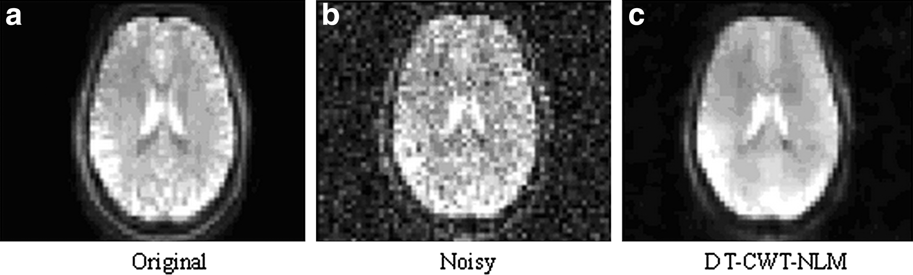
The results from simulation 1 (static data) consistently show that M=3 yields the highest PSNR (data not shown), which was then employed for simulation 2 (dynamic data) and the in vivo data. Figure 1 shows that DT-CWT-NLM largely removes noise, but well retains detailed information.

FIG. 1.

Simulation 1: (a) gold standard image. The image corresponds to the ASL calibration image (M0); (b) noisy image: 5% of Rician noise was added; (c) denoised image using DT-CWT combined with NLM. ASL, arterial spin labeling; DT-CWT, dual-tree complex wavelet transform; NLM, nonlocal means.

Figure 2 shows the results from simulation 2 regarding the sensitivity and accuracy in detecting functional networks from both noisy and denoised data with the following numbers of TPs: (a) TP=59 and (b) TP=100 (see Supplementary Fig. S1a, b; Supplementary Data are available online at www.liebertpub.com/brain for results from TP=200 and TP=300). Specifically, Table 1 shows that denoising leads to marked improvements in sensitivity with optimal thresholds (i.e., those corresponding to the highest accuracy). Not surprisingly, denoising achieves less gain in sensitivity with an increasing SNR or larger number of points and even led to a slightly lower sensitivity for one dataset (i.e., NL=25 and TP=200, Table 1 and Supplementary Fig. S1a, b); this is due to the fact that in those cases, the original (noisy) data are of sufficient quality to achieve good sensitivity. With respect to accuracy, Figure 2 demonstrates that consistently higher accuracy can be achieved by denoising the low SNR data tested, that is, SNR=3.7, regardless of the number of TPs (Table 1). Denoising achieves higher accuracy for data with 100 TPs (a value often used with ASL fMRI data), although the improvements are not as substantial (Note: this is due to the higher accuracy values for the original noisy data). As expected, denoising provides less benefit in improving accuracy with an increasing SNR. In particular, denoising unfavorably leads to slightly lower accuracy for data with a relatively high SNR, that is, low NL (SNR=5.0) and large number of TPs (200 and 300) (Supplementary Fig. S1a, b), likely due to the smoothing effect introduced by denoising.

FIG. 2.

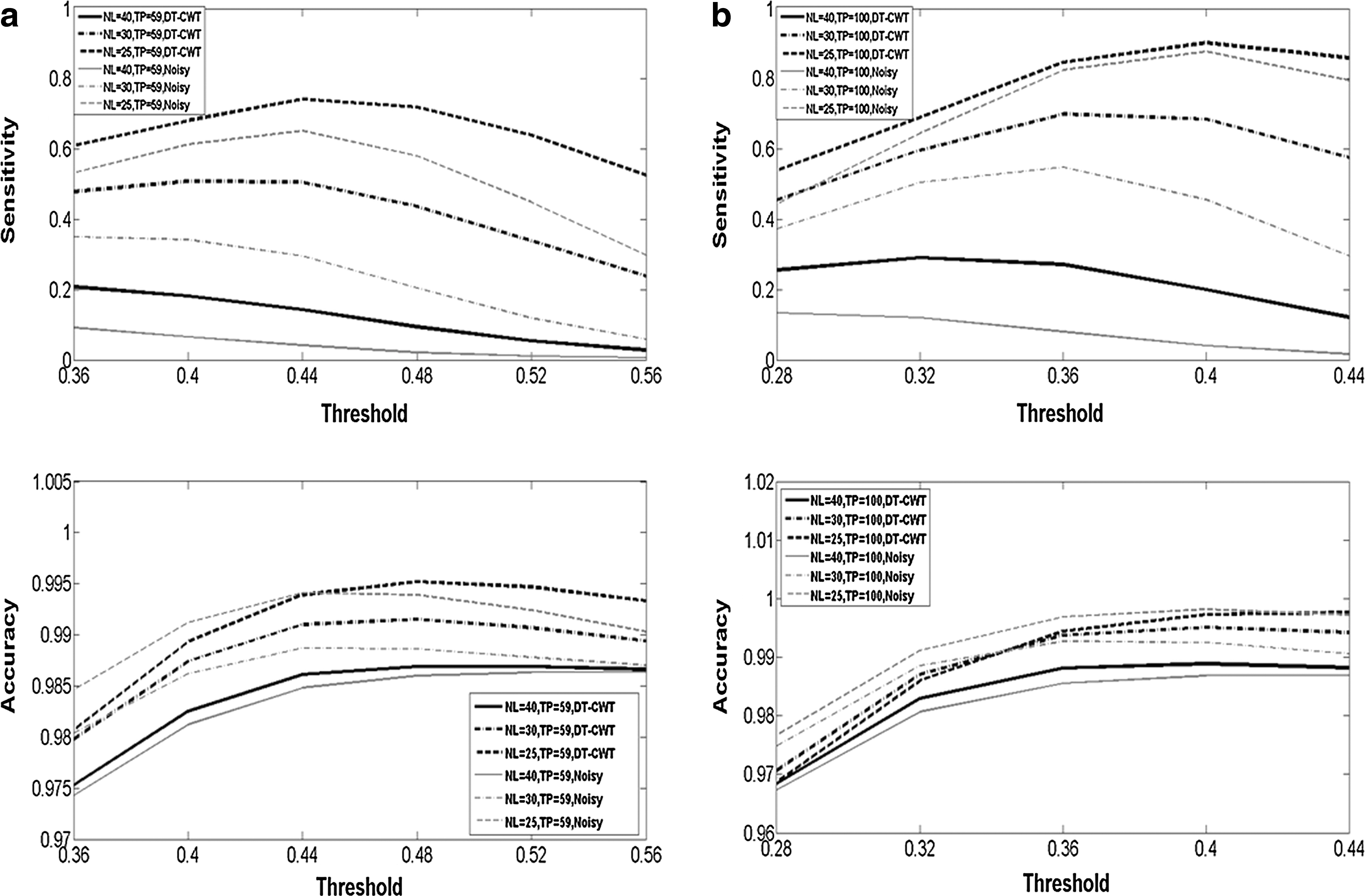
Simulation 2: plots of estimated values of sensitivity and accuracy in detecting simulated functional networks from both noisy data (gray thin lines) and denoised data using the DT-CWT-NLM (black thick lines) with two different numbers of TPs: (a) TP=59 and (b) TP=100, at three different levels of noise (SNR=5.0, 4.4, and 3.7). SNR, signal-to-noise ratio; TP, time point.

Table 1.

Sensitivity/Accuracy Percentage Changes Relative to Noisy Data by Denoising Using DT-CWT-NLM with Optimal Thresholds with Columns Representing Four Different TPs and Rows Representing Three Noise Levels

Noise level	TP=300	TP=200	TP=100	TP=59
25 (SNR=5.0)	0.3%/–0.32%	−0.3%/–0.03%	2.9%/0.04%	23.9%/0.13%
30 (SNR=4.4)	2.3%/–0.08%	8.6%/0.01%	50.0%/0.26%	71.4%/0.21%
40 (SNR=3.7)	360.0%/0.51%	304.0%/0.41%	400.0%/0.21%	248.7%/0.13%

DT-CWT, dual-tree complex wavelet transform; NLM, nonlocal means; SNR, signal-to-noise ratio; TP, time point.

Figure 3a demonstrates that DT-CWT-NLM has consistently better performance for data with the lowest SNR in our case (SNR=3.7) than without denoising in terms of the lower number of Fp+Fn regardless of TPs. However, for medium and high SNR, the superior performance of denoising is, in part, determined by the maximum number of TPs, that is, denoising results in improvement for TPs lower than ∼200 for data with a medium SNR (SNR=4.4, Fig. 3b) and for TPs lower than ∼100 for data with the highest SNR tested (SNR=5.0, Fig. 3c). While these findings are consistent with those in Figure 2, the plots of Fp+Fn more clearly demonstrate the superior performance of DT-CWT-NLM in denoising fMRI data with a relatively low SNR and small number of TPs. Given that any denoising inevitably leads to false positives, absolute number of false positives is therefore included (Fig. 4). In addition, for reference, ground truth of number of edges and null edges are as follows: ∼2 million and ∼144 million, respectively.

FIG. 3.

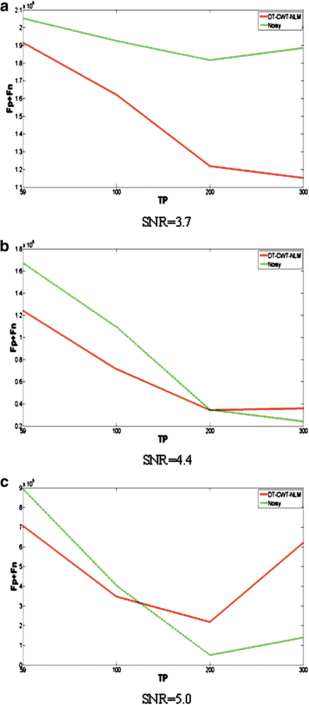
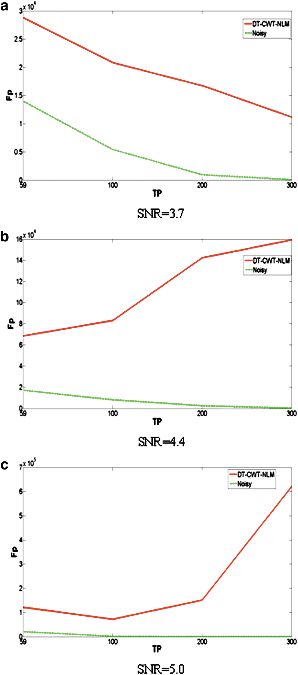
Simulation 2: plots of the sum of misclassification (Fp+Fn) in investigating functional connectivity from both noisy (dashed green lines) and denoised data using DT-CWT-NLM (solid red lines) with three different NLs: (a) SNR=3.7; (b) SNR=4.4; and (c) SNR=5.0. Fp and Fn represent false positives and false negatives, respectively. NL, noise level. Color images available online at www.liebertpub.com/brain

FIG. 4.

Simulation 2: plots of the total number of false positives (Fp) in investigating functional connectivity from both noisy (dashed green lines) and denoised data using DT-CWT-NLM (solid red lines) with three different NLs: (a) SNR=3.7; (b) SNR=4.4; and (c) SNR=5.0. Color images available online at www.liebertpub.com/brain

Figure 5 illustrates the extent to which denoising achieves noise reduction for the in vivo data from one typical subject, while still retaining the features of the original image. Visual inspection clearly shows that the proposed method greatly improves the ASL perfusion image quality.

FIG. 5.

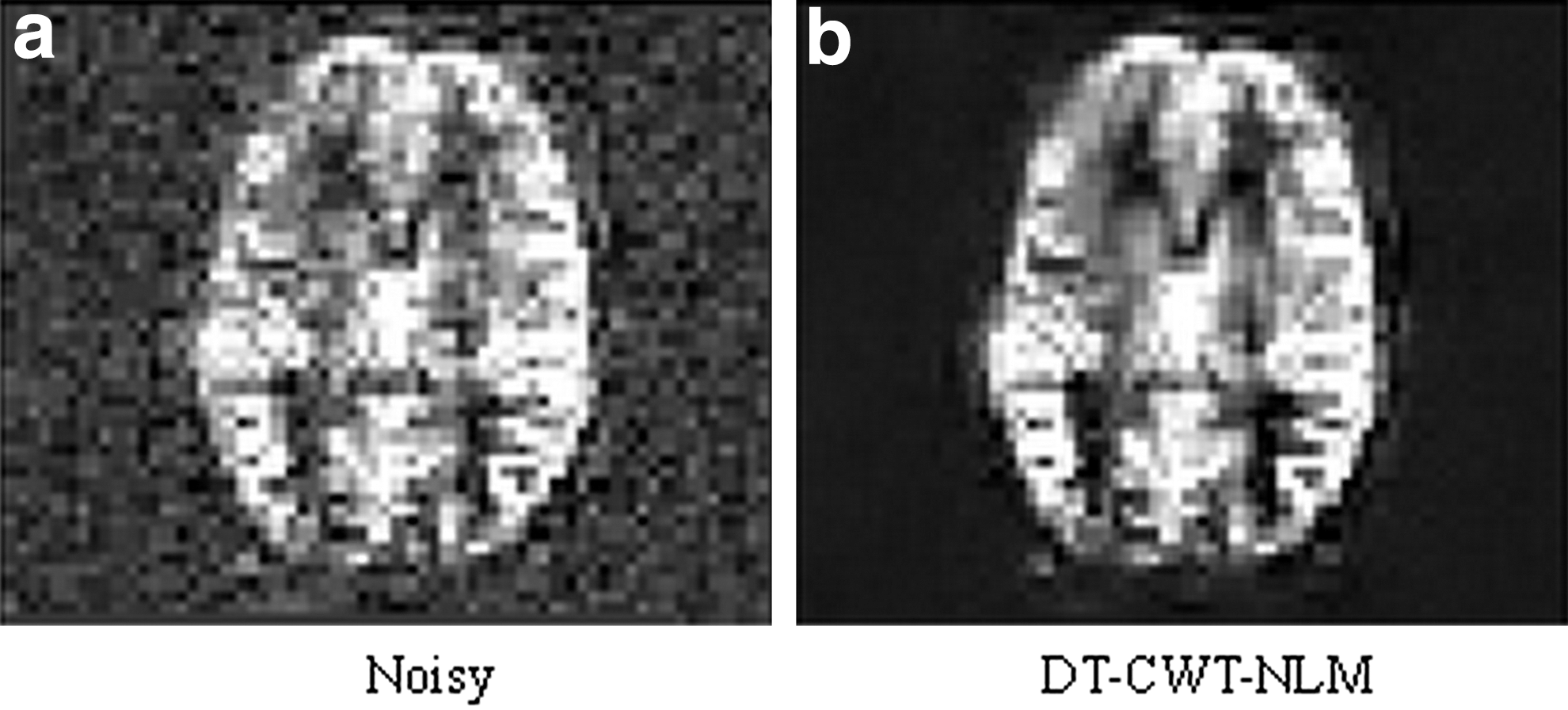
Illustration of the effect of denoising on the in vivo cerebral blood flow map generated from ASL for one typical subject: (a) before and (b) after denoising with the proposed method (DT-CWT combined with NLM).

Figure 6 shows histograms of voxel-wise degree distribution calculated from noisy and denoised in vivo data from three illustrative subjects. These results show a consistently higher histogram count toward the higher end of the degree range after denoising for each subject (Note that only the tail end of the histogram, i.e., with higher degrees, is displayed in this figure). For visualization purpose, voxels having degrees greater than a certain threshold (mean+standard deviation across whole brain) were considered as hub voxels. Figure 7 shows the hub maps for three illustrative subjects (the same subjects as in Fig. 6). It is clearly shown that more extensive and coherent hub voxels can be detected with denoising than without denoising.

FIG. 6.

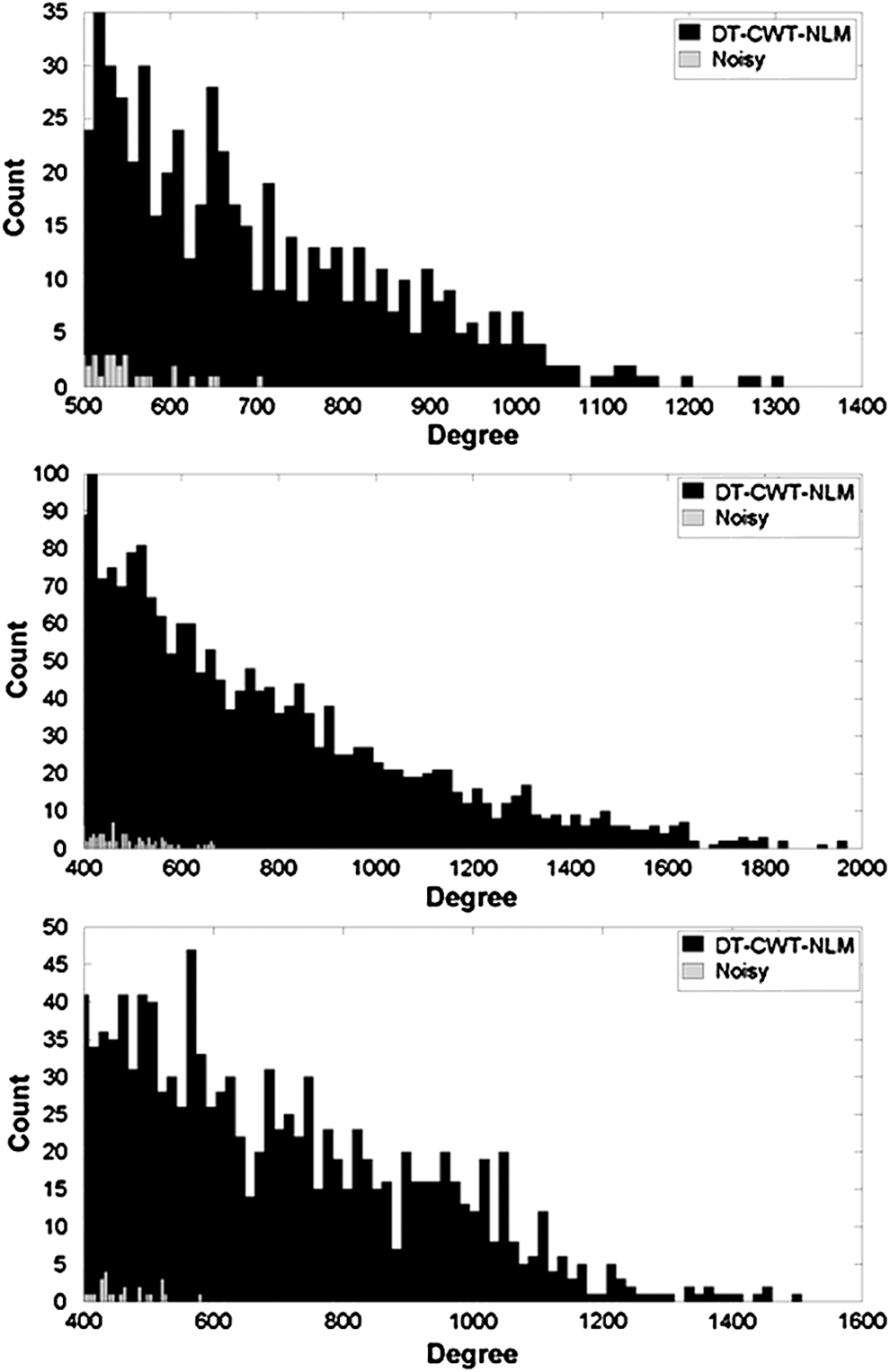
Histograms of voxel-wise degree distributions calculated from both noisy (gray) and denoised in vivo data using DT-CWT-NLM (black), x-axis: degrees, y-axis: count; results from three randomly chosen subjects are included. To aid visual assessment, the distributions were truncated to exclude the very small number of entries with very large degree numbers.

FIG. 7.

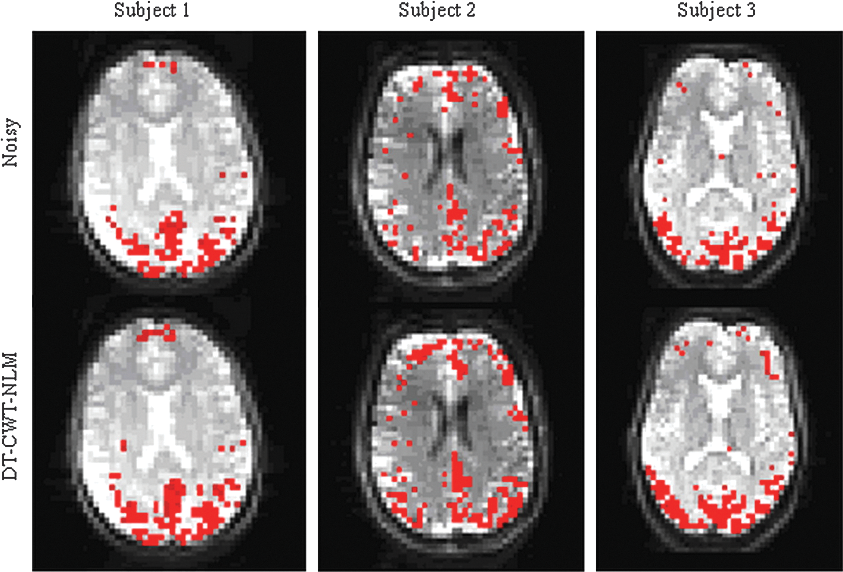
Hub voxels of the functional brain from three illustrative subjects (three columns, same subjects as in Fig. 6). The hub voxels detected without denoising (top) and with DT-CWT-NLM (bottom) are shown in axial views. Note: significantly more detected hub voxels are readily appreciated from denoised images using DT-CWT-NLM, most of which are located in the well-known default mode network. Color images available online at www.liebertpub.com/brain

Consistently higher values of efficiencies cost were found from denoised in vivo data than that from noisy data for all subjects studied (Fig. 8 and Supplementary Fig. S2). Taken together, these results further support the benefits of suitable denoising strategies for functional connectivity studies using ASL fMRI. Interestingly, the maximum efficiencies cost is achieved at approximately the same range of cost values [0.15, 0.2] for each subject, suggesting that the balance between efficiencies and cost can be attained consistently across subjects; this is in contrast to the large variability of thresholds from Pearson correlation. This could have a potential role in selection of an appropriate threshold (Discussion section).

FIG. 8.

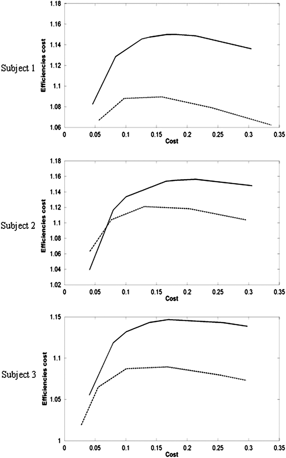
Values of efficiencies cost estimated from both denoised data and noisy data from three illustrative subjects (same as in Figs. 6 and 7). The values calculated from denoised data (solid lines) are consistently higher than those from noisy data (dotted lines). The maximum value of efficiencies cost is achieved at the cost range [0.15, 0.2] for each subject.

Figure 9 shows that the achievable maximum value of efficiencies cost calculated from one in vivo ASL data is increasingly lower with lower number of TPs (and therefore lower overall SNR). This suggests that denoising is expected to achieve higher values of efficiencies cost (i.e., higher SNR values are associated with higher efficiencies cost). As a proof of concept, Figure 9 therefore suggests that efficiencies cost was a meaningful quantitative measure to evaluate the performance of denoising in improving the SNR of in vivo ASL fMRI images, for example, as done in Figure 8. As was the case for the results shown in Figure 8, the maximum efficiencies cost can be achieved at the cost of about 0.15 for all cases.

FIG. 9.

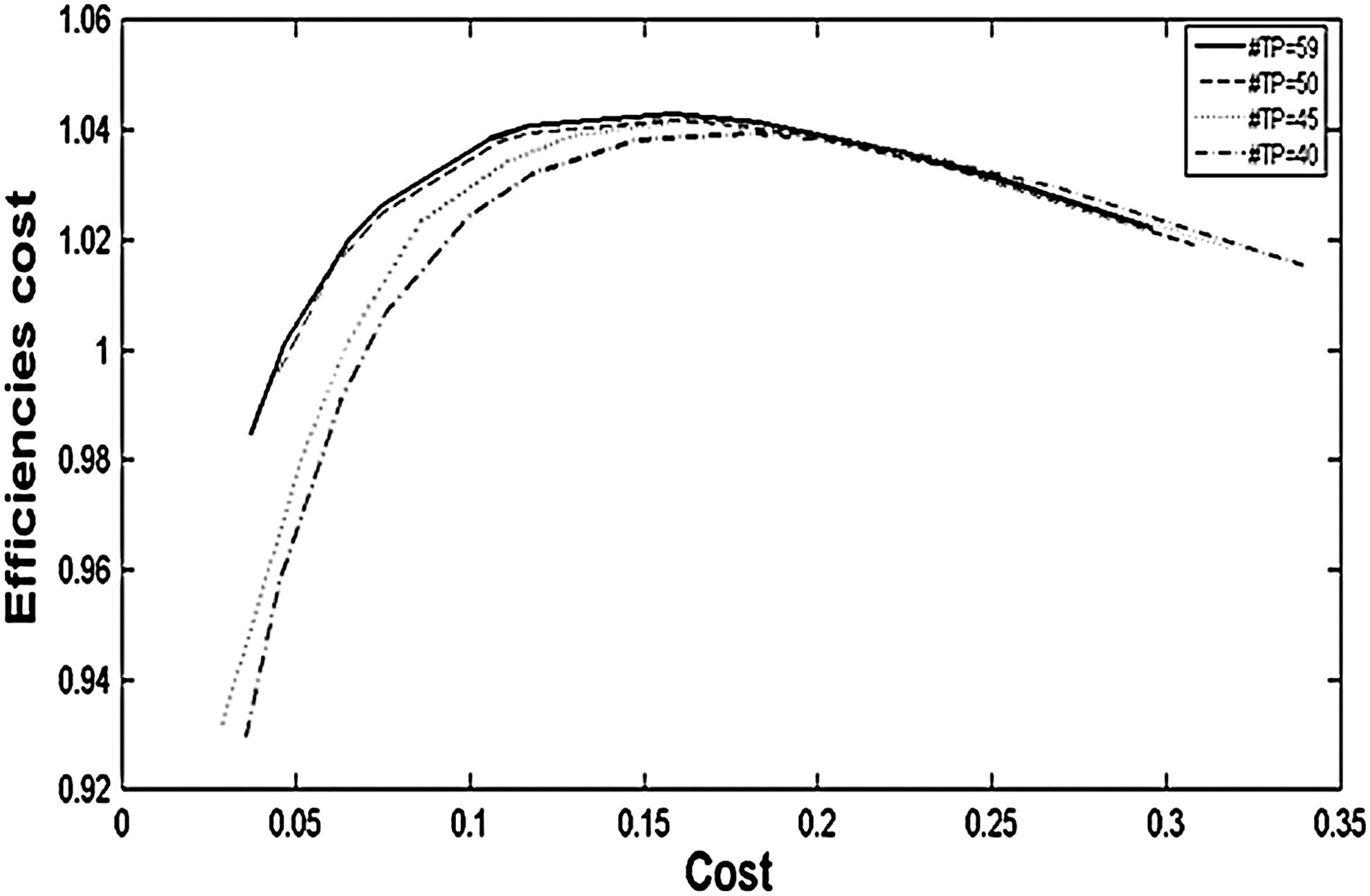
Comparisons of values of efficiencies cost corresponding to a range of cost calculated from one ASL dataset with four different TPs: 59, 50, 45, and 40, representing data with a decreasing SNR. The achievable maximum values of efficiencies cost (at around the cost of 0.15) calculated from data with a higher SNR are shown to be consistently higher than those from data with a lower SNR.

Our results show that mean and standard deviation of SNR calculated from all 10 subjects mostly overlap with the simulated data with two levels of noise (SNR=5.0 and 4.4, Supplementary Fig. S3). Therefore, the results from the simulations for these NLs are the ones that are of most relevance to our ASL in vivo protocol.

Discussion

In this study, voxel-wise functional connectomics was investigated using ASL fMRI, in particular addressing issues related to the intrinsically low SNR characteristics of ASL. To improve the SNR for voxel-wise functional connectivity studies, one could simply acquire more TPs. However, this might not be always feasible in practice due to limited scan time. Alternatively, an improved SNR could also be achieved by denoising.

In particular, a novel denoising method, DT-CWT combined with NLM, was proposed. This denoising method was shown to greatly improve the quality of the ASL data without oversmoothing the images. To evaluate the performance of the proposed denoising method in detecting voxel-wise functional networks, data were simulated to include different levels of noise and different number of TPs; those noise-free data were employed as gold standards to calculate the accuracy and sensitivity of detecting functional networks. The methodology was also evaluated using in vivo ASL fMRI data; in this case, due to the lack of gold standards, the measure of efficiencies cost was proposed as a quantitative means to assess the performance in detecting functional networks. Quantitative analysis of both simulations and in vivo data showed that denoising greatly benefits detection of voxel-wise functional networks from data with a low SNR and small number of TPs, such as it is often the case with ASL fMRI.

The validity of the proposed denoising method has been confirmed with dynamic data by simulation 2, in which higher accuracy and sensitivity of voxel-wise functional connectomics was achieved from low SNR data with DT-CWT-NLM denoising than that without denoising. However, as expected from any denoising method, very limited benefit was observed for the case of high-quality data, that is, data with a high SNR and/or a large number of TPs. In fact, no denoising is required for high-quality data, given that the inherent smoothing effect associated with any denoising algorithms will outweigh the gain achieved by a further increase in SNR. Nonetheless, it should be noted that relatively low sensitivity (∼0.5) was achieved when data have relatively low SNR (NL=30 and SNR=4.4) and small number of TPs (59), a situation not altogether uncommon with in vivo ASL data. By increasing TPs, sensitivity can be largely increased (∼0.7, ∼0.9, and ∼0.9 for TP=100, 200, and 300, respectively), which suggests that if practically feasible, more TP measurements should be acquired to ensure both high accuracy and sensitivity for in vivo ASL data. Nonetheless, as shown in simulation 2, our denoising method did improve the accuracy and sensitivity in detecting functional networks from those data with a low SNR or small number of TPs.

The histograms from degree connections from the in vivo data were much broader for denoised data than those without denoising, indicating that an increased number of connections can be detected with denoising. While it is likely that some false positives may be also introduced, the results from simulation 2 suggest that the overall higher accuracy and sensitivity for low SNR data corroborate the validity of denoising in improving detection of voxel-wise functional networks from in vivo ASL fMRI data.

The newly proposed evaluation criterion, efficiencies cost, was chosen to account for the fact that although efficiencies (global/local) are often employed to characterize networks and can then be compared across groups, efficiencies themselves might not be suitable for evaluating the optimality of the network estimated from denoised data against that from noisy data. This is because, for small-world networks, a denser network always has higher global and local efficiencies than a sparser network. Given the biological definitions of global and local efficiencies and cost (Achard and Bullmore, 2007), the efficiencies cost provides a biologically meaningful criterion to evaluate the performance of denoising in detecting functional networks. Consistently higher values of efficiencies cost across subjects suggest that a more optimal network is generated from denoised data than data without denoising. This was corroborated by the results that higher efficiencies cost can be achieved by increasing number of TPs (59 vs. 50, 45, and 40, respectively). Essentially, denoising has the same goal of increasing SNR as the method of increasing TPs.

For simulation 2, we used a range of thresholds to estimate the highest accuracy and sensitivity achieved in detecting voxel-wise functional networks; however, the choice of threshold remains an open question. Based on in vivo calculated values of efficiencies cost in all the 10 subjects, we observed that the maximum values were consistently achieved for thresholds that lead to a cost in the range∼[0.15, 0.2]. It is likely that the threshold corresponding to the cost achieving a maximum efficiencies cost corresponds to the optimal threshold. This possible criterion to select an appropriate threshold appears promising and valuable; however, further studies are warranted to evaluate its feasibility.

Methodological issues and future work

Denoising methods could introduce spatial smoothing. To minimize this effect, the proposed method uses NLM that avoids local averaging (Buades et al., 2005a). However, any smoothing (even the small residual smoothing) inevitably leads to some false correlations, and false correlations might lead to false edges (false positives and false negatives), which reduce accuracy and sensitivity, as well as distorting node degree distribution. Specifically, for our in vivo ASL protocol (SNR=4.4 and TP=59), Figure 4 shows that denoising unfavorably causes more false positives than noisy data; however, Figure 3 indicates that denoising can in turn lead to a decrease in false negatives that is one order of magnitude greater than increase in false positives caused by denoising. The presence of false edges would inevitably affect efficiency cost as well. However, it should be noted that denoising should also favorably increase the true positive rate, which combined with the reduced false negative rate is predominantly advantageous over the moderate false correlations caused by denoising, as evidenced by the results of our simulations and in vivo results. Overall, optimum denoising approaches should contribute to improving accuracy and sensitivity in detecting functional networks.

Another factor that needs to be considered is partial volume effect, which is a well-known source of error in ASL studies due to their low spatial resolution. Partial volume effect is more problematic for voxel-wise functional connectivity studies than for region-based studies. However, this issue could be addressed to a certain extent by employing methods for correcting the partial volume effect (Asllani et al., 2008; Liang et al., 2013).

In our particular implementation of the ASL sequence, a k-space sharing strategy was used (Liang et al., 2012a); this inevitably leads to a certain degree of temporal smoothing, primarily on the high-frequency image detail. Thus, low-frequency physiological noise and BOLD components might contaminate the ASL signal. Nonetheless, this effect is likely to be minor, as supported by the previously shown capability of this acquisition strategy in investigating functional connectivity (Liang et al., 2012a, 2014a). It should be noted, however, that the use of the k-space sharing strategy is not central to the findings from the current study and, in particular, the benefits of denoising ASL data for voxel-wise functional connectomics should be independent of the specific acquisition strategy used.

Last, simulated data in simulation 2 did not consider the ASL sequence used and only random noise was considered; this might not accurately model the real ASL fMRI data, which can also contain physiological noise and motion artifacts. The estimated accuracy and sensitivity in detecting functional networks are therefore likely to deviate to some extent from the values in reality.

Conclusion

In this study, voxel-wise functional connectivity was investigated using ASL fMRI. Given that the ASL signal has an intrinsically low SNR, as an intermediate aim, a novel denoising method, DT-CWT combined with NLM, was proposed to improve the intrinsically low SNR of ASL signal. Both simulations and in vivo ASL data showed that denoising is effective in improving the detection of voxel-wise functional networks from noisy data. Given the potential advantages of ASL over BOLD fMRI (Liu and Brown, 2007), this study demonstrates that ASL fMRI in conjunction with appropriate denoising should provide a useful complementary technique in investigating the brain connectome.

Footnotes

Author Disclosure Statement

No competing financial interests exist.

References

Achard

, Bullmore

. 2007. Efficiency and cost of economical brain functional networks. PLoS Comput Biol, 3:e17.

Achard

, Salvador

, Whitcher

, Suckling

, Bullmore

. 2006. A resilient, low-frequency, small-world human brain functional network with highly connected association cortical hubs. J Neurosci, 26:63–72.

Aslan

, Xu

, Wang

, Uh

, Yezhuvath

, Van Osch

, Lu

. 2010. Estimation of labeling efficiency in pseudocontinuous arterial spin labeling. Magn Reson Med, 63:765–771.

Asllani

, Borogovac

, Brown

. 2008. Regression algorithm correcting for partial volume effects in arterial spin labeling MRI. Magn Reson Med, 60:1362–1371.

Balster

, Zheng

, Ewing

. 2005. Feature-based wavelet shrinkage algorithm for image denoising. IEEE Trans Image Process, 14:2024–2039.

Bibic

, Knutsson

, Stahlberg

, Wirestam

. 2010. Denoising of arterial spin labeling data: wavelet-domain filtering compared with Gaussian smoothing. MAGMA, 23:125–137.

Boxerman

, Bandettini

, Kwong

, Baker

, Davis

, Rosen

, Weisskoff

. 1995. The intravascular contribution to fMRI signal change: Monte Carlo modeling and diffusion-weighted studies in vivo. Magn Reson Med, 34:4–10.

Buades

, Coll

, Morel

. 2005a. A non-local algorithm for image denoising. 2005 IEEE Computer Society Conference on Computer Vision and Pattern Recognition, Vol 2, Proceedings, 60–65.

Buades

, Coll

, Morel

. 2005b. A review of image denoising algorithms, with a new one. Multiscale Model Simul, 4:490–530.

10.

Bullmore

, Sporns

. 2009. Complex brain networks: graph theoretical analysis of structural and functional systems. Nat Rev Neurosci, 10:186–198.

11.

Bullmore

, Sporns

. 2012. The economy of brain network organization. Nat Rev Neurosci, 13:336–349.

12.

Buxton

, Uludag

, Dubowitz

, Liu

. 2004. Modeling the hemodynamic response to brain activation. Neuroimage, 23:S220–S233.

13.

Chuang

, van Gelderen

, Merkle

, Bodurka

, Ikonomidou

, Koretsky

, Duyn

, Talagala

. 2008. Mapping resting-state functional connectivity using perfusion MRI. Neuroimage, 40:1595–1605.

14.

Coupe

, Hellier

, Prima

, Kervrann

, Barillot

. 2008a. 3D wavelet subbands mixing for image denoising. Int J Biomed Imaging, 2008:590183.

15.

Coupe

, Manjon

, Gedamu

, Arnold

, Robles

, Collins

. 2009. An object-based method for Rician noise estimation in MR images. Med Image Comput Comput Assist Interv, 12:601–608.

16.

Coupe

, Yger

, Prima

, Hellier

, Kervrann

, Barillot

. 2008b. An optimized blockwise nonlocal means denoising filter for 3-D magnetic resonance images. IEEE Trans Med Imaging, 27:425–441.

17.

Garcia

, Duhamel

, Alsop

. 2005. Efficiency of inversion pulses for background suppressed arterial spin labeling. Magn Reson Med, 54:366–372.

18.

Gonzalez-At

, Alsop

, Detre

. 2000. Cerebral perfusion and arterial transit time changes during task activation determined with continuous arterial spin labeling. Magn Reson Med, 43:739–746.

19.

Hayasaka

, Laurienti

. 2010. Comparison of characteristics between region-and voxel-based network analyses in resting-state fMRI data. Neuroimage, 50:499–508.

20.

Liang

, Connelly

, Calamante

. 2013. Improved partial volume correction for single inversion time arterial spin labeling data. Magn Reson Med, 69:531–537.

21.

Liang

, Connelly

, Calamante

. 2014a. Graph analysis of resting-state ASL perfusion MRI data: nonlinear correlations among CBF and network metrics. Neuroimage, 87:265–275.

22.

Liang

, Connelly

, Calamante

. 2014b. A novel method for robust estimation of group fucntional connectivity based on a joint graphical models approach. In: Proceedings of ISMRM 21th Annual Meeting, Milan, Italy, p3059.

23.

Liang

, Tournier

, Masterton

, Connelly

, Calamante

. 2012a. A k-space sharing 3D GRASE pseudocontinuous ASL method for whole-brain resting-state functional connectivity. Int J Imaging Syst Technol, 22:37–43.

24.

Liang

, Wang

, Yan

, Shu

, Xu

, Gong

, He

. 2012b. Effects of different correlation metrics and preprocessing factors on small-world brain functional networks: a resting-state functional MRI study. PLoS One, 7:e32766.

25.

Liu

, Brown

. 2007. Measurement of cerebral perfusion with arterial spin labeling: part 1. Methods. J Int Neuropsychol Soc, 13:517–525.

26.

Malfait

, Roose

. 1997. Wavelet-based image denoising using a Markov random field a priori model. IEEE Trans Image Process, 6:549–565.

27.

Peng

, Wang

, Zhou

, Zhu

. 2009. Partial correlation estimation by joint sparse regression models. J Am Stat Assoc, 104:735–746.

28.

Rubinov

, Sporns

. 2010. Complex network measures of brain connectivity: uses and interpretations. Neuroimage, 52:1059–1069.

29.

Salvador

, Suckling

, Coleman

, Pickard

, Menon

, Bullmore

. 2005. Neurophysiological architecture of functional magnetic resonance images of human brain. Cereb Cortex, 15:1332–1342.

30.

Selesnick

, Baraniuk

, Kingsbury

. 2005. The dual-tree complex wavelet transform. IEEE Signal Process Mag, 22:123–151.

31.

Smith

. 2012. The future of FMRI connectivity. Neuroimage, 62:1257–1266.

32.

Stam

, Reijneveld

. 2007. Graph theoretical analysis of complex networks in the brain. Nonlinear Biomed Phys, 1:3.

33.

Tzourio-Mazoyer

, Landeau

, Papathanassiou

, Crivello

, Etard

, Delcroix

, Mazoyer

, Joliot

. 2002. Automated anatomical labeling of activations in SPM using a macroscopic anatomical parcellation of the MNI MRI single-subject brain. Neuroimage, 15:273–289.

34.

Utevsky

, Smith

, Huettel

. 2014. Precuneus is a functional core of the default-mode network. J Neurosci, 34:932–940.

35.

van Den Heuvel

, Stam

, Boersma

, Hulshoff Pol

. 2008. Small-world and scale-free organization of voxel-based resting-state functional connectivity in the human brain. Neuroimage, 43:528–539.

36.

Watts

, Strogatz

. 1998. Collective dynamics of ‘small-world’ networks. Nature, 393:440–442.

37.

Wells

, Thomas

, King

, Connelly

, Lythgoe

, Calamante

. 2010. Reduction of errors in ASL cerebral perfusion and arterial transit time maps using image de-noising. Magn Reson Med, 64:715–724.

38.

Wink

, Roerdink

. 2004. Denoising functional MR images: a comparison of wavelet denoising and Gaussian smoothing. IEEE Trans Med Imaging, 23:374–387.

Supplementary Material

Please find the following supplemental material available below.

For Open Access articles published under a Creative Commons License, all supplemental material carries the same license as the article it is associated with.

For non-Open Access articles published, all supplemental material carries a non-exclusive license, and permission requests for re-use of supplemental material or any part of supplemental material shall be sent directly to the copyright owner as specified in the copyright notice associated with the article.

0.00 MB

0.23 MB

0.10 MB

0.03 MB