The Impact of Normalization and Segmentation on Resting-State Brain Networks

Abstract

Graph theory has recently received a lot of attention from the neuroscience community as a method to represent and characterize brain networks. Still, there is a lack of a gold standard for the methods that should be employed for the preprocessing of the data and the construction of the networks, as well as a lack of knowledge on how different methodologies can affect the metrics reported. The authors used graph theory analysis applied to resting-state functional magnetic resonance imaging to investigate the influence of different node-defining strategies and the effect of normalizing the functional acquisition on several commonly reported metrics used to characterize brain networks. The nodes of the network were defined using either the individual FreeSurfer segmentation of each subject or the FreeSurfer segmented Montreal National Institute (MNI) 152 template, using the Destrieux and subcortical atlas. The functional acquisition was either kept on the functional native space or normalized into MNI standard space. The comparisons were done at three levels: on the connections, on the edge properties, and on the network properties levels. The results reveal that different registration and brain parcellation strategies have a strong impact on all the levels of analysis, possibly favoring the use of individual segmentation strategies and conservative registration approaches. In conclusion, several technical aspects must be considered so that graph theoretical analysis of connectivity MRI data can provide a framework to understand brain pathologies.

Introduction

The brain remains, to this day, as one of the most enigmatic organs in the human body. The inherent difficulty to understand its wiring patterns and how they relate to different functions brought the necessity to explore new methods that can bring new light on this subject (Stam and Reijneveld, 2007). One such method that has received increasing attention in the last decade is graph theory and the study of complex networks. One of the core strengths of graph theory in brain network modeling lies in its ability to quantitatively characterize the topological organization of the brain (He and Evans, 2010). It can have a key role in the interpretation of the complex dynamics detected in the brain across different studies using different modalities and models. Starting in the 90s [see for a review Ref. (Sporns, 2012)], several key moments revolutionized the study of brain connectivity, namely the introduction of the functional magnetic resonance imaging (fMRI) technique (Ogawa et al., 1990), the first studies that demonstrated the potential of the analysis of brain connectivity patterns (Felleman and Van Essen, 1991; Sporns et al., 1991; Young, 1992), the association of memory mechanisms to different mental states and connectivity patterns (McIntosh et al., 1997, 1999), and the introduction of the concept of small-world networks (Watts and Strogatz, 1998). More recently, multiple studies have shown the potential of the application of graph theory to represent and characterize brain networks. While there are reports of the application of graph theory with different imaging techniques, such as electroencephalography, magnetoencephalography (Yu et al., 2008), and positron emission tomography (Huang et al., 2010), MRI is by far the most common (Bullmore and Sporns, 2009; Lang et al., 2012).

A graph is a mathematical abstraction that can be understood as a group of nodes, which represent the different elements of the network, linked by edges, representing some relationship between them (Gross and Yellen, 2006). Translating these components into a brain network is fairly simple in concept; each node can represent an anatomic unit of the brain (can theoretically range from individual cells to full anatomic structures) and the edges can represent different relationships between regions, like the statistical correlation of fMRI activations, the number/density of connecting fibers obtained through diffusion tractography, or structural properties such as cortical thickness correlations. Despite the many advantages of using graph theory as a model for brain connectivity, some key issues still ensue. Building a brain graph means making a lot of decisions and assumptions that can directly affect the outcome and the results arising from different processing strategies cannot be easily compared (Bullmore and Bassett, 2011). It has been demonstrated that different properties of the network behave differently with connection type (Liang et al., 2012), network size, edge density, and degree distribution (van Wijk et al., 2010), especially the small-world parameters, depending on the number of nodes and the average degree of the network (Wang et al., 2009).

Different node-defining strategies can vary greatly on the number of nodes used, ranging from very small networks with 19 nodes (Lord et al., 2011) to the most common number of 90 nodes from the Automated Anatomic Labeling atlas (Hosseini and Kesler, 2013; Richiardi et al., 2011; Tian et al., 2011), and building up to much bigger networks ranging from 998 nodes (Hagmann et al., 2007) and up to 10,000 (van den Heuvel et al., 2008). The choice of the nodes definition can also vary from the use of a presegmented atlas in a standard space (Achard et al., 2006; Sun et al., 2012), the use of segmentation tools to individually parcellate each subject's brain (Minati et al., 2012; Richiardi et al., 2011), brain activation clusters extracted from fMRI analysis (Sun et al., 2012; Vandenberghe et al., 2013), or simply to the use of all voxels in the image (van den Heuvel et al., 2008). Such diversity of possibilities demands a thorough knowledge on how these might affect the characteristics of the network in all its range of possibilities.

Another key difference between studies is the choice of fundamental preprocessing steps: some studies normalize the images to a standard space (Achard et al., 2006; Lord et al., 2011; Minati et al., 2012; Tian et al., 2011), while others do not (Sun et al., 2012; van den Heuvel et al., 2008); some apply spatial smoothing steps with differently sized kernels (Lord et al., 2011; Minati et al., 2012; Sun et al., 2012), while others do not (Achard et al., 2006; Tian et al., 2011); some apply signal regression to remove confound signals (Achard et al., 2006; Lord et al., 2011; Minati et al., 2012), while others do not (Richiardi et al., 2011; Tian et al., 2011; van den Heuvel et al., 2008); and finally, different frequency filtering strategies can also be found (Achard and Bullmore, 2007; Liang et al., 2012; Supekar et al., 2009).

There is an obvious need to have the functional images (originally on its native space) and the node-defining images (usually on a standard space) in a common space. While the most common approach to achieve this is to normalize the functional images to the standard space, the opposite is still a valid, rather unused, option. Although, as hypothesized in another study (van den Heuvel et al., 2008), the interpolation of the voxels that occurs during this step can introduce artificial correlations, the effect of the normalization step on the networks is still largely unexplored.

On the brain parcellation strategies, the most common approach is to simply coregister the functional images and a fixed template, resuming the segmentation to the normalization step. A more elaborate alternative is to employ tools to individually segment each subject, such as FreeSurfer (Fischl, 2012). This strategy takes more factors into consideration (such as surface matching and gyri and sulci identification) and is known to produce more accurate results (Destrieux et al., 2010). The impact of these different procedures on the resulting networks is still unknown.

All these different possibilities may be responsible for some of the differences found, in the metrics that characterize the networks, between different studies having a direct impact on the conclusions that can be drawn from its results. In this work, the authors will focus on the study of two critical issues: the effect of normalizing the fMRI images and the effect that different node-defining strategies (i.e., the use of individual parcellation methods versus the simple superposition of a fixed template) have on the resulting networks.

Materials and Methods

Ethics statement

The study was conducted in accordance with the principles expressed in the Declaration of Helsinki and was approved by the Ethics Committee of Hospital de Braga (Portugal).

Subjects and acquisitions

In the current study, the MRI acquisitions of 59 healthy volunteers were used, from which 4 were discarded due to excess of movement during the acquisition, so that all subjects displayed head motion less than 2 mm in translation or 1 degree in rotation. Thus, a total of 55 subjects from the SWITCHBOX project were used in this study (31 males and 24 females aged between 51 and 82 years old and with a mean age of 64.85±8.82 years). The goals and tests of the study were explained to all participants, who provided informed written signed consent.

Two different acquisitions from each subject were used: as structural acquisition, a T1 magnetization-prepared rapid gradient echo with repetition time (TR)=2730 msec, echo time (TE)=3.5 msec, field of view (FoV)=256×256 mm, flip angle=7°, in-plane resolution of 1×1 mm, and 1 mm slice thickness; as a resting-state functional acquisition, a T2* echo-planar imaging acquisition with 180 volumes, TR=2000 msec, TE=30 msec, FoV=224×224 mm, flip angle=90°, in-plane resolution of 3.5×3.5 mm, and 4.5 mm slice thickness. All acquisitions were performed on a clinically approved Siemens Magnetom Avanto 1.5 T (Siemens Medical Solutions, Elangen, Germany) scanner, in Hospital de Braga, using a 12-channel receive-only Siemens head coil. During the resting-state acquisition, all subjects were instructed to remain with their eyes closed and to not think of anything in particular.

Preprocessing strategies

All fMRI images were preprocessed using BrainCAT (Marques et al., 2013), and the Matlab (v.2009b, www.mathworks.com) toolbox Conn (Whitfield-Gabrieli and Nieto-Castanon, 2012). fMRI preprocessing steps included the removal of the first 5 volumes, motion correction, slice-timing correction, skull stripping, band-pass temporal filtering (0.01–0.08 Hz) using BrainCAT, and the removal of the white matter (WM) and cerebrospinal fluid confound signals using Conn and the CompCor strategy (Behzadi et al., 2007).

While the usual procedure in functional studies is to normalize all images to a standard space (e.g., Montreal National Institute [MNI]) (Mazziotta et al., 2001), this step will, no matter how good the interpolation function is, alter the original data. To evaluate the effects of the normalization, two different strategies were tested: the normalization of all images to MNI standard space with 2 mm isotropic voxel size and the registration of all the support data (both the T1 structural data and the masks defining the nodes) to the native space of the functional acquisition of each subject. These strategies will allow testing if the normalization procedures can directly affect the network properties. Normalization and registration of all images was done using FSL FLIRT (Jenkinson and Smith, 2001) for each subject from the native functional image to the T1 anatomical image, using a rigid body transformation (6 degrees of freedom [dof]), and from the T1 image native space to the MNI standard space, using an affine transformation (12 dof). The concatenation and inversion of both transformation matrices allows for the registration from the functional native space to the MNI standard space and vice versa.

Graph construction

The construction of the graph encompasses two different stages, the definition of the nodes and the definition of the edges. On the node definition, two different strategies were compared, the use of a fixed template atlas, which was overlaid into each subject's acquisition, and the use of individually segmented images for each subject performed by applying the FreeSurfer v5.1 semiautomated workflow (Fischl, 2012). To eliminate the effect of comparing networks with different sizes (van Wijk et al., 2010) and different regions (Wang et al., 2009) derived from the use of different atlases, the MNI 152 brain template was segmented using the same FreeSurfer workflow, and thus creating the fixed template atlas. For both strategies, regions from two different segmentations were combined, 146 regions from the Destrieux cortical atlas (Destrieux et al., 2010) and 14 regions from the subcortical segmentation (Fischl et al., 2002), resulting in a total of 160 regions (Table 1 and Fig. 1). These two different node-defining strategies allowed us to test the effect of building networks with different parcellation strategies.

FIG. 1.

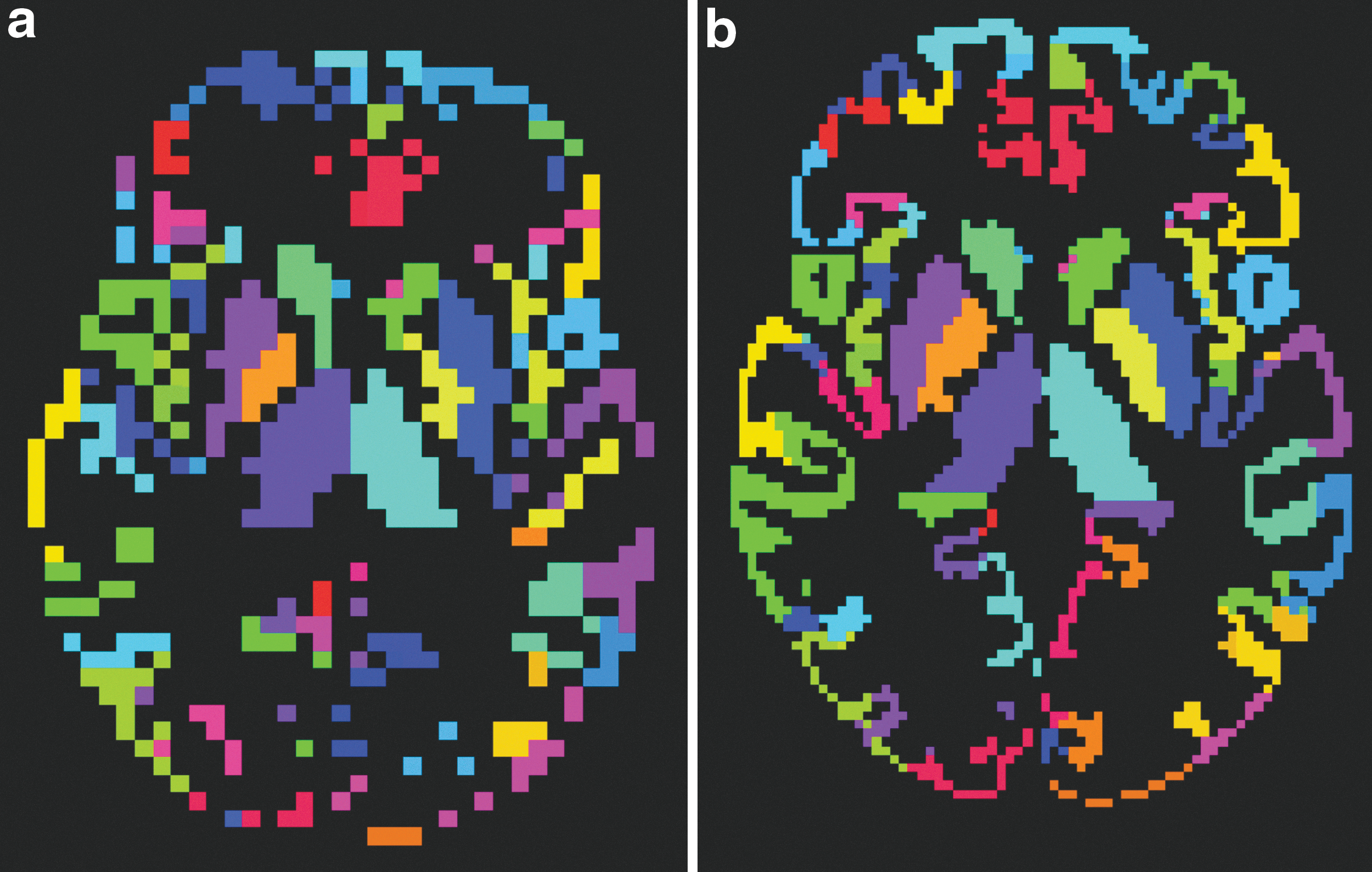
Axial view of the ROIs defined for one subject after preprocessing: (a) in native functional space; (b) in MNI space. MNI, Montreal National Institute; ROIs, regions of interest.

Table 1.

Regions of Interest Used from the Destrieux and Subcortical Atlas

Designation
lh/rh-Thalamus-Proper	ctx_lh/rh_G_temp_sup-Lateral
lh/rh-Caudate	ctx_lh/rh_G_temp_sup-Plan_polar
lh/rh-Putamen	ctx_lh/rh_G_temp_sup-Plan_tempo
lh/rh-Pallidum	ctx_lh/rh_G_temporal_inf
lh/rh-Hippocampus	ctx_lh/rh_G_temporal_middle
lh/rh-Amygdala	ctx_lh/rh_Lat_Fis-ant-Horizont
lh/rh-Accumbens-area	ctx_lh/rh_Lat_Fis-ant-Vertical
ctx_lh/rh_G_and_S_frontomargin	ctx_lh/rh_Lat_Fis-post
ctx_lh/rh_G_and_S_occipital_inf	ctx_lh/rh_Pole_occipital
ctx_lh/rh_G_and_S_paracentral	ctx_lh/rh_Pole_temporal
ctx_lh/rh_G_and_S_subcentral	ctx_lh/rh_S_calcarine
ctx_lh/rh_G_and_S_transv_frontopol	ctx_lh/rh_S_central
ctx_lh/rh_G_and_S_cingul-Ant	ctx_lh/rh_S_cingul-Marginalis
ctx_lh/rh_G_and_S_cingul-Mid-Ant	ctx_lh/rh_S_circular_insula_ant
ctx_lh/rh_G_and_S_cingul-Mid-Post	ctx_lh/rh_S_circular_insula_inf
ctx_lh/rh_G_cingul-Post-dorsal	ctx_lh/rh_S_circular_insula_sup
ctx_lh/rh_G_cingul-Post-ventral	ctx_lh/rh_S_collat_transv_ant
ctx_lh/rh_G_cuneus	ctx_lh/rh_S_collat_transv_post
ctx_lh/rh_G_front_inf-Opercular	ctx_lh/rh_S_front_inf
ctx_lh/rh_G_front_inf-Orbital	ctx_lh/rh_S_front_middle
ctx_lh/rh_G_front_inf-Triangul	ctx_lh/rh_S_front_sup
ctx_lh/rh_G_front_middle	ctx_lh/rh_S_interm_prim-Jensen
ctx_lh/rh_G_front_sup	ctx_lh/rh_S_intrapariet_and_P_trans
ctx_lh/rh_G_Ins_lg_and_S_cent_ins	ctx_lh/rh_S_oc_middle_and_Lunatus
ctx_lh/rh_G_insular_short	ctx_lh/rh_S_oc_sup_and_transversal
ctx_lh/rh_G_occipital_middle	ctx_lh/rh_S_occipital_ant
ctx_lh/rh_G_occipital_sup	ctx_lh/rh_S_oc-temp_lat
ctx_lh/rh_G_oc-temp_lat-fusifor	ctx_lh/rh_S_oc-temp_med_and_Lingual
ctx_lh/rh_G_oc-temp_med-Lingual	ctx_lh/rh_S_orbital_lateral
ctx_lh/rh_G_oc-temp_med-Parahip	ctx_lh/rh_S_orbital_med-olfact
ctx_lh/rh_G_orbital	ctx_lh/rh_S_orbital-H_Shaped
ctx_lh/rh_G_pariet_inf-Angular	ctx_lh/rh_S_parieto_occipital
ctx_lh/rh_G_pariet_inf-Supramar	ctx_lh/rh_S_postcentral
ctx_lh/rh_G_parietal_sup	ctx_lh/rh_S_precentral-inf-part
ctx_lh/rh_G_postcentral	ctx_lh/rh_S_precentral-sup-part
ctx_lh/rh_G_precentral	ctx_lh/rh_S_suborbital
ctx_lh/rh_G_precuneus	ctx_lh/rh_S_subparietal
ctx_lh/rh_G_rectus	ctx_lh/rh_S_temporal_inf
ctx_lh/rh_G_subcallosal	ctx_lh/rh_S_temporal_sup
ctx_lh/rh_G_temp_sup-G_T_transv	ctx_lh/rh_S_temporal_transverse

Using these masks, the mean signal across the voxels of each region was extracted from each time point of the fMRI acquisition, allowing for the final extraction of the time series. To measure the similarity between the time series, establishing a measure of functional connectivity (edges) between the corresponding regions of interest (ROIs), the Pearson correlation coefficient was used. The Pearson coefficient of each possible combination of ROIs was calculated in Conn and used to build a correlation matrix for each subject. The Fisher's r-to-Z transformation was then used to transform the r-values of the correlations into Z-values.

Combining the two different preprocessing and node-defining strategies, four different networks were computed for each subject, with the functional images in the MNI standard space (MNI networks) using the fixed template atlas (ATL-MNI) and the individual FreeSurfer segmentation (FS-MNI), and the functional native space (NAT networks) using the fixed template atlas (ATL-NAT) and the individual FreeSurfer segmentation (FS-NAT).

The workflow and all the possible strategies are represented in Figure 2.

FIG. 2.

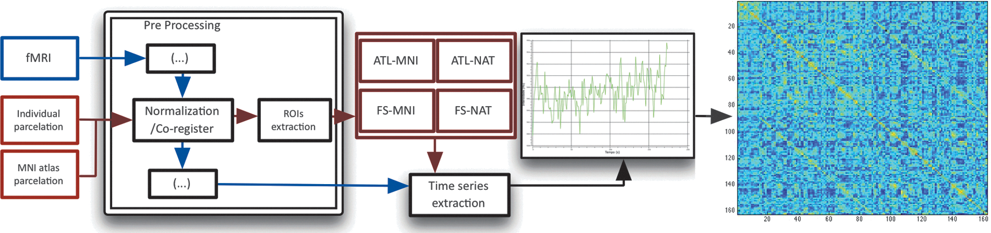
Complete image processing workflow: from the raw images to the correlation matrices. In blue, the workflow of functional images, and in red, the workflow of the node-defining atlases.

Network analysis and comparison

The comparison of the resulting networks was done at three levels: on the edges level, on the node level, and on the global network level. Regarding the networks' edges, differences in the Z-transformed correlation coefficients were tested for each pair of regions.

On the node level, two of the most commonly reported nodal metrics were used: betweenness centrality and local efficiency. The betweenness centrality, C_i ^B, measures the fraction of the shortest paths that pass through the node i of the network (Freeman, 1978): \documentclass{aastex}\usepackage{amsbsy}\usepackage{amsfonts}\usepackage{amssymb}\usepackage{bm}\usepackage{mathrsfs}\usepackage{pifont}\usepackage{stmaryrd}\usepackage{textcomp}\usepackage{portland,xspace}\usepackage{amsmath,amsxtra}\pagestyle{empty}\DeclareMathSizes{10}{9}{7}{6} \begin{document} \begin{align*}{ \rm C}_{ \rm i}^{ \rm B} = ( 1 / { \rm n} ( { \rm n} - 1 ) ) \sum \nolimits_{{ \rm s} \neq { \rm i} \neq { \rm t}} ( \sigma_{{ \rm st}} ( { \rm i} ) / \sigma_{{ \rm st}} )\end{align*} \end{document}

where σ_st(i) denotes the number of shortest paths between s and t that pass through i and σ_st denotes the total number of shortest paths between s and t. Measures of centrality evaluate the existence of nodes key to the communication of the network through which a significant number of communication paths go. Metrics of segregation indicate the existence of highly interconnected groups associated with functional specialization. Local efficiency (E_loc) is one of such metrics: \documentclass{aastex}\usepackage{amsbsy}\usepackage{amsfonts}\usepackage{amssymb}\usepackage{bm}\usepackage{mathrsfs}\usepackage{pifont}\usepackage{stmaryrd}\usepackage{textcomp}\usepackage{portland,xspace}\usepackage{amsmath,amsxtra}\pagestyle{empty}\DeclareMathSizes{10}{9}{7}{6} \begin{document} \begin{align*}{ \rm E}_{{ \rm loc}} = 1 / ( { \rm N} ) \sum \nolimits_{{ \rm i} \in { \rm N}} \left( \sum \nolimits_{{ \rm j , h \in N , j \neq i}}\ { \rm a}_{{ \rm ij}} { \rm a}_{{ \rm ih}}\ { \rm d}_{{ \rm ij}} ( { \rm N}_{ \rm i} ) ^{ - 1} \right) / { \rm k}_{{ \rm i}} ( { \rm k}_{{ \rm i}} - 1 )\end{align*} \end{document}

where N_i is the subgraph of the neighbors of node i, a_ij is the existence of a connection between i and j, and k_i is the degree of the node i.

On the network level, three properties were tested: clustering coefficient, average path length, and assortativity coefficient. As a measure of network segregation, the mean clustering coefficient C_p reflects the tendency to form clusters of interconnected nodes (Rubinov and Sporns, 2010; Watts and Strogatz, 1998): \documentclass{aastex}\usepackage{amsbsy}\usepackage{amsfonts}\usepackage{amssymb}\usepackage{bm}\usepackage{mathrsfs}\usepackage{pifont}\usepackage{stmaryrd}\usepackage{textcomp}\usepackage{portland,xspace}\usepackage{amsmath,amsxtra}\pagestyle{empty}\DeclareMathSizes{10}{9}{7}{6} \begin{document} \begin{align*}{ \rm C}_{ \rm p} = ( 1 / { \rm N} ) \sum { \rm C}_{ \rm i} , { \rm C}_{ \rm i} = ( { \rm e} ( { \rm G}_{ \rm i} )) / ( { \rm d} ( { \rm i} ) ( { \rm d} ( { \rm i} ) - 1 ) / 2)\end{align*} \end{document}

where N denotes the number of nodes in the network, C_i denotes the clustering coefficient of the node i in graph G, d(i) denotes the degree (or number of edges connected to) of the node i, and e(G_i) denotes the number of edges in G_i , the subgraph formed by all the node i neighbors. Functional integration measures reveal how easily each brain region communicates with the rest of the brain and combines specialized information. The average path length was used as a network-wise metric of integration, here calculated as the inverse of the network efficiency, E_glob , to allow its calculation in disconnected graphs (Latora and Marchiori, 2001; Rubinov and Sporns, 2010): \documentclass{aastex}\usepackage{amsbsy}\usepackage{amsfonts}\usepackage{amssymb}\usepackage{bm}\usepackage{mathrsfs}\usepackage{pifont}\usepackage{stmaryrd}\usepackage{textcomp}\usepackage{portland,xspace}\usepackage{amsmath,amsxtra}\pagestyle{empty}\DeclareMathSizes{10}{9}{7}{6} \begin{document} \begin{align*}{ \rm L} = 1 / { \rm E}_{{ \rm glob}} , { \rm E}_{{ \rm glob}} = 1 / ( { \rm N} ( { \rm N} - 1 ) ) \sum \nolimits_{{ \rm x , y \in G , x \neq y}}{ \rm d}_{{ \rm ij}}^{ - 1}\end{align*} \end{document}

where d_ij denotes the distance, or the minimum number of connections, between the nodes i and j. Measures of network resilience quantify the network's ability to resist direct or random attacks. One possible measure is the assortativity coefficient r, which measures the correlation between a node degree and the degree of its neighbors, in other words, shows how likely it is for a node with a high degree to be connected to nodes with a similar degree (Newman, 2002, 2003): \documentclass{aastex}\usepackage{amsbsy}\usepackage{amsfonts}\usepackage{amssymb}\usepackage{bm}\usepackage{mathrsfs}\usepackage{pifont}\usepackage{stmaryrd}\usepackage{textcomp}\usepackage{portland,xspace}\usepackage{amsmath,amsxtra}\pagestyle{empty}\DeclareMathSizes{10}{9}{7}{6} \begin{document} \begin{align*}{ \rm r} = \left( { \rm M}^{ - 1} \sum \nolimits_{{ \rm i} = 1.{ \rm M}} { \rm j}_{ \rm i}{ \rm k}_{ \rm i} - \left[ { \rm M}^{ - 1} \sum \nolimits_{{ \rm i} = 1.{ \rm M}} 1 / 2 ( { \rm j}_{ \rm i} + { \rm k}_{ \rm i} ) \right] ^2 \right) / \\ \left({ \rm M}^{ - 1} \sum \nolimits_{{ \rm i} = 1.{ \rm M}} 1 / 2 ( { \rm j}_{ \rm i} + { \rm k}_{ \rm i} ) - \left[ { \rm M}^{ - 1} \sum \nolimits_{{ \rm i} = 1.{ \rm M}} 1 / 2 ( { \rm j}_{ \rm i} +{ \rm k}_{ \rm i} ) \right] ^2 \right)\end{align*} \end{document}

M denotes the number of edges in the graph, j_i and k_i denote the degree of the nodes at both ends of the edge i.

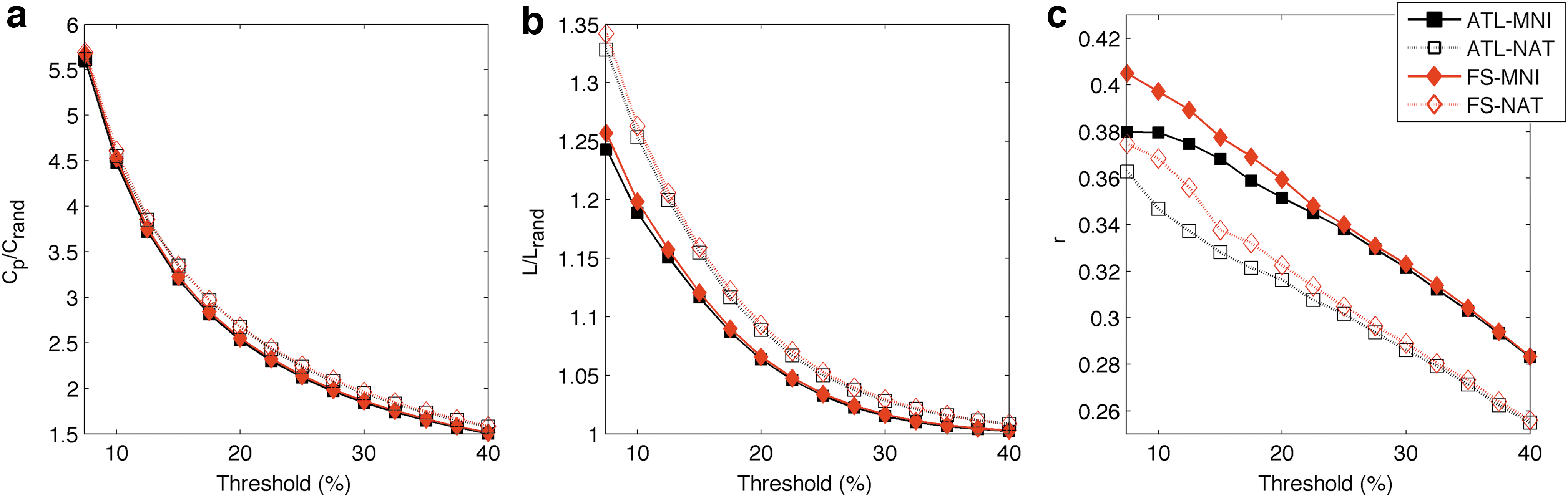
Commonly, networks can be classified according to different architectures. One such architecture is the small-world topology. These networks are usually defined as having a higher C_p than those found on random networks (C_p/C_{p rand} >1) and a similar L (L/L_rand ≈1) (Rubinov and Sporns, 2010; Watts and Strogatz, 1998). This translates into the formation of highly connected subnetworks while keeping a high level of connectivity (Sporns et al., 2004). As so, C_p/C_{p rand} and L/L_rand were also called small-world parameters and were used to characterize the networks.

The nodal and network metrics for all networks and subjects were calculated along a range of densities, from 5% to 40% in steps of 2.5%. To reduce the complexity of the analysis, the nodal properties were condensed across the density range through the use of the integrated version of the measure, calculated as follows (Tian et al., 2011): \documentclass{aastex}\usepackage{amsbsy}\usepackage{amsfonts}\usepackage{amssymb}\usepackage{bm}\usepackage{mathrsfs}\usepackage{pifont}\usepackage{stmaryrd}\usepackage{textcomp}\usepackage{portland,xspace}\usepackage{amsmath,amsxtra}\pagestyle{empty}\DeclareMathSizes{10}{9}{7}{6} \begin{document} \begin{align*}{ \rm X} ( { \rm i} ) = \sum \nolimits_{{ \rm i} = 5}{}^{{{ \rm k}} = 45}\ { \rm X} ( { \rm i; k \Delta d} ) \Delta { \rm d}\end{align*} \end{document}

where X is the property of the node i, along 15 density levels, and Δd is the density interval (0.025).

Only positive correlation coefficients were considered and all networks were binarized before calculation of the metrics. All calculations were done using the Brain Connectivity Toolbox (Rubinov and Sporns, 2010) and Matlab.

Statistical analysis

To compare the different strategies, a 2×2 repeated measures ANOVA was done using Matlab, on the Z-transformed correlation coefficients, metrics C^B, LocEf, C_p, L, r, and using the registration approach, parcellation strategy, and registration×parcellation interactions as within subject contrasts. The necessary assumptions for the analysis were previously verified and met. Differences were considered significant at p≤0.05 corrected for multiple comparisons using the family-wise error procedure.

Results

Network characterization

The average network matrices for each strategy, thresholded at a density of 7.5%, can be found in Figure 3. In these matrices, similar connection tendencies were observed for all the strategies. From the division in cortical and subcortical regions, it is possible to observe a tendency for stronger connections between regions of the same atlas; cortical regions revealed higher connectivity with other cortical regions than with subcortical regions and the same pattern was observed for subcortical regions. Moreover, regions tend to present stronger connections to regions within the same hemisphere than to regions of the contralateral hemisphere. A symmetry effect can also be observed, meaning that, regions showed strong tendencies to connect to the matching region on the contralateral hemisphere, as evidenced by the diagonal crossing both the second and third quadrant of the matrices (Fig. 3). From the distribution of Z-transformed correlation coefficients (Fig. 4a), it is possible to observe a roughly normal distribution with the majority of values located between 0 and 0.2, while in the distance distribution (Fig. 4b) it is noticeable that most values are located between 15 and 55 mm.

FIG. 3.

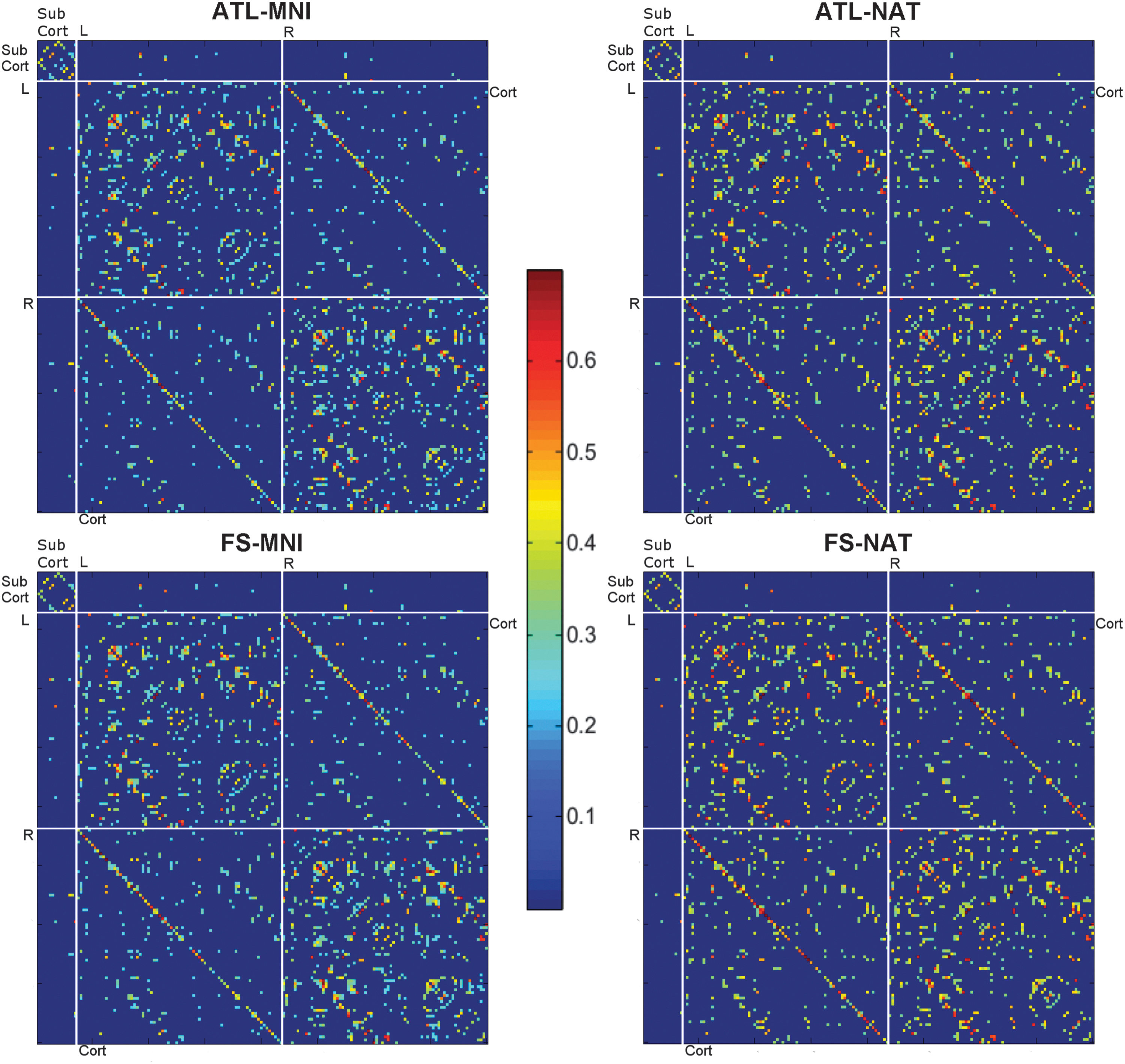
Correlation matrices for the four networks thresholded at 7.5% density averaged for all subjects: networks built using the presegmented atlas (ATL), the individual segmentation (FS), built on the standard MNI space, and on the functional native space (NAT). White lines divide the matrices in subcortical (SubCort) and cortical (Cort) regions as well as left and right. FS, FreeSurfer.

FIG. 4.

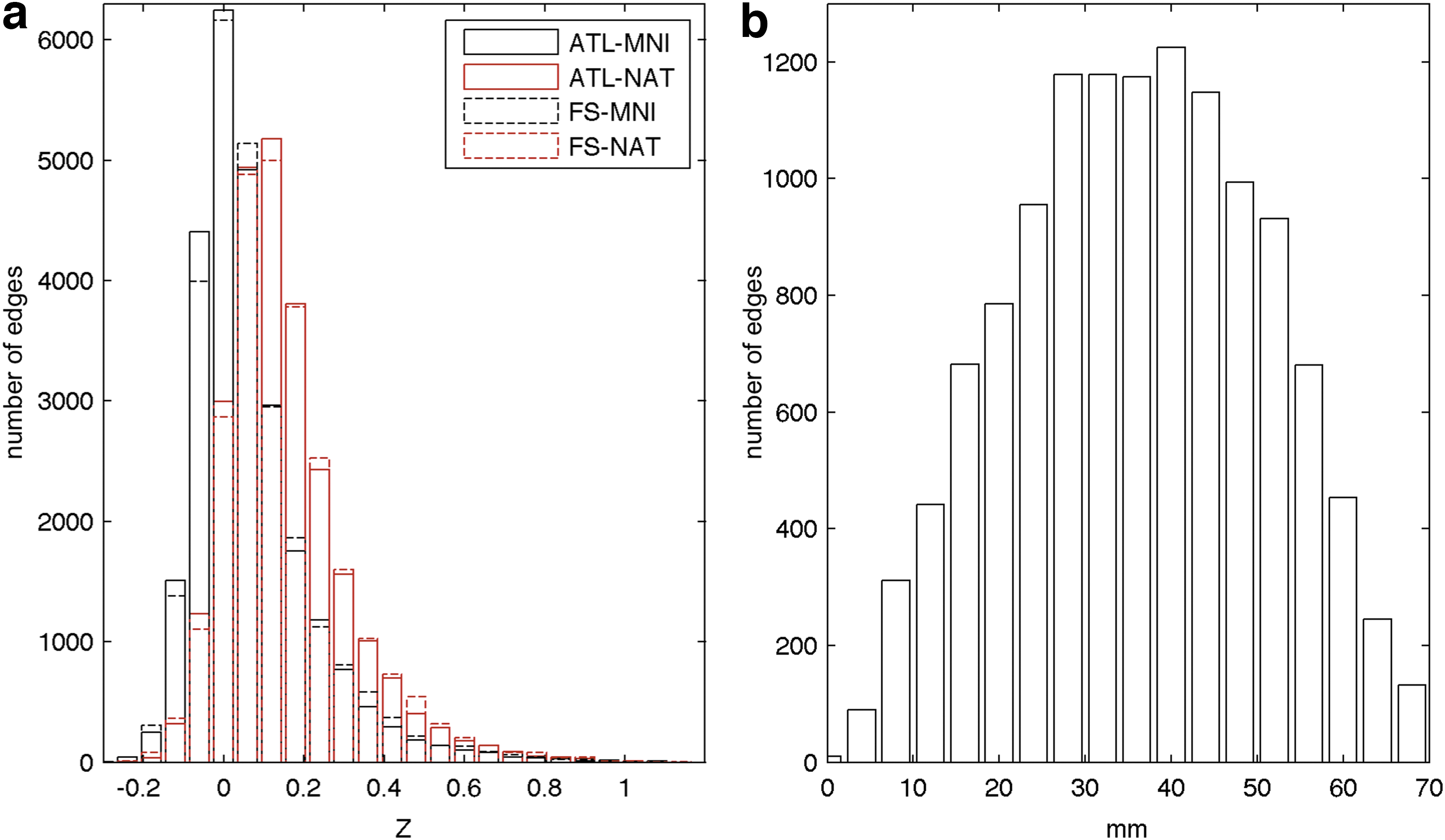
Networks distributions: (a) distribution of Z-transformed correlation values; (b) distribution of distances.

Regarding the small-world properties of the networks (Fig. 5), all presented high clustering values for the full range of densities, with 1.5<C_p/C_{p rand} <6, and a tendency for the values to become closer to those of random networks as the network density increased (Fig. 5a). The characterization of the average path length of each network revealed values close to those of random networks, with 1<L/L_rand <1.35, and once again a tendency to grow closer to those of random networks as the density increased (Fig. 5b). Concerning the assortativity of the networks, all values were found to be positive and 0.24<r<0.41 (Fig. 5c).

FIG. 5.

Global metrics network characterization. (a) C_p/C_prand, network average clustering coefficient compared to random networks; (b) L/L_rand, network average path length compared to random networks; (c) r, network assortativity. For the networks built using the presegmented atlas (ATL), the individual segmentation (FS), built on the standard MNI space (MNI), and on the functional native space (NAT).

Effect of registration and parcellation strategies

For the isolated effect of the registration and parcellation strategies, significant differences were found on the three levels of analysis.

In the edges comparison, differences were found in the registration test (Fig. 6a) in a total of 243 edges. All these edges, when computed in native space, presented higher values than the same edges computed in standard space. When considering the parcellation test (Fig. 6b), differences were found in a total of 112 edges, 26 of them having higher value on the ATL networks and 86 on the FS networks.

FIG. 6.

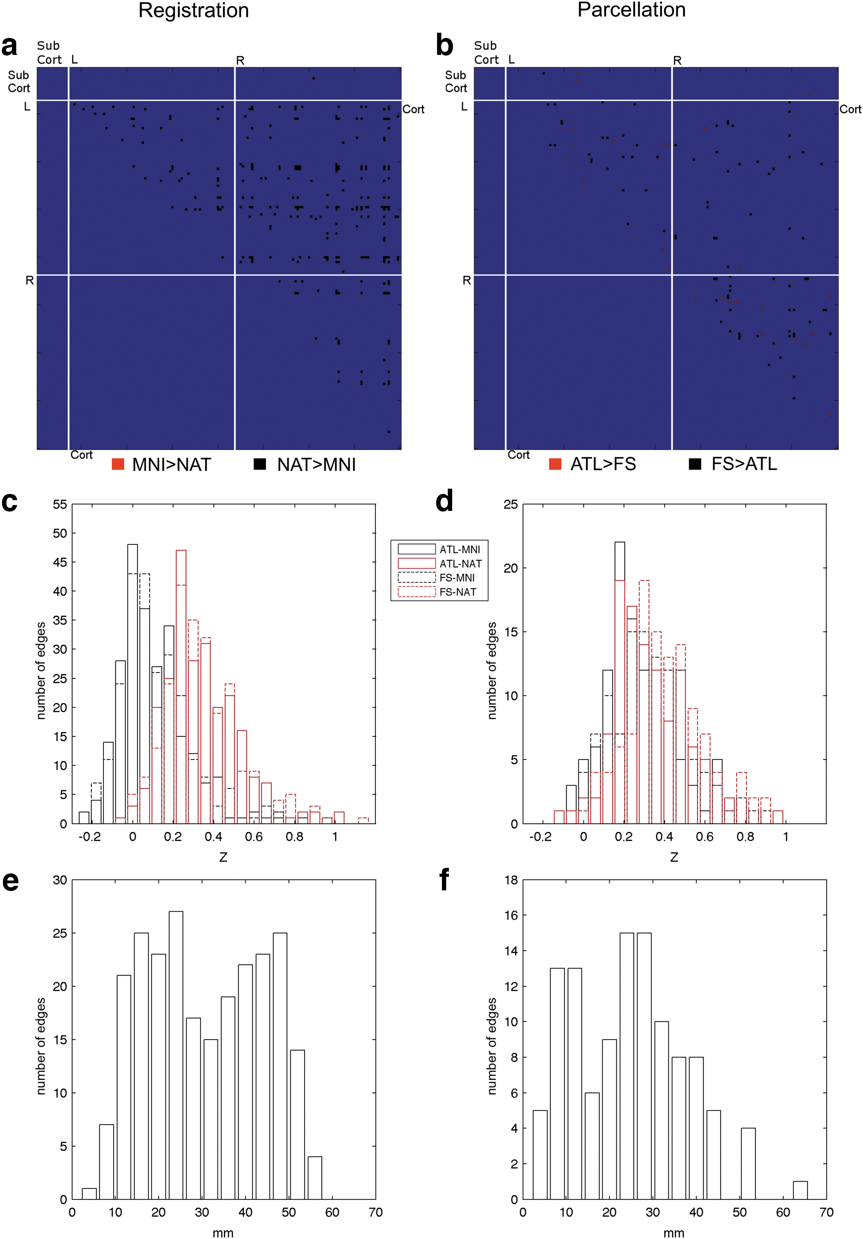
Edge level significant differences for the registration and parcellation comparisons for p<0.05 corrected for multiple comparisons with family-wise error procedure: (a, b) location and direction of differences; (c, d) distribution of the Z-transformed correlation values for the edges with significant differences for each network; (e, f) distribution of physical distances for the edges with significant differences.

From the distribution of correlations of the edges with significant differences on the registration comparison (Fig. 6c), it was possible to observe that the NAT networks Z-transformed correlation values lie between 0.2 and 0.4, while on the MNI networks these were mainly located between −0.1 and 0.2. On the parcellation comparison (Fig. 6d), the values of Z-transformed correlation with significant differences from all networks were located mainly between 0.2 and 0.4. From the distance distribution of differences on the registration comparison (Fig. 6e), it was possible to observe a tendency for differences to be located on either long- or short-distance edges with a higher tendency for the short range. On the parcellation comparison, differences were mainly located over shorter connections (Fig. 6f).

On the nodal metrics, differences were found on both metrics for the registration test: one on C^B, with MNI networks having a higher value, and five on the E_loc, with the NAT networks always having higher values. On the parcellation test, significant differences were found on the C^B metric on three vertices with FS networks always having higher values and no differences were found on the E_loc (Table 2).

Table 2.

Significant Differences in the Nodal Metrics in Bold for the Registration and Parcellation Comparisons

	Networks				Registration		Parcellation
	ATL-MNI	ATL-NAT	FS-MNI	FS-NAT	F_(1,54)	η_p ²	F_(1,54)	η_p ²
Node	C^B
Left-Pole_temporal	59.554	62.079	76.751	79.507	0.178	0.003	23.840	0.310
Right-Gand_S_occipital_inf	53.345	55.552	68.158	79.448	1.085	0.020	16.988	0.243
Right-Lat_Fis-ant-Horizont	60.639	33.838	57.997	38.138	18.769	0.262	0.068	0.001
Right-Pole_temporal	72.203	67.579	83.074	82.113	0.251	0.005	15.260	0.224
	E_loc
Left-S_postcentral	0.272	0.287	0.275	0.291	18.358	0.257	1.857	0.034
Right-G_and_S_cingul-Mid-Post	0.257	0.280	0.259	0.282	22.277	0.296	0.279	0.005
Left-G_postcentral	0.272	0.285	0.270	0.290	20.098	0.275	0.717	0.013
RightS_postcentral	0.272	0.290	0.274	0.293	22.781	0.301	1.079	0.020
Right-S_precentral-sup-part	0.255	0.276	0.259	0.286	14.980	0.220	5.514	0.094

p<0.05 corrected for multiple comparisons with the family-wise error procedure.

ATL, atlas; FS, FreeSurfer; MNI, Montreal National Institute; NAT, native.

On the global metrics level, several differences were found as follows: on the registration test, differences were found on the clustering metric for values of density between 15% and 40%, with the NAT networks always having higher values; on the average path length, differences were found on the full range of densities, with the NAT networks having higher values; and no differences were found on the assortativity metric (Table 3).

Table 3.

Isolated Effect of the Registration Strategies for the Graph Metrics Across All Threshold Values

	C_p: NAT>MNI			L: NAT>MNI			r: MNI>NAT
Thresho ld (%)	p	F_(1,54)	η_p ²	p	F_(1,54)	η_p ²	p	F_(1,54)	η_p ²
5	0.170	1.931	0.035	<0.001	19.687	0.271	0.384	0.770	0.014
7.5	0.659	0.197	0.004	<0.001	20.309	0.277	0.153	2.099	0.038
10	0.094	2.905	0.052	<0.001	21.534	0.289	0.050	4.034	0.071
12.5	0.003	9.927	0.158	<0.001	21.910	0.292	0.018	6.010	0.102
15	<0.001	15.641	0.228	<0.001	23.712	0.309	0.004	9.018	0.145
17.5	<0.001	19.974	0.274	<0.001	23.474	0.307	0.004	8.932	0.144
20	<0.001	22.796	0.301	<0.001	25.725	0.327	0.005	8.713	0.141
22.5	<0.001	23.307	0.305	<0.001	26.208	0.331	0.004	9.336	0.150
25	<0.001	24.921	0.320	<0.001	26.813	0.336	0.003	9.803	0.156
27.5	<0.001	25.762	0.327	<0.001	28.240	0.348	0.003	9.906	0.157
30	<0.001	27.324	0.340	<0.001	28.841	0.352	0.003	9.986	0.159
32.5	<0.001	27.182	0.339	<0.001	29.586	0.358	0.003	9.624	0.154
35	<0.001	27.413	0.341	<0.001	28.214	0.347	0.006	8.305	0.135
37.5	<0.001	28.458	0.349	<0.001	26.104	0.330	0.008	7.728	0.127
40	<0.001	29.942	0.361	<0.001	24.315	0.314	0.014	6.421	0.108

Significant results in bold corrected for multiple comparisons with the family-wise error procedure.

For the parcellation test, differences were found for the clustering coefficient between densities of 22.5% and 40%, on the average path length for density values of 5%, 17.5%, and 20%, and on the assortativity metric, a density of 12.5%. In all instances, FS networks showed higher values than ATL networks (Table 4).

Table 4.

Isolated Effect of the Parcellation Strategies for the Graph Metrics Across All Threshold Values

	C_p: FS>ATL			L: FS>ATL			r: FS>ATL
Threshold (%)	p	F_(1,54)	η_p ²	p	F_(1,54)	η_p ²	p	F_(1,54)	η_p ²
5	0.58	0.31	0.006	<0.001	15.107	0.222	0.005	8.721	0.141
7.5	0.015	6.29	0.106	0.002	11.028	0.172	0.006	8.373	0.136
10	0.008	7.604	0.125	0.002	10.404	0.164	0.001	13.110	0.198
12.5	0.165	1.984	0.036	0.002	10.131	0.160	0.000	15.192	0.223
15	0.067	3.485	0.062	0.003	9.614	0.154	0.008	7.639	0.126
17.5	0.016	6.159	0.104	<0.001	19.658	0.271	0.003	9.782	0.156
20	0.038	4.514	0.078	<0.001	14.613	0.216	0.040	4.440	0.077
22.5	<0.001	13.808	0.207	0.002	10.568	0.166	0.166	1.969	0.036
25	<0.001	19.346	0.267	0.002	10.783	0.169	0.403	0.710	0.013
27.5	<0.001	21.622	0.290	0.005	8.533	0.139	0.498	0.467	0.009
30	<0.001	28.434	0.349	0.009	7.348	0.122	0.482	0.502	0.009
32.5	<0.001	29.846	0.360	0.016	6.228	0.105	0.656	0.200	0.004
35	<0.001	29.312	0.356	0.045	4.202	0.073	0.592	0.290	0.005
37.5	<0.001	25.243	0.323	0.181	1.839	0.034	0.694	0.157	0.003
40	<0.001	25.713	0.327	0.119	2.505	0.045	0.781	0.078	0.001

Significant results in bold corrected for multiple comparisons with the family-wise error procedure.

Interactions between the node definition and registration strategies

No significant results were found for the registration×parcellation interaction.

Discussion

The results herein obtained are in accordance to the expected characteristics and architecture of brain networks, as demonstrated in several studies (Braun et al., 2012; Messé et al., 2012; Tian et al., 2011; van Wijk et al., 2010; Wang et al., 2009). All networks were shown to be assortative (r>0) and efficient (L/L_rand ≈1) in the full range of densities. All of them also showed a strong small-world-like tendency to constitute clusters (C_p /C_{p rand} >1) on the lower range of densities (5% to 20%).

The thresholded correlation matrices demonstrated a clear tendency for regions to connect to other regions within the same anatomical division (cortical/subcortical and left/right), evidencing not only a tendency for lateralization of function in the human brain (Tian et al., 2011) but also reflecting a tendency to have more efficient networks by having stronger connections over smaller anatomical distances (Tomasi and Volkow, 2012). The diagonals over the L/R quadrants reflect the natural correlation and sharing of functions between symmetric regions (Salvador et al., 2005; Toro et al., 2008).

For the isolated effect of the registration strategies, several significant differences were found in all three levels of the analysis. From the differences matrix and the corresponding correlation and distance distribution, it is possible to observe a strong tendency for the networks built in the functional native space to have higher values of correlation and for these differences to be mainly located on either shorter or longer range connections. These differences translate in the network metrics into a higher clustering coefficient and longer average path distance in the native space networks with a very large effect size (Cohen, 1988). Overall, this seems to point that networks built in this space favor the detection of stronger local paths of communication, not restrained to physically proximal or interhemispheric regions, in detriment of more evenly spread connections. On the nodal metrics, it could be expected that this would translate into a higher tendency for the native space networks to have vertices with a stronger centrality role. Instead, the authors found differences in only one vertex in B^C, favoring the MNI space networks (although with a small effect size). In the local efficiency, the differences favor again the native space networks, with the existence of nodes with a more important role on facilitating the communication on their local networks, which should be associated with the higher clustering coefficient, but again, with a small effect size. The differences found can be the result of multiple factors: the resampling and interpolation of the functional data in the normalization step, the resampling of the parcellation images and loss of detail, or a mixture of both. As no interaction was found between the registration and parcellation strategies, the first option emerges as the most likely.

In the parcellation strategies comparison, several differences were also found. At the correlation level it is possible to observe differences in both directions, mostly with higher values in the individual segmentation networks. From the correlation distribution, it is possible to observe a small tendency for the individual segmentation networks to have higher values of correlation, and from the distance distribution, for the differences to be located mainly over shorter range edges and within hemispheres. The authors found higher values of C_p in the individual segmentation strategies, with large to very large effect sizes, L, with high effect sizes, C^B, with small to very small effect sizes, and r with large effect sizes. These differences can be explained by the higher precision of the strategy in segmenting the different areas according to sulci and gyri (Destrieux et al., 2010), possibly establishing higher and more accurate correlations. This strategy seems to favor the detection of strong and short connections associated with the formation of local clusters (as seen in the increased C_p). The lack of the ability of the fixed template strategy networks to detect these strong correlations favors the survival on the threshold procedure of the weaker long-distance connections, establishing extra paths of communication between distant points in the network and reducing the average shortest path in these networks. Furthermore, on the nodal metrics comparison, three individual segmentation network vertices were found to have a higher value of B^C. As the main hubs of communication in a network are usually associated with the necessity to establish bridges of communications between strong and independent clusters, these seem to be a logical finding, supported by the large effect size.

This study presents some limitations that should be noted. While the authors reveal the impact of the normalization step in several aspects of the network, it is, in this study, impossible to show which inner step of the normalization is the exact step responsible for these differences. Further exploration of the effect of resampling the functional data and the use of different interpolation functions are needed to characterize the exact effect of this step. It is also important to notice that several of the differences found in the network metrics were present on higher values of density. This can be explained by observing the distributions of correlations of differences, as most edges with significant differences have medium to low levels of correlation, and only once these survive the thresholding procedure their effect will be noticeable on the network. There is a tendency in neuroimaging studies to focus on lower density networks, possibly reducing the relevance of some of the present findings. Yet, there is no direct evidence of which density threshold is more appropriate, which could be critical for the overall interpretation of the present finding and of complex brain networks studies.

Overall, the authors have shown a strong impact of two different preprocessing steps on the resulting networks. It is, without prior knowledge of the expected network properties, impossible to determine which strategy better represents the underlying biological brain network, making it only possible to theoretically argue in favor of those strategies that have either less impact on the data or are more precise in defining the ROIs. While further exploration of the normalization step is needed, the present results favor the use of the more conservative approach, avoiding the use of resampling and interpolation functions on the data whenever possible. Similar to this, the use of a more precise segmentation method for defining the ROIs also seems to have a moderate impact on the networks obtained.

Footnotes

Acknowledgments

The authors are thankful to all the study participants.

Financial Disclosures: R.M. is supported by a fellowship of the project FCT-ANR/NEU-OSD/0258/2012 founded by FCT/MEC (www.fct.pt) and by Fundo Europeu de Desenvolvimento Regional (FEDER). PM was supported by a fellowship of the project SwitchBox-FP7-HEALTH-2010-grant 259772-2 (www.switchbox-online.eu). The funders had no role in the study design, data collection and analysis, decision to publish, or preparation of the manuscript.

Author Disclosure Statement

No competing financial interests exist.

References

Achard

, Bullmore

. 2007. Efficiency and cost of economical brain functional networks. PLoS Comput Biol, 3:e17.

Achard

, Salvador

, Whitcher

, Suckling

, Bullmore

. 2006. A resilient, low-frequency, small-world human brain functional network with highly connected association cortical hubs. J Neurosci, 26:63–72.

Behzadi

, Restom

, Liau

, Liu

. 2007. A component based noise correction method (CompCor) for BOLD and perfusion based fMRI. Neuroimage, 37:90–101.

Braun

, Plichta

, Esslinger

, Sauer

, Haddad

, et al. 2012. Test-retest reliability of resting-state connectivity network characteristics using fMRI and graph theoretical measures. Neuroimage, 59:1404–1412.

Bullmore

, Sporns

. 2009. Complex brain networks: graph theoretical analysis of structural and functional systems. Nat Rev Neurosci, 10:186–198.

Bullmore

, Bassett

. 2011. Brain graphs: graphical models of the human brain connectome. Annu Rev Clin Psychol, 7:113–140.

Cohen

. 1988. Statistical Power Analysis for the Behavioral Sciences. Hillsdale, NJ: Psychology Press.

Destrieux

, Fischl

, Dale

, Halgren

. 2010. Automatic parcellation of human cortical gyri and sulci using standard anatomical nomenclature. Neuroimage, 53:1–15.

Felleman

, Van Essen

. 1991. Distributed hierarchical processing in the primate cerebral cortex. Cereb Cortex, 1:1–47.

10.

Fischl

. 2012. FreeSurfer. Neuroimage, 62:774–781.

11.

Fischl

, Salat

, Busa

, Albert

, Dieterich

, et al. 2002. Whole brain segmentation: automated labeling of neuroanatomical structures in the human brain. Neuron, 33:341–355.

12.

Freeman

. 1978. Centrality in social networks conceptual clarification. Soc Netw, 1:215–239.

13.

Gross

, Yellen

. 2006. Graph Theory and Its Applications. Boca Raton, FL: Chapman & Hall/CRC.

14.

Hagmann

, Kurant

, Gigandet

, Thiran

, Wedeen

, et al. 2007. Mapping human whole-brain structural networks with diffusion MRI. PLoS One, 2:e597.

15.

, Evans

. 2010. Graph theoretical modeling of brain connectivity. Curr Opin Neurol, 23:341–350.

16.

Hosseini

, Kesler

. 2013. Comparing connectivity pattern and small-world organization between structural correlation and resting-state networks in healthy adults. Neuroimage, 78:402–414.

17.

Huang

, Li

, Sun

, Ye

, Fleisher

, et al. 2010. Learning brain connectivity of Alzheimer's disease by sparse inverse covariance estimation. Neuroimage, 50:935–949.

18.

Jenkinson

, Smith

. 2001. A global optimisation method for robust affine registration of brain images. Med Image Anal, 5:143–156.

19.

Lang

, Tome

, Keck

, Gorriz-Saez

, Puntonet

. 2012. Brain connectivity analysis: a short survey. Comput Intell Neurosci, 2012:412512.

20.

Latora

, Marchiori

. 2001. Efficient behavior of small-world networks. Phys Rev Lett, 87:198701.

21.

Liang

, Wang

, Yan

, Shu

, Xu

, et al. 2012. Effects of different correlation metrics and preprocessing factors on small-world brain functional networks: a resting-state functional MRI study. PLoS One, 7:e32766.

22.

Lord

, Allen

, Expert

, Howes

, Lambiotte

, et al. 2011. Characterization of the anterior cingulate's role in the at-risk mental state using graph theory. Neuroimage, 56:1531–1539.

23.

Marques

, Soares

, Alves

, Sousa

. 2013. BrainCAT—a tool for automated and combined functional magnetic resonance imaging and diffusion tensor imaging brain connectivity analysis. Front Hum Neurosci, 7:794.

24.

Mazziotta

, Toga

, Evans

, Fox

, Lancaster

, et al. 2001. A four-dimensional probabilistic atlas of the human brain. J Am Med Inform Assoc, 8:401–430.

25.

McIntosh

, Nyberg

, Bookstein

, Tulving

. 1997. Differential functional connectivity of prefrontal and medial temporal cortices during episodic memory retrieval. Hum Brain Mapp, 5:323–327.

26.

McIntosh

, Rajah

, Lobaugh

. 1999. Interactions of prefrontal cortex in relation to awareness in sensory learning. Science, 284:1531–1533.

27.

Messé

, Marrelec

, Bellec

, Perlbarg

, Doyon

, et al. 2012. Comparing structural and functional graph theory features in the human brain using multimodal MRI. IRBM, 33:244–253.

28.

Minati

, Grisoli

, Seth

, Critchley

. 2012. Decision-making under risk: a graph-based network analysis using functional MRI. Neuroimage, 60:2191–2205.

29.

Newman

MEJ

. 2002. Assortative mixing in networks. Phys Rev Lett, 89:208701.

30.

Newman

MEJ

. 2003. The structure and function of complex networks. SIAM Rev, 45:167–256.

31.

Ogawa

, Lee

, Kay

, Tank

. 1990. Brain magnetic resonance imaging with contrast dependent on blood oxygenation. Proc Natl Acad Sci U S A, 87:9868–9872.

32.

Richiardi

, Eryilmaz

, Schwartz

, Vuilleumier

, Van De Ville

. 2011. Decoding brain states from fMRI connectivity graphs. Neuroimage, 56:616–626.

33.

Rubinov

, Sporns

. 2010. Complex network measures of brain connectivity: uses and interpretations. Neuroimage, 52:1059–1069.

34.

Salvador

, Suckling

, Coleman

, Pickard

, Menon

, et al. 2005. Neurophysiological architecture of functional magnetic resonance images of human brain. Cereb Cortex, 15:1332–1342.

35.

Sporns

. 2012. From simple graphs to the connectome: networks in neuroimaging. Neuroimage, 62:881–886.

36.

Sporns

, Chialvo

, Kaiser

, Hilgetag

. 2004. Organization, development and function of complex brain networks. Trends Cogn Sci, 8:418–425.

37.

Sporns

, Tononi

, Edelman

. 1991. Modeling perceptual grouping and figure-ground segregation by means of active reentrant connections. Proc Natl Acad Sci U S A, 88:129–133.

38.

Stam

, Reijneveld

. 2007. Graph theoretical analysis of complex networks in the brain. Nonlinear Biomed Phys, 1:3.

39.

Sun

, Hu

, Huang

, Liu

, Li

, et al. 2012. Inferring consistent functional interaction patterns from natural stimulus FMRI data. Neuroimage, 61:987–999.

40.

Supekar

, Musen

, Menon

. 2009. Development of large-scale functional brain networks in children. PLoS Biol, 7:e1000157.

41.

Tian

, Wang

, Yan

, He

. 2011. Hemisphere- and gender-related differences in small-world brain networks: a resting-state functional MRI study. Neuroimage, 54:191–202.

42.

Tomasi

, Volkow

. 2012. Laterality patterns of brain functional connectivity: gender effects. Cereb Cortex, 22:1455–1462.

43.

Toro

, Fox

, Paus

. 2008. Functional coactivation map of the human brain. Cereb Cortex, 18:2553–2559.

44.

van den Heuvel

, Stam

, Boersma

, Hulshoff Pol

. 2008. Small-world and scale-free organization of voxel-based resting-state functional connectivity in the human brain. Neuroimage, 43:528–539.

45.

van Wijk

, Stam

, Daffertshofer

. 2010. Comparing brain networks of different size and connectivity density using graph theory. PLoS One, 5:e13701.

46.

Vandenberghe

, Wang

, Nelissen

, Vandenbulcke

, Dhollander

, et al. 2013. The associative-semantic network for words and pictures: effective connectivity and graph analysis. Brain Lang, 127:264–272.

47.

Wang

, Wang

, Zang

, Yang

, Tang

, et al. 2009. Parcellation-dependent small-world brain functional networks: a resting-state fMRI study. Hum Brain Mapp, 30:1511–1523.

48.

Watts

, Strogatz

. 1998. Collective dynamics of ‘small-world’ networks. Nature, 393:440–442.

49.

Whitfield-Gabrieli

, Nieto-Castanon

. 2012. Conn: a functional connectivity toolbox for correlated and anticorrelated brain networks. Brain Connect, 2:125–141.

50.

Young

. 1992. Objective analysis of the topological organization of the primate cortical visual system. Nature, 358:152–155.

51.

, Huang

, Singer

, Nikolic

. 2008. A small world of neuronal synchrony. Cereb Cortex, 18:2891–2901.