The Union of Shortest Path Trees of Functional Brain Networks

Abstract

Communication between brain regions is still insufficiently understood. Applying concepts from network science has shown to be successful in gaining insight in the functioning of the brain. Recent work has implicated that especially shortest paths in the structural brain network seem to play a major role in the communication within the brain. So far, for the functional brain network, only the average length of the shortest paths has been analyzed. In this article, we propose to construct the union of shortest path trees (USPT) as a new topology for the functional brain network. The minimum spanning tree, which has been successful in a lot of recent studies to comprise important features of the functional brain network, is always included in the USPT. After interpreting the link weights of the functional brain network as communication probabilities, the USPT of this network can be uniquely defined. Using data from magnetoencephalography, we applied the USPT as a method to find differences in the network topology of multiple sclerosis patients and healthy controls. The new concept of the USPT of the functional brain network also allows interesting interpretations and may represent the highways of the brain.

Introduction

Analyzing the brain as a complex network has become an often used approach in modern neuroscience and has led to new insights concerning brain disorders (Bullmore and Sporns, 2009, 2012). Recently, the shortest paths between brain regions were found to be crucial to understand functional networks in terms of structural networks (Goñi et al., 2014) and pathological network alterations in brain diseases. Structural or functional brain networks in patients with neuropsychiatric diseases are often characterized by a reduced global efficiency, which is proportional to the inverse of the shortest paths. However, the shortest paths of the functional brain network have merely been analyzed with regard to their average length. Using all shortest paths as an alternative topology for the functional brain network is a new approach.

Several sampling methods on functional brain networks set a threshold or fix the link density to thin the complete weighted graph. However, these methods have disadvantages: the choice of the a priori chosen threshold or link density is often arbitrary and, in addition, different link densities can lead to different results (van Wijk et al., 2010). Constructing the minimum spanning tree (MST) of the functional brain network has provided insight in the differences between patients suffering from brain disorders and healthy controls in a lot of recent studies (Dubbelink et al., 2014; Stam et al., 2014; Tewarie et al., 2014; van Dellen et al., 2014; Wang et al., 2010). An advantage of the MST lies in its independence of the transformation of the weights as long as their ranking is unaltered. There exists only one unique path from a node to another node in the MST, which limits more advanced analysis.

Analyzing shortest paths is a common practice after reducing the complete graph of the functional brain network with any of the existing sampling methods. Bullmore and Sporns (2012) suggested that the brain is always trying to reduce material and metabolic costs when transporting information. Thus, the concept of shortest paths fits into the current understanding of the brain function. Extracting all shortest paths of the original complete graph can be interpreted as focusing on the backbone or the main functional highways of the brain network. We intend to represent the most important connections of the functional brain network based on global network properties and not only on the ranking of the link weights among each other.

In the present study, we propose the union of shortest path trees (USPT) as a new sampling method for the functional brain network. This sampling method has been successfully applied before on a variety of complex networks (Van Mieghem and Wang, 2009). To construct the USPT, we first identify the shortest path tree rooted at each node in the network. The shortest path tree rooted at a node consists of all shortest paths from this node to all the other nodes (Van Mieghem and Magdalena, 2005). The union of all shortest paths from a single node to the rest of the network always results in a tree (Van Mieghem, 2011b). Furthermore, we can unite these shortest path trees to obtain the USPT G_{∪_SPT} of our network G (Van Mieghem and Wang, 2009). The USPT is determined by the topology of the underlying network and its link weight structure (the set of weights on the links in G) (Van Mieghem and Wang, 2009). Furthermore, if all link weights equal 1, the USPT is the same as the underlying network because all information then flows over the direct pathways between the nodes.

The properties of the USPT have been analyzed in various studies (Van Mieghem and Magdalena, 2005; Van Mieghem and Wang, 2009). The USPT, not the underlying network, determines the network's performance (Van Mieghem and Wang, 2009). Another important property of the USPT is that it always includes the MST (Van Mieghem and Wang, 2009) (Fig. 1). The regime, where the USPT coincides with the MST is called the strong disorder regime, the counterpart is the weak disorder regime (Van Mieghem and Magdalena, 2005; Van Mieghem and van Langen, 2005). In the strong disorder regime, all traffic in the network follows only links in the MST, while in the weak disorder regime, a transport may follow other paths. Analogous to the flow of electrical current, we may regard the strong disorder regime as the superconductive phase, whereas the weak disorder corresponds to the resistive phase, where electrons follow many paths between two different voltage points.

FIG. 1.

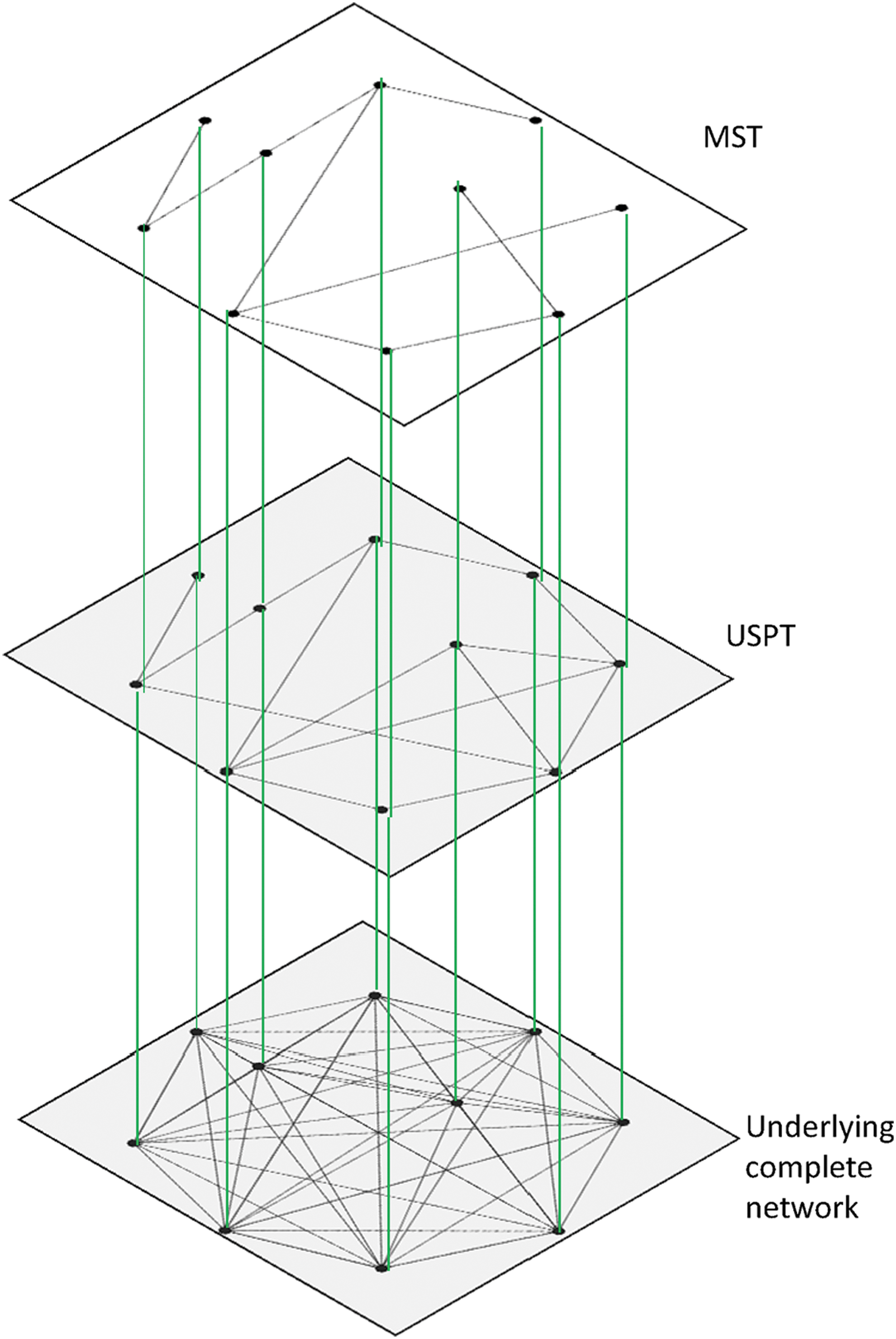
Visualization of a complete network with its corresponding USPT and MST. MST, minimum spanning tree; USPT, union of shortest path trees. Color images available online at www.liebertpub.com/brain

In many real-world networks, the information is assumed to flow over the shortest path to optimize transportation costs. The derivation of G_{∪_SPT} can be regarded as a filter for the weights that are not important for the overall transportation flow in the brain. By reducing the network to the union of its shortest paths, only those paths are maintained that have a high probability that information is transported along them. The topology of G_{∪_SPT} represents the highways of the brain. The goal of this article is to evaluate and apply this USPT sampling method to the functional brain network and to find first differences between patients and healthy controls.

In the following, we will interpret the link weights of the functional brain network as communication probabilities and, based on this interpretation, we will construct and analyze the USPT. We will examine the results of this new USPT sampling method by using empirical data from healthy controls and multiple sclerosis (MS) patients and demonstrate that the USPT is sensitive to disease alterations and that our USPT method can be used to discriminate between healthy and pathological conditions.

Materials and Methods

Data acquisition

In this section, we explain the reconstruction of functional brain networks from our magnetoencephalography (MEG) measurements. Our data set consisted of 68 healthy controls and 111 MS patients, which is a larger but overlapping group as in Tewarie and associates (2014, 2015). Details with regard to data acquisition and postprocessing can be found in our previous article (Tewarie et al., 2014). In short, MEG data were recorded using a 306-channel whole-head MEG system (ElektaNeuromag, Oy, Helsinki, Finland). Fluctuations in magnetic field strength were recorded during a no-task eyes-closed condition for 5 consecutive minutes. A beamformer approach was adopted to project MEG data from sensor space to source space (Hillebrand et al., 2012). This beamformer approach can be regarded as a spatial filter that computes the activity within brain regions based on the weighted sum of the activity recorded at the MEG channels. We then used the automated anatomical labeling atlas to obtain time series for 78 cortical regions of interest (ROIs) (Gong et al., 2009; Tzourio-Mazoyer et al., 2002). For each subject, we chose five artifact-free epochs of source space time series (Dubbelink et al., 2014; Tewarie et al., 2014; van Dellen et al., 2014). Six frequency bands were analyzed: delta (0.5–4 Hz), theta (4–8 Hz), lower alpha (8–10 Hz), upper alpha (10–13 Hz), beta (13–30 Hz), and lower gamma bands (30–48 Hz).

Subsequently, for each epoch and frequency band separately, we computed the phase lag index (PLI) between all time series of the 78 ROIs to obtain the link weights for our functional brain networks (Stam and Van Straaten, 2012; Stam et al., 2007). The PLI can take values between 0 and 1 and is a measure that captures phase synchronization by calculating the asymmetry of the distribution of instantaneous phase differences between time series. Formally, the PLI is defined as \documentclass{aastex}\usepackage{amsbsy}\usepackage{amsfonts}\usepackage{amssymb}\usepackage{bm}\usepackage{mathrsfs}\usepackage{pifont}\usepackage{stmaryrd}\usepackage{textcomp}\usepackage{portland, xspace}\usepackage{amsmath, amsxtra}\pagestyle{empty}\DeclareMathSizes{10}{9}{7}{6}\begin{document} \begin{align*} {\rm PLI} = \mid \langle {\rm sign} [{\rm sin} (\Delta \phi(t_{k}))] \rangle \mid \tag {1} \end{align*} \end{document}

where ΔΦ(t_k ), for k=1, …, m; \documentclass{aastex}\usepackage{amsbsy}\usepackage{amsfonts}\usepackage{amssymb}\usepackage{bm}\usepackage{mathrsfs}\usepackage{pifont}\usepackage{stmaryrd}\usepackage{textcomp}\usepackage{portland, xspace}\usepackage{amsmath, amsxtra}\pagestyle{empty}\DeclareMathSizes{10}{9}{7}{6}\begin{document}$$m \ \in \ \mathbb{N}$$ \end{document} , is the time series of phase differences evaluated for time steps t ₁ , …, t_m , \documentclass{aastex}\usepackage{amsbsy}\usepackage{amsfonts}\usepackage{amssymb}\usepackage{bm}\usepackage{mathrsfs}\usepackage{pifont}\usepackage{stmaryrd}\usepackage{textcomp}\usepackage{portland, xspace}\usepackage{amsmath, amsxtra}\pagestyle{empty}\DeclareMathSizes{10}{9}{7}{6}\begin{document}$$\langle . \rangle$$ \end{document} denotes the average, and \documentclass{aastex}\usepackage{amsbsy}\usepackage{amsfonts}\usepackage{amssymb}\usepackage{bm}\usepackage{mathrsfs}\usepackage{pifont}\usepackage{stmaryrd}\usepackage{textcomp}\usepackage{portland, xspace}\usepackage{amsmath, amsxtra}\pagestyle{empty}\DeclareMathSizes{10}{9}{7}{6}\begin{document}$$\mid . \mid$$ \end{document} the absolute value. High values of the PLI refer to a strong interaction or synchronization between two time series while avoiding bias due to volume conduction.

As a next step, for each epoch, we constructed an N x N weight matrix W with elements w_ij , each representing the PLI of the pair of regions, i and j. This symmetric weight matrix W can be interpreted as a complete weighted graph on N nodes (N=78). Last, we averaged over all five weight matrices belonging to each epoch to obtain one weight matrix per person and to ensure independent samples for statistical testing. All further mentioned weight matrices in this article refer to matrices with PLI values as entries.

Link weights in functional brain networks as communication probabilities

A network can be represented by a graph G consisting of N nodes and L links. Each link l=i→j from node i to j in G can be specified by a link weight w_l =w_ij =w(i→j). Assume a path from a node A to node B in our network G. We denote this path by P_A→B =n ₁ n ₂ ..n_k− ₁ n_k with hopcount (sometimes also called the length) \documentclass{aastex}\usepackage{amsbsy}\usepackage{amsfonts}\usepackage{amssymb}\usepackage{bm}\usepackage{mathrsfs}\usepackage{pifont}\usepackage{stmaryrd}\usepackage{textcomp}\usepackage{portland, xspace}\usepackage{amsmath, amsxtra}\pagestyle{empty}\DeclareMathSizes{10}{9}{7}{6}\begin{document}$$k \in {\mathbb N}$$ \end{document} , where n ₁=A, n_k =B, and n ₂ ,…, n_k− ₁ represent the distinct nodes along the path (Van Mieghem, 2014). The weight of a path P_A→B is usually defined as \documentclass{aastex}\usepackage{amsbsy}\usepackage{amsfonts}\usepackage{amssymb}\usepackage{bm}\usepackage{mathrsfs}\usepackage{pifont}\usepackage{stmaryrd}\usepackage{textcomp}\usepackage{portland, xspace}\usepackage{amsmath, amsxtra}\pagestyle{empty}\DeclareMathSizes{10}{9}{7}{6}\begin{document} \begin{align*}w ( P_{A \rightarrow B} ) = \sum \nolimits_{l \in P_{A \rightarrow B}} w_l . \tag{2}\end{align*} \end{document}

The shortest path P*_A→B between A and B equals that path that minimizes the weight w(P_A→B ) over all possible paths from A to B, hence w(P*_A→B )≤w(P_A→B ). The efficient Dijkstra algorithm to compute the shortest path requires that link weights are non-negative (Van Mieghem, 2011a). If the link weights are real positive numbers, in most cases—though not always—the shortest path P*_A→B is unique. Other definitions of the weight of a path are possible (Van Mieghem, 2011a, Chapter 12), such as \documentclass{aastex}\usepackage{amsbsy}\usepackage{amsfonts}\usepackage{amssymb}\usepackage{bm}\usepackage{mathrsfs}\usepackage{pifont}\usepackage{stmaryrd}\usepackage{textcomp}\usepackage{portland, xspace}\usepackage{amsmath, amsxtra}\pagestyle{empty}\DeclareMathSizes{10}{9}{7}{6}\begin{document}$$w ( P_{A \rightarrow B} ) = \prod \nolimits_{l \in P_{A \rightarrow B}} w_l$$ \end{document} or \documentclass{aastex}\usepackage{amsbsy}\usepackage{amsfonts}\usepackage{amssymb}\usepackage{bm}\usepackage{mathrsfs}\usepackage{pifont}\usepackage{stmaryrd}\usepackage{textcomp}\usepackage{portland, xspace}\usepackage{amsmath, amsxtra}\pagestyle{empty}\DeclareMathSizes{10}{9}{7}{6}\begin{document}$$w ( P_{A \rightarrow B} ) = min_{l \in P_{A \rightarrow B}} w_l$$ \end{document} . In this study, we will deduce a new definition of the weight of a path, particularly geared to functional brain networks.

The PLI, defined in Equation (1), is an approximation of the probability of phase synchronization between time series. Therefore, we can interpret the PLI as the communication probability between two nodes in the functional brain network. The PLI also implies symmetry in the communication direction so that w_ij =w_ji and we further confine ourselves to undirected links. With this interpretation, the link weight w_ij =w(i↔j) between nodes, i and j, represents the probability that the end nodes, i and j, are communicating or that information is transmitted over this functional link. The PLI assigns a high link weight to strongly communicating nodes. Likewise, low values of the PLI represent low probabilities that the end nodes are communicating. The weight of a path between brain regions, A and B, can then be interpreted as \documentclass{aastex}\usepackage{amsbsy}\usepackage{amsfonts}\usepackage{amssymb}\usepackage{bm}\usepackage{mathrsfs}\usepackage{pifont}\usepackage{stmaryrd}\usepackage{textcomp}\usepackage{portland, xspace}\usepackage{amsmath, amsxtra}\pagestyle{empty}\DeclareMathSizes{10}{9}{7}{6}\begin{document} \begin{align*}w ( P_{A \rightarrow B} ) & = { \rm Pr} [ \hbox{\rm information is transported} \\ & \quad \, \, \hbox {\rm along the path} \ P_{A \rightarrow B} ] \\ & = { \rm Pr} [ \hbox {\rm every link in} \ P_{A \rightarrow B} \ { \rm transports } \\ & \quad \, \, \hbox {\rm the information} ] \\ & = { \rm Pr} [ \bigcap \limits_{l \in P_{A \rightarrow B}} { \rm link \ l \ transports \ information} ] .\end{align*} \end{document}

To proceed, we assume independence between different link weights so that \documentclass{aastex}\usepackage{amsbsy}\usepackage{amsfonts}\usepackage{amssymb}\usepackage{bm}\usepackage{mathrsfs}\usepackage{pifont}\usepackage{stmaryrd}\usepackage{textcomp}\usepackage{portland, xspace}\usepackage{amsmath, amsxtra}\pagestyle{empty}\DeclareMathSizes{10}{9}{7}{6}\begin{document} \begin{align*}{ \rm Pr} [& \bigcap \limits_{l \in P_{A \rightarrow B}} { \rm link \ l \ transports \ information} ] \\ & = \prod \limits_{l \in P_{A \rightarrow B}} { \rm Pr} [ { \rm link \ l \ transports \ information} ] .\end{align*} \end{document}

Introducing our interpretation of the link weights in the functional brain network as communication probabilities, \documentclass{aastex}\usepackage{amsbsy}\usepackage{amsfonts}\usepackage{amssymb}\usepackage{bm}\usepackage{mathrsfs}\usepackage{pifont}\usepackage{stmaryrd}\usepackage{textcomp}\usepackage{portland, xspace}\usepackage{amsmath, amsxtra}\pagestyle{empty}\DeclareMathSizes{10}{9}{7}{6}\begin{document} \begin{align*}w_l = w_{ij} = { \rm Pr} [ { \rm link \ i} \leftrightarrow { \rm j \ transports \ the \ information} ],\end{align*} \end{document}

we find the weight of the path between A and B \documentclass{aastex}\usepackage{amsbsy}\usepackage{amsfonts}\usepackage{amssymb}\usepackage{bm}\usepackage{mathrsfs}\usepackage{pifont}\usepackage{stmaryrd}\usepackage{textcomp}\usepackage{portland, xspace}\usepackage{amsmath, amsxtra}\pagestyle{empty}\DeclareMathSizes{10}{9}{7}{6}\begin{document} \begin{align*}w ( P_{A \rightarrow B} ) = \prod \nolimits_{1 \leq i \leq k - 1} w_{{n_i}{n_{i + 1}}}. \tag{3}\end{align*} \end{document}

The assumption of independence between the link weights is debatable. Identifying the dependency structure, thus the correlations between the different links in the functional brain network, is a complex task. In this study, we approximate all link weights as being independent of each other and we thus ignore correlations.

Between any pair of nodes, A and B, in our network, we identify the path with the highest probability of successful communication between these two nodes, which is the path that maximizes w(P_A→B ) in Equation (3). The path between nodes, A and B, which maximizes w(P_A→B ), is defined as the shortest path P*_A→B between two nodes. Since 0≤w_ij≤1 by the definition [Eq. (1)] of the PLI, we rewrite Equation (3) as \documentclass{aastex}\usepackage{amsbsy}\usepackage{amsfonts}\usepackage{amssymb}\usepackage{bm}\usepackage{mathrsfs}\usepackage{pifont}\usepackage{stmaryrd}\usepackage{textcomp}\usepackage{portland, xspace}\usepackage{amsmath, amsxtra}\pagestyle{empty}\DeclareMathSizes{10}{9}{7}{6}\begin{document} \begin{align*} \begin{split}w ( P_{A \rightarrow B} ) & = \exp \left( \sum \nolimits_{1 \leq i \leq k - 1} { \rm ln} \ w_{{n_i}{n_{i + 1}}} \right) \\ & = \exp \left( - \sum \nolimits_{1 \leq i \leq k - 1} \mid { \rm ln} \ w_{{n_i}{n_{i + 1}}} \mid \right)\end{split} \tag{4}\end{align*} \end{document}

and observe that maximizing w(P_A→B ) is equal to minimizing the sum of the transformed link weights \documentclass{aastex}\usepackage{amsbsy}\usepackage{amsfonts}\usepackage{amssymb}\usepackage{bm}\usepackage{mathrsfs}\usepackage{pifont}\usepackage{stmaryrd}\usepackage{textcomp}\usepackage{portland, xspace}\usepackage{amsmath, amsxtra}\pagestyle{empty}\DeclareMathSizes{10}{9}{7}{6}\begin{document}$$- \sum \nolimits_{1 \leq i \leq k - 1} { \rm ln} w_{{n_i}{n_{i + 1}}}$$ \end{document} . Consequently, Dijkstra's shortest path algorithm can be used after transforming the weights v_ij =−ln(w_ij ) for all 1≤i, j≤N. This transformation approach is often used in computer networks [see, e.g., p. 313 in Van Mieghem (2011a)].

As mentioned earlier, there are different link weight transformations apart from the interpretation of the link weights as communication probabilities. A basic transform is a polynomial link weight transformation v_ij =(w_ij )^α, for example, in Van Mieghem and Magdalena (2005) and Braunstein and associates (2007). Interestingly, we can rephrase our probabilistic approach in terms of the polynomial link weight transformation as \documentclass{aastex}\usepackage{amsbsy}\usepackage{amsfonts}\usepackage{amssymb}\usepackage{bm}\usepackage{mathrsfs}\usepackage{pifont}\usepackage{stmaryrd}\usepackage{textcomp}\usepackage{portland, xspace}\usepackage{amsmath, amsxtra}\pagestyle{empty}\DeclareMathSizes{10}{9}{7}{6}\begin{document} \begin{align*}v_ { ij } = - { \rm ln } \ w_ { ij } = \frac { d }{ d \alpha } \ ( \exp ( - \alpha \ { \rm ln } \ w_ { ij } ) ) \mid_ { \alpha = 0 } = \frac { d } { d \alpha } \ ( w_ { ij } ^ {- \alpha } ) \mid_ { \alpha = 0 } ,\tag { 5 } \end{align*} \end{document}

where α can be regarded as an extreme value index of the link weight distribution (Van Mieghem, 2014, Chapter 16). When α <α_c , the USPT operates in the strong disorder regime and all information flows over the MST, whereas for α >α_c , information traverses more links in the USPT. The critical value α_c can be associated with a phase transition in the graph's link weight structure, for which we refer to Van Mieghem and Magdalena (2005), Van Mieghem and van Langen (2005), and Van Mieghem and Wang (2009).

Results

After constructing the USPT of the functional brain network under the link weight transformation v_ij =− ln(w_ij ), we can analyze the resulting link densities of the different USPTs. The mean and the standard deviation of the number of links in the USPT are plotted for the different frequency bands in Figure 2. We can infer from Figure 2 that on average the number of links needed for the USPT does not differ much over all frequency bands, except that the alpha1 and alpha2 band seem to have a lower mean link density of their USPT than all the other frequency bands. Overall, the mean link density of the USPT varies between 98.27% and 99.98%, which is too dense to obtain a meaningful visualization of the resulting network.

FIG. 2.

Plot of the mean value of the link density in the USPT and an error bar of length twice the standard deviation for healthy controls and MS patients over different frequency bands under the link weight transformation v_ij =−ln(w_ij ). MS, multiple sclerosis. Color images available online at www.liebertpub.com/brain

Furthermore, we tested the differences in mean link density between MS patients and controls with a two-sample t-test. We found that MS patients have on average a significantly lower link density than healthy controls in the theta and delta frequency band under the 5% significance level (Table 1).

Table 1.

p-Values for the Two-Sample t-Test for Differences in Mean Link Density of the USPT [Under the Link Weight Transformation v_ij =−ln(w_ij )] Between MS Patients and Healthy Controls for All Frequency Bands

Frequency band	p-Value
Delta	0.0245^a
Theta	<0.001^a
Alpha1	0.3297
Alpha2	0.0902
Beta	0.0588
Gamma	0.2907

Under the 5% significance level.

MS, multiple sclerosis; USPT, union of shortest path trees.

Discussion

Unlike the MST method where the number of links L=N−1, we found that the USPT of the functional brain network has a specific link density so that the number of links L in the USPT is different for different brain networks. The difference in the number of links influences graph metrics, but the number of links itself informs us about the spread of transport in the brain. The links in the USPT are those links over which the information is flowing. Thus, the link density in our method is not fixed arbitrarily, but emerges as a property of the underlying transport or communication structure. Hence, the differences in link densities contain meaningful information about the brain network topology and performance. A nearly complete graph, as the USPT here with relatively low standard deviation, shows that this path weight interpretation belongs to the weak disorder regime (Van Mieghem and Magdalena, 2005; Van Mieghem and van Langen, 2005). Thus, the information in the functional brain network seems to flow over more links than just the MST topology. Moreover, the high link density shows that the communication flow in the functional brain network is probably spread across nearly all possible connections. A high link density in the USPT means that in most cases the direct communication between two brain regions is preferred. Thus, the length (or hopcount) of the shortest path is overall short, which confirms the assumption that the functional brain network operates as a small world (Bullmore and Sporns, 2009).

In the probabilistic approach to generate the USPT, no a priori parameter or link weight threshold needs to be fixed arbitrarily. Besides the interpretation of the shortest path as a communication channel, the only assumption in this approach is that all links (and link weights) are independent. Disadvantages of the USPT sampling method lie in the dependence on the chosen link weight transformation. However, our link weight transformation arises as a consequence of the interpretation of the link weights, measured by the PLI, as communication probabilities and is therefore not arbitrarily chosen.

The observation that the link density in the USPT for patients is nearly always lower on average than the link density for healthy controls shows that MS patients seem to have less links for brain communication. Therefore, the average path length becomes longer and thus the communication within the functional brain network less effective.

On nearly the same data set, a more classic network analysis has been performed in Tewarie and associates (2014). One of the findings in Tewarie and associates (2014) was that for MS patients, there has been a higher mean PLI value in the delta and theta frequency band and a lower mean PLI value in the alpha2 frequency band. The higher mean PLI value in the delta and theta band seems to align with our results of a lower link density for the USPT for patients. The correlation between the overall mean of the link weight distribution and the USPT is not yet clear and needs to be investigated in future research (see Appendix, Figs. 3 and 4). Additionally, for the theta band, the other study (Tewarie et al., 2014) found patients to have a significantly higher (normalized) path length in their functional brain network, which implies a more regular topology for patient networks. Since a larger normalized path length also indicates a larger path length in the USPT and, equivalently, a lower link density in the USPT, this finding agrees with our current study in the theta band.

FIG. 3.

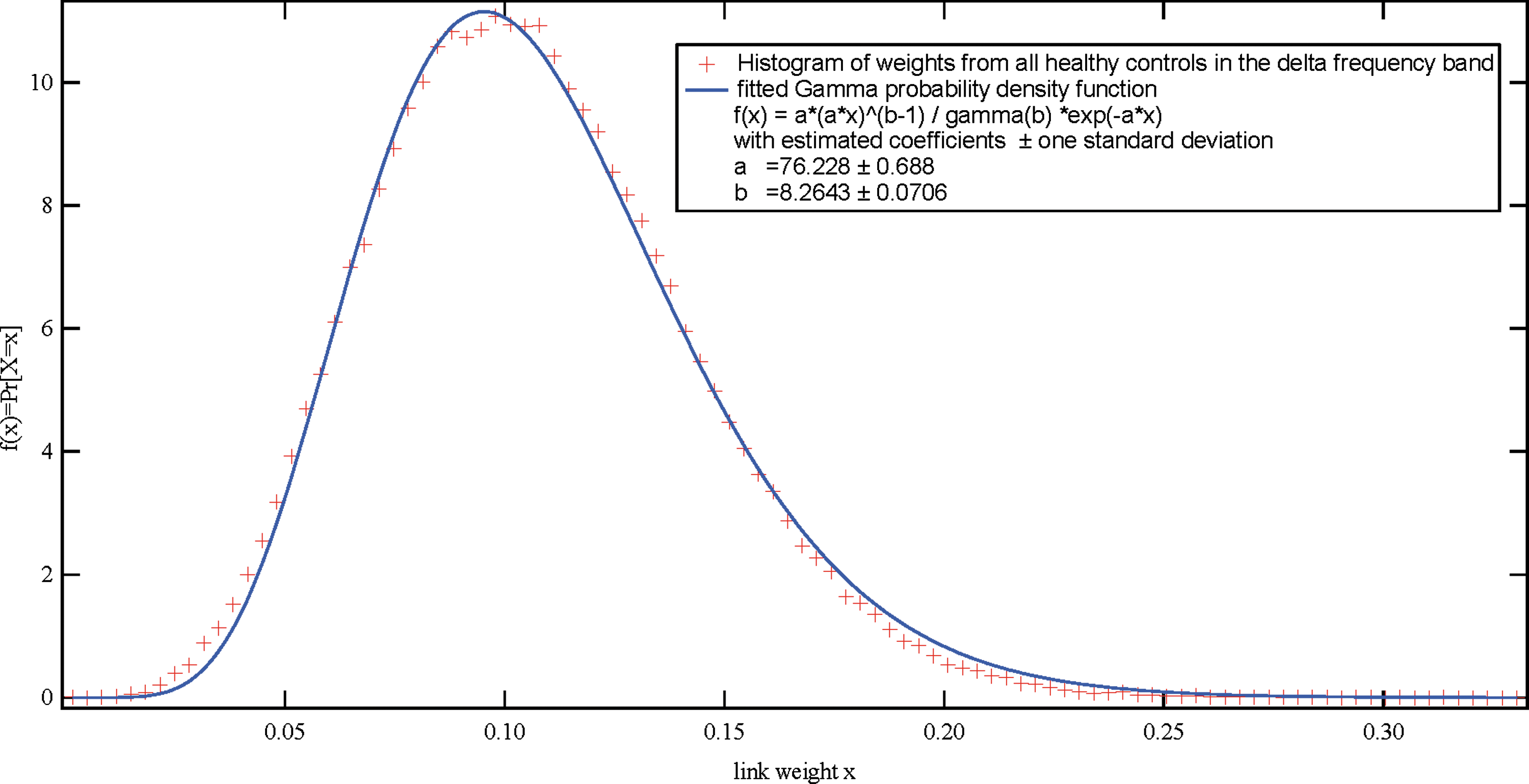
Histogram of all the link weights (after averaging over five epochs) from all PLI matrices of the delta frequency band of all 68 healthy controls. PLI, phase lag index. Color images available online at www.liebertpub.com/brain

FIG. 4.

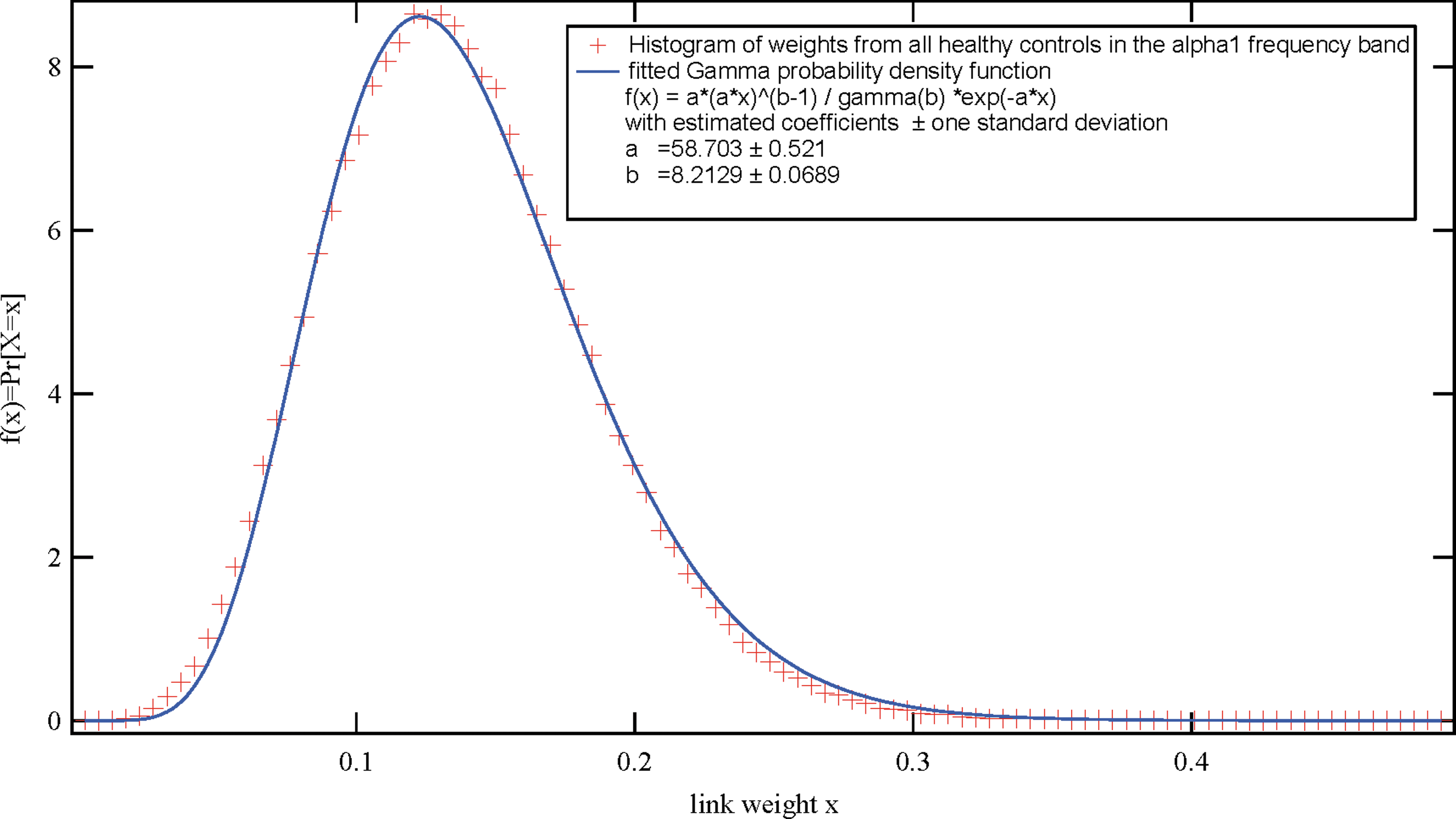
Histogram of all the link weights (after averaging over five epochs) from all PLI matrices of the alpha1 frequency band of all 68 healthy controls. Color images available online at www.liebertpub.com/brain

To sum up, we found that our USPT method picks up most of the differences found in a previous study between MS patients and controls. Overall, this previous study (Tewarie et al., 2014) found significant differences for the functional brain network between MS patients and controls in three frequency bands, delta, theta, and alpha2, with the help of conventional network analysis and testing the overall mean PLI values against each other. The performed MST analysis on the same data set seemed to only find the differences in the alpha2 band (Tewarie et al., 2014) and provides meaningful interpretation for those differences concerning the overall integration of communication that seems to be disrupted in MS patients. Our USPT method enlarges the analysis and incorporates the differences in the remaining frequency bands, the delta and theta bands. For these frequency bands, the USPT method can enhance our insight concerning the overall communication in the functional brain networks of MS patients. In another study, Goñi and associates (2014) applied the same link weight transformation, v_ij =−ln(w_ij ) to the structural brain network without giving further rationale for this specific transform. Furthermore, Goñi and associates (2014) also confirmed that the shortest path weights calculated under the link weight transformation v_ij =−ln(w_ij ) play a major role in brain network communication. Our article provided a detailed argument on why the v_ij =−ln(w_ij ) transform is a reasonable choice for the link weights of the functional brain network and showed that the topology of the resulting shortest paths can be used to differentiate between patients and healthy controls.

Conclusion

We found statistically significant differences between MS patients and controls while analyzing the link density of their USPT under the link weight transformation v_ij =−ln(w_ij ) derived from the interpretation of the link weights as independent communication probabilities. Those differences were found in the same frequency bands as in a previous study on a similar data set (Tewarie et al., 2014). As a conclusion of our findings, we propose the USPT under the link weight transformation v_ij =−ln(w_ij ) as a new sampling method for extracting differences between the functional brain networks of patients and healthy controls. The interpretation of the link weights as communication probabilities leads to a USPT of the functional brain network that includes all important links of the global brain communication.

Footnotes

Acknowledgments

This work was supported by a private sponsorship to the VUmc MS Center Amsterdam. The VUmc MS Center Amsterdam is sponsored through a program grant by the Dutch MS Research Foundation (grant number 09-358d).

Author Disclosure Statement

No competing financial interests exist.

References

Braunstein

, Wu

, Chen

, Buldyrev

, Kalisky

, Sreenivasan

, Cohen

, Lopez

, Havlin

, Stanley

. 2007. Optimal path and minimal spanning trees in random weighted networks. Int J Bifurcat Chaos, 17:2215–2255.

Bullmore

, Sporns

. 2009. Complex brain networks: graph theoretical analysis of structural and functional systems. Nat Rev Neurosci, 10:186–198.

Bullmore

, Sporns

. 2012. The economy of brain network organization. Nat Rev Neurosci, 13:336–349.

Dubbelink

KTO

, Hillebrand

, Stoffers

, Deijen

, Twisk

, Stam

, Berendse

. 2014. Disrupted brain network topology in Parkinson's disease: a longitudinal magnetoencephalography study. Brain, 137:197–207.

Gong

, He

, Concha

, Lebel

, Gross

, Evans

, Beaulieu

. 2009. Mapping anatomical connectivity patterns of human cerebral cortex using in vivo diffusion tensor imaging tractography. Cereb Cortex, 19:524–536.

Goñi

, van den Heuvel

, Avena-Koenigsberger

, de Mendizabal

, Betzel

, Griffa

, Hagmann

, Corominas-Murtra

, Thiran

J-P

, Sporns

. 2014. Resting-brain functional connectivity predicted by analytic measures of network communication. Proc Natl Acad Sci U S A, 111:833–838.

Hillebrand

, Barnes

, Bosboom

, Berendse

, Stam

. 2012. Frequency-dependent functional connectivity within resting-state networks: an atlas-based MEG beamformer solution. Neuroimage, 59:3909–3921.

Stam

, Nolte

, Daffertshofer

. 2007. Phase lag index: assessment of functional connectivity from multi-channel EEG and MEG with diminished bias from common sources. Hum Brain Mapp, 28:1178–1193.

Stam

, Tewarie

, Van Dellen

, van Straaten

, Hillebrand

, Van Mieghem

. 2014. The trees and the forest: characterization of complex brain networks with minimum spanning trees. Int J Psychophysiol, 92:129–138.

10.

Stam

, Van Straaten

. 2012. The organization of physiological brain networks. Clin Neurophysiol, 123:1067–1087.

11.

Tewarie

, Schoonheim

, Schouten

, Polman

, Balk

, Uitdehaag

, Geurts

, Hillebrand

, Barkhof

, and Stam

. 2015. Functional brain networks: linking thalamic atrophy to clinical disability in multiple sclerosis, a multimodal fMRI and MEG study. Hum Brain Mapp, 36:603–6018.

12.

Tewarie

, Steenwijk

, Tijms

, Daams

, Balk

, Stam

, Uitdehaag

, Polman

, Barkhof

, Pouwels

, Vrenken

, Hillebrand

. 2014. Disruption of structural and functional networks in long-standing multiple sclerosis. Hum Brain Mapp, 35:5946–5961.

13.

Tzourio-Mazoyer

, Landeau

, Papathanassiou

, Crivello

, Etard

, Delcroix

, Mazoyer

, Joliot

. 2002. Automated anatomical labeling of activations in SPM using a macroscopic anatomical parcellation of the MNI MRI single-subject brain. Neuroimage, 15:273–289.

14.

van Dellen

, Douw

, Hillebrand

, de Witt Hamer

, Baayen

, Heimans

, Reijneveld

, Stam

. 2014. Epilepsy surgery outcome and functional network alterations in longitudinal MEG: a minimum spanning tree analysis. Neuroimage, 86:354–363.

15.

Van Mieghem

. 2011a. Data Communications Networking. Delft, The Netherlands: Delft University of Technology.

16.

Van Mieghem

. 2011b. Graph Spectra for Complex Networks. Cambridge, United Kingdom: Cambridge University Press.

17.

Van Mieghem

. 2014. Performance Analysis of Complex Networks and Systems. Cambridge, United Kingdom: Cambridge University Press.

18.

Van Mieghem

, Magdalena

. 2005. Phase transition in the link weight structure of networks. Phys Rev E Stat Nonlin Soft Matter Phys, 72:056138.

19.

Van Mieghem

, van Langen

. 2005. Influence of the link weight structure on the shortest path. Phys Rev E Stat Nonlin Soft Matter Phys, 71:056113

20.

Van Mieghem

, Wang

. 2009. The observable part of a network. IEEE ACM Trans Network, 17:93–105.

21.

van Wijk

, Stam

, Daffertshofer

. 2010. Comparing brain networks of different size and connectivity density using graph theory. PLoS One, 5:e13701.

22.

Wang

, Douw

, Hernandez

, Reijneveld

, Stam

, Van Mieghem

. 2010. Effect of tumor resection on the characteristics of functional brain networks. Phys Rev E Stat Nonlin Soft Matter Phys, 82:021924.