Information Flow Between Resting-State Networks

Abstract

The resting brain dynamics self-organize into a finite number of correlated patterns known as resting-state networks (RSNs). It is well known that techniques such as independent component analysis can separate the brain activity at rest to provide such RSNs, but the specific pattern of interaction between RSNs is not yet fully understood. To this aim, we propose here a novel method to compute the information flow (IF) between different RSNs from resting-state magnetic resonance imaging. After hemodynamic response function blind deconvolution of all voxel signals, and under the hypothesis that RSNs define regions of interest, our method first uses principal component analysis to reduce dimensionality in each RSN to next compute IF (estimated here in terms of transfer entropy) between the different RSNs by systematically increasing k (the number of principal components used in the calculation). When k=1, this method is equivalent to computing IF using the average of all voxel activities in each RSN. For k≥1, our method calculates the k multivariate IF between the different RSNs. We find that the average IF among RSNs is dimension dependent, increasing from k=1 (i.e., the average voxel activity) up to a maximum occurring at k=5 and to finally decay to zero for k≥10. This suggests that a small number of components (close to five) is sufficient to describe the IF pattern between RSNs. Our method—addressing differences in IF between RSNs for any generic data—can be used for group comparison in health or disease. To illustrate this, we have calculated the inter-RSN IF in a data set of Alzheimer's disease (AD) to find that the most significant differences between AD and controls occurred for k=2, in addition to AD showing increased IF w.r.t. controls. The spatial localization of the k=2 component, within RSNs, allows the characterization of IF differences between AD and controls.

Introduction

The overall brain dynamics generated at rest can be decomposed as a superposition of multiple activation patterns, the so-called resting-state networks (RSNs). Being a fundamental characteristic of brain function, RSNs are a pivotal element for understanding the dynamics and organization of the brain basal activity in health and disease (Fox et al., 2005; Raichle, 2009; Raichle and Mintum, 2006; Raichle and Snyder, 2007; Raichle et al., 2001). RSNs emerge from the correlation in signal fluctuations across brain regions during the resting state, a condition defined by the absence of goal-directed behavior or salient stimuli. Despite the simplicity of the context in which these brain activity patterns are generated, RSN dynamics is rich and complex. Different RSNs have been associated with specific cognitive networks, for example, there are visual networks, sensorimotor networks, auditory networks, default mode networks (DMNs), executive control networks, and some others [for further details, see for instance Beckmann et al. (2005) and references therein].

Currently, it is well established that a number of techniques, such as region-of-interest (ROI) approach (seed-based), independent component analysis (ICA), and partial least squares, can decompose the resting-state functional magnetic resonance images (rs-fMRI) to provide such RSNs (Bell and Sejnowski, 1995; Beckmann and Smith, 2004; Beckmann et al., 2005; McIntosh and Lobaugh, 2004; Zhang and Raichle, 2010). Using these techniques, altered functional connectivity in specific RSNs has been described in brain pathological conditions, such as in patients with deficit of consciousness after traumatic brain injury (Boveroux et al., 2010; Heine et al., 2012; Maki-Marttunen et al., 2013; Noirhomme et al., 2010), schizophrenia (Karbasforoushan and Woodward, 2012; Woodward et al., 2011), and epilepsy (Liao et al., 2010). In the particular case of Alzheimer's disease (AD), the pathology we have addressed here, starting from the pioneer contribution showing alterations in fMRI (Li et al., 2002), thereon a decrease of functional connectivity in the DMN (an RSN-related memory function) and in the salience network at both early and advanced stages of the AD (Binnewijzend et al., 2012; Greicius et al., 2004; Rombouts et al., 2005; Sheline and Raichle, 2013) has been reported.

Despite this emphasis on specific networks, it is important to realize, however, that the functional division of RSN into separate systems does not imply that the brain activity comprises functional networks working in isolation (Damoiseaux et al., 2006). Contrarily, the brain regions underlying the inter-RSN relationships have their independent organization and have a different function to the specific one that each individual RSN has [for recent reviews, see Fornito et al. (2013) and Smith et al. (2013)]. These interactions between brain regions belonging to different RSNs have been described by means of whole-brain connectivity analysis techniques such as graph analysis (Bullmore and Sporns, 2009; Reijneveldand et al., 2007; Sporns et al., 2004; Stam and Reijneveld, 2007), and more recently, connectivity was also analyzed during different cognitive tasks conditions (McLaren et al., 2014).

However, the analysis and interpretation of information flow (IF) between the RSNs remain an open question and have given rise to two contrasting theories attempting to interpret the resting brain activity. The functional integration theory [for review, see Zhang and Raichle (2010)] proposes that brain activity during the resting state requires the coordinated activity of all brain RSNs to support the reconstruction, analysis, and simulation of experiences or possible scenarios to provide adaptive behavioral advantage. On the other hand, the functional segregation theory states that modality-specific mental activity (e.g., image- or language-based thoughts) is related to functional disconnection between the brain networks active during rest (Delamillieure et al., 2010). Therefore, resting activity would be maintained by functionally segregated inner-oriented and sensory-related cognition and the respective intrinsic and extrinsic brain networks they depend on.

The question of how different RSNs speak to each other is particularly relevant as it has reported the existence of disease-driven changes in functional connectivity between different brain networks (Sanz-Arigita et al., 2010; Schoonheim et al., 2013). Importantly, as the disease progresses, responsible RSNs are in turn affected, and this gradual loss of functional connectivity within networks is accompanied by a loss of functional correlation between them (Brier et al., 2012). This indicates that altered functional activity induced by a local dysfunction might influence the functioning of additional brain regions, leading to the spread of changes in brain activity beyond the network originally affected and, in turn, the whole-brain functional connectivity pattern (Sanz-Arigita et al., 2010).

In this study, we propose a new method to study RSN intercommunication. The method is based on the inference of IF in terms of transfer entropy (TE) to study directed functional connectivity (DFC) between RSNs.¹ We apply this method to AD (with the aim of showing one potential application, but the method is general and can be applied to any other disease). The first step is to consider RSNs to function as spatial templates, that is, masks, similar to the ones reported in Beckmann et al. (2005). Similar approaches, considering the RSN masks rather than the independent components per se, have been used before in previous work (Carhart-Harris et al., 2014; Haimovici et al., 2013; Tagliazucchi et al., 2012, 2014). Next, we extracted all the time series of rs-fMRI activity belonging to each RSN. After hemodynamic response function (HRF) blind deconvolution of all activity signals, our method does not work out with the average of all voxel activities per RSN, rather it approximates the global RSN activity by a k-component signal obtained by principal component analysis (PCA). The IF between regions is thus evaluated as the number of components of k is varied, while the complexity of the model is controlled by statistical testing. The standard TE analysis is recovered when (i) no HRF deconvolution is made and (ii) just the first principal component is used to describe each RSN (which is equivalent to the average over voxels within that RSN).

To show one potential application of this method, we apply it to a data set of AD patients from the Alzheimer's Disease Neuroimaging Initiative (ADNI) and compared the results of inter-RSN communication with a group of healthy subjects.

Materials and Methods

Alzheimer's Disease Neuroimaging Initiative

Data used in the preparation of this article were obtained from the ADNI database (adni.loni.ucla.edu). ADNI was launched in 2003 by the National Institute on Aging (NIA), the National Institute of Biomedical Imaging and Bioengineering (NIBIB), the Food and Drug Administration (FDA), private pharmaceutical companies, and nonprofit organizations as a $60 million, 5-year public–private partnership. The primary goal of ADNI has been to test whether serial MRI, positron emission tomography, other biological markers, and clinical and neuropsychological assessment can be combined to measure the progression of mild cognitive impairment (MCI) and early AD. Determination of sensitive and specific markers of very early AD progression is intended to aid researchers and clinicians to develop new treatments and monitor their effectiveness, as well as lessen the time and cost of clinical trials.

The principal investigator of this initiative is Michael W. Weiner, MD, VA Medical Center, University of California, San Francisco. ADNI is the result of efforts of many coinvestigators from a broad range of academic institutions and private corporations, and subjects have been recruited from over 50 sites across the United States and Canada. The initial goal of ADNI was to recruit 800 subjects, but ADNI has been followed by ADNI-GO and ADNI-2. To date, these three protocols have recruited over 1500 adults, aged 55–90, to participate in the research, consisting of cognitively normal older individuals, people with early or late MCI, and people with early AD. The follow-up duration of each group is specified in the protocols for ADNI-1, ADNI-2, and ADNI-GO. Subjects originally recruited for ADNI-1 and ADNI-GO had the option to be followed in ADNI-2. For up-to-date information, see www.adni-info.org.

Subjects

The analysis was performed on n=10 healthy subjects as control (5 males, 5 females, 73.70±1.16 years old) and n=10 AD patients (5 males, 5 females, 73.40±1.08 years old) and both data sets were downloaded from the ADNI database.

Notice that rather than increasing the population size to a very large number, we preferred to select two small populations, choosing the most balanced as possible with regard to age and gender. Demographic data (including the ADNI identifier) are given in Tables 1 and 2.

Table 1.

Alzheimer's Disease Patients

ADNI ID	Sex	Age
002 S 5018	M	73
006 S 4867	M	75
018 S 4696	F	73
018 S 5074	F	75
100 S 5106	M	74
130 S 4641	F	74
130 S 4984	F	73
130 S 5059	M	73
136 S 4993	F	72
006 S 4546	M	72

ADNI, Alzheimer's Disease Neuroimaging Initiative.

Table 2.

Healthy Subjects

ADNI ID	Sex	Age
006 S 4485	M	73
006 S 4150	M	75
002 S 4262	F	73
002 S 4270	F	75
012 S 4026	M	74
002 S 4264	F	74
018 S 4349	F	73
018 S 4400	M	72
031 S 4032	F	72
002 S 4225	M	72

MRI acquisition and preprocessing

High-resolution anatomical scans and T2-weighted rs-fMRI data were used from each subject. For the fMRI data, a total of 140 volumes were acquired with a repetition time (TR) of 3000 msec and 64×64 matrix with 48 oblique axial slices (voxel size: 3.3125×3.3125×3.3125 mm). The fMRI preprocessing was performed using FSL (FMRIB Software Library v5.0) and AFNI (Cox, 1996). Data were motion corrected and smoothened using a Gaussian Kernel of 6-mm full width at half maximum. After intensity normalization, a low-pass filter was applied within the slow fluctuations range (0.01–0.1 Hz) that characterizes the resting-state blood oxygen level-dependent (BOLD) activity. Next, linear and quadratic trends were removed. Finally, motion time courses, white matter signal, cerebrospinal fluid signal, and global signal were regressed out from the data.

ROI definition from RSN masks

We defined each ROI as the voxels belonging to each RSN by using the masks reported in Beckmann et al. (2005). These masks can be downloaded from www.fmrib.ox.ac.uk/analysis/royalsoc8/. Notice that we are not dealing with the independent components per se, but with the multivariate activity of all the voxel time series localized within the masks. Specifically, we have used the following eight RSNs: medial visual, lateral visual, auditory, sensorimotor, default mode, executive control, dorsal visual right, and dorsal visual left. fMRI data were transformed to the MNI152 template (at 3×3×3 mm resolution) and all the time series from the voxels belonging to each RSN where extracted to define each ROI. The size for each ROI is given in Table 3.

Table 3.

Resting-State Network Mask Size

RSN name	Number of voxels
Medial visual	5649
Lateral visual	8470
Auditory	10,894
Sensorimotor	7668
Default mode	8201
Executive control	15,209
Dorsal visual right	12,197
Dorsal visual left	10,524

RSN, resting-state network.

HRF blind deconvolution

We individuated point processes corresponding to signal fluctuations with a given signature and extracted a voxel-specific HRF to be used for deconvolution after following an alignment procedure. The parameters for blind deconvolution were chosen with a physiological meaning, according to Wu et al. (2013): for a TR equal to 3 sec, the threshold was fixed at 1 SD (standard deviation) and the maximum time lag varied from 3 to 5 TR, but results did not change. Results in the article have been observed for a maximum time lag equal to 5 TR. For further details on the complete HRF blind deconvolution method and the different parameters to be used, see Wu et al. (2013). The resulting time series after the HRF blind deconvolution are the ones used for the calculation of the IF.

IF between RSNs

Let us consider two RSNs, A and B. We use TE to estimate IF from A to B, and vice versa; TE is equivalent to Granger causality (GC) in the Gaussian case (Barnett et al., 2009), which is the case considered here. Let A be described by the N_A continuous time series \documentclass{aastex}\usepackage{amsbsy}\usepackage{amsfonts}\usepackage{amssymb}\usepackage{bm}\usepackage{mathrsfs}\usepackage{pifont}\usepackage{stmaryrd}\usepackage{textcomp}\usepackage{portland, xspace}\usepackage{amsmath, amsxtra}\pagestyle{empty}\DeclareMathSizes{10}{9}{7}{6}\begin{document}$$\{ { \rm x}^{ \rm A}_ \alpha ( { \rm t} ) \} _{ \alpha = 1 , \ldots , { \rm N_A}}$$ \end{document} (i.e., set of voxels belonging to region A) and B be described by the N_B continuous time series \documentclass{aastex}\usepackage{amsbsy}\usepackage{amsfonts}\usepackage{amssymb}\usepackage{bm}\usepackage{mathrsfs}\usepackage{pifont}\usepackage{stmaryrd}\usepackage{textcomp}\usepackage{portland, xspace}\usepackage{amsmath, amsxtra}\pagestyle{empty}\DeclareMathSizes{10}{9}{7}{6}\begin{document}$$\{ { \rm x}^{ \rm B}_ \alpha ( { \rm t} ) \} _{ \alpha = 1 , \ldots , { \rm N_B}}$$ \end{document} . All the time series have been deconvolved by the HRF. Fixing the number k of the principal components, the same for A and B, we represent the dynamics for A as \documentclass{aastex}\usepackage{amsbsy}\usepackage{amsfonts}\usepackage{amssymb}\usepackage{bm}\usepackage{mathrsfs}\usepackage{pifont}\usepackage{stmaryrd}\usepackage{textcomp}\usepackage{portland, xspace}\usepackage{amsmath, amsxtra}\pagestyle{empty}\DeclareMathSizes{10}{9}{7}{6}\begin{document}$$\{ { \rm y}^{{ \rm A}}_{{ \rm i}} ( { \rm t} ) \} _{{ \rm i} = 1 , \ldots , { \rm k}}$$ \end{document} and for B as \documentclass{aastex}\usepackage{amsbsy}\usepackage{amsfonts}\usepackage{amssymb}\usepackage{bm}\usepackage{mathrsfs}\usepackage{pifont}\usepackage{stmaryrd}\usepackage{textcomp}\usepackage{portland, xspace}\usepackage{amsmath, amsxtra}\pagestyle{empty}\DeclareMathSizes{10}{9}{7}{6}\begin{document}$$\{ { \rm y}^{{ \rm B}}_{{ \rm i}} ( { \rm t} ) \} _{{ \rm i} = 1 , \ldots , { \rm k}}$$ \end{document} . Note that these components are statistically independent in the Gaussian approximation. Given the order m (the number of past points to be included in the state vector) and the lag parameter δ, we denote the ith component of the state vector as follows: \documentclass{aastex}\usepackage{amsbsy}\usepackage{amsfonts}\usepackage{amssymb}\usepackage{bm}\usepackage{mathrsfs}\usepackage{pifont}\usepackage{stmaryrd}\usepackage{textcomp}\usepackage{portland, xspace}\usepackage{amsmath, amsxtra}\pagestyle{empty}\DeclareMathSizes{10}{9}{7}{6}\begin{document} \begin{align*}Y^A_i ( t ) = \left( y^A_i ( t - \delta ) \cdots y^A_i ( t - \delta - m ) \right) , \tag{1}\end{align*} \end{document}

and the corresponding one for B as follows: \documentclass{aastex}\usepackage{amsbsy}\usepackage{amsfonts}\usepackage{amssymb}\usepackage{bm}\usepackage{mathrsfs}\usepackage{pifont}\usepackage{stmaryrd}\usepackage{textcomp}\usepackage{portland, xspace}\usepackage{amsmath, amsxtra}\pagestyle{empty}\DeclareMathSizes{10}{9}{7}{6}\begin{document} \begin{align*}Y^B_i ( t ) = \left( y^B_i ( t - \delta ) \cdots y^B_i ( t - \delta - m ) \right). \tag{2}\end{align*} \end{document}

According to the Akaike information criterion, we use m=1. The calculation of IF from A to B depends on the used lag δ. In this study, in addition to lag equal to 1, we also simulated δ=2 (corresponding to 6 sec as TR=3 sec) and δ=3 (9 sec), showing slightly different behavior. In particular, for both δ=2 and δ=3, we still found an increase of IF in AD w.r.t. controls, but that increment was not significant in any number of principal components (k). Thus, only for δ=1, the case we have considered here, the increment of IF occurring in AD was statistically significant (for both k=2 and k=3).

To evaluate the IF from A to B, we first calculate the IF from A to the ith component of B, that is, \documentclass{aastex}\usepackage{amsbsy}\usepackage{amsfonts}\usepackage{amssymb}\usepackage{bm}\usepackage{mathrsfs}\usepackage{pifont}\usepackage{stmaryrd}\usepackage{textcomp}\usepackage{portland, xspace}\usepackage{amsmath, amsxtra}\pagestyle{empty}\DeclareMathSizes{10}{9}{7}{6}\begin{document} \begin{align*} \begin{split} t \left( A \rightarrow B^i \right) = H ( y^B_i \mid \{ Y^B_j \} _{j = 1 , \ldots , k} ) \\- H ( y^B_i \mid \{ Y^B_j \} _{j = 1 , \ldots , k}; \{ Y^A_j \} _{j = 1 , \ldots , k} ),\end{split} \tag{3}\end{align*} \end{document}

where H is the conditional Shannon entropy, evaluated over the empirical distribution of samples at hand under the assumption of Gaussianity, see Barnett et al. (2009). Notice two important issues from Equation (3): first, that the two conditioned states, \documentclass{aastex}\usepackage{amsbsy}\usepackage{amsfonts}\usepackage{amssymb}\usepackage{bm}\usepackage{mathrsfs}\usepackage{pifont}\usepackage{stmaryrd}\usepackage{textcomp}\usepackage{portland, xspace}\usepackage{amsmath, amsxtra}\pagestyle{empty}\DeclareMathSizes{10}{9}{7}{6}\begin{document}$$\{ Y^B_j \} _{j = 1 , \ldots , k}$$ \end{document} and \documentclass{aastex}\usepackage{amsbsy}\usepackage{amsfonts}\usepackage{amssymb}\usepackage{bm}\usepackage{mathrsfs}\usepackage{pifont}\usepackage{stmaryrd}\usepackage{textcomp}\usepackage{portland, xspace}\usepackage{amsmath, amsxtra}\pagestyle{empty}\DeclareMathSizes{10}{9}{7}{6}\begin{document}$$\{ Y^A_j \} _{j = 1 , \ldots , k}$$ \end{document} , are accounting for lagged interactions, that is, the two depend on the δ parameter appearing in Equations (1) and (2), but the term \documentclass{aastex}\usepackage{amsbsy}\usepackage{amsfonts}\usepackage{amssymb}\usepackage{bm}\usepackage{mathrsfs}\usepackage{pifont}\usepackage{stmaryrd}\usepackage{textcomp}\usepackage{portland, xspace}\usepackage{amsmath, amsxtra}\pagestyle{empty}\DeclareMathSizes{10}{9}{7}{6}\begin{document}$$y^B_i$$ \end{document} is not lagged. Second, that the interaction given by Equation (3) is univariate for the target and multivariate for the driver.

Next, repeating the same as in Equation (3) for each of the components in B, that is, i=1,…,k, and denoting π_i as the probability of \documentclass{aastex}\usepackage{amsbsy}\usepackage{amsfonts}\usepackage{amssymb}\usepackage{bm}\usepackage{mathrsfs}\usepackage{pifont}\usepackage{stmaryrd}\usepackage{textcomp}\usepackage{portland, xspace}\usepackage{amsmath, amsxtra}\pagestyle{empty}\DeclareMathSizes{10}{9}{7}{6}\begin{document}$${ \rm t} ( { \rm A} \rightarrow { \rm B}^{ \rm i} )$$ \end{document} under the null hypothesis of the absence of influence, both π_i and \documentclass{aastex}\usepackage{amsbsy}\usepackage{amsfonts}\usepackage{amssymb}\usepackage{bm}\usepackage{mathrsfs}\usepackage{pifont}\usepackage{stmaryrd}\usepackage{textcomp}\usepackage{portland, xspace}\usepackage{amsmath, amsxtra}\pagestyle{empty}\DeclareMathSizes{10}{9}{7}{6}\begin{document}$${ \rm t} ( { \rm A} \rightarrow { \rm B}^{ \rm i} )$$ \end{document} can be calculated analytically in the Gaussian approximation, cf, in Equation (12) in the article (Barnett et al., 2009). Finally, IF is then estimated as the average over all components in B, that is, \documentclass{aastex}\usepackage{amsbsy}\usepackage{amsfonts}\usepackage{amssymb}\usepackage{bm}\usepackage{mathrsfs}\usepackage{pifont}\usepackage{stmaryrd}\usepackage{textcomp}\usepackage{portland, xspace}\usepackage{amsmath, amsxtra}\pagestyle{empty}\DeclareMathSizes{10}{9}{7}{6}\begin{document} \begin{align*}IF ( A \rightarrow B ) = \frac { 1 } { k } \sum \nolimits^k_ { i = 1 } \theta \left( \frac { \tau } { k } - \pi_i \right) t ( A \rightarrow B^i ) , \tag { 4 } \end{align*} \end{document}

where θ is the Heaviside function that makes the sum to account for all the contributions, which are statistically significant according to Bonferroni criterion, that is, those with π_i<τ/k, where τ is the statistical significance (we use 0.05 here).

The complexity of the model is thus controlled by statistical testing, that is, accepting only significant interactions [a similar strategy to control complexity is used in Marinazzo et al. (2008)].

Statistical testing

To perform statistical significance between groups in Figures 2 –4, a nonparametric Wilcoxon rank-sum test was used to validate the hypothesis that two data distributions have equal medians. This was implemented in Matlab, The MathWorks, Inc., with the function, ranksum, at p=0.05 with Bonferroni correction.

For Figure 5, a nonparametric, two-sample unpaired t-test was performed as implemented in FSL. First, the k=2 component was regressed into 4D fMRI data of each particular subject to obtain a subject-specific spatial map. Next, to search for the group differences (control vs. AD) in the spatial maps, we performed a permutation-based nonparametric inference as implemented in the function randomize in FSL, option threshold-free cluster enhancement with familywise error-corrected p=0.05.

Anatomical localization in brain differences: control versus AD

To localize the spatial maps plotted in Figure 5, we overlapped these maps with the automated anatomical labeling (AAL) atlas (Tzourio-Mazoyer et al., 2002) to get the anatomical regions underlying such differences. In particular, we calculated the overlapping percentage between all voxels in each spatial map and each of the 45 homologue brain areas existing in the AAL parcellation. Although the RSNs are widespread across the whole brain, our localization criteria only considered the percentage of voxels in each spatial map to be bigger than 15% (with respect to the total spatial map size), results are given in Table 4.

Table 4.

Localization of Brain Differences in Alzheimer's Disease Versus Control Using the Automated Anatomical Labeling Parcellation

RSN	Regions in AD, but not in control (red in Fig. 5)	Regions in control, but not in AD (blue in Fig. 5)
Medial visual	Calcarine sulcus, cuneus, lingual gyrus	Paracentral lobule
Lateral visual	Middle occipital gyrus	Superior occipital gyrus, middle occipital gyrus
Auditory	Thalamus	Superior temporal gyrus
Sensorimotor	Rolandic operculum, Heschl's gyrus, superior temporal gyrus	Precentral
Default mode	Medial frontal gyrus, thalamus	Midcingulate area, cuneus, angular gyrus
Executive control	Supramarginal gyrus	Superior frontal gyrus, middle frontal gyrus
Dorsal visual right	Inferior parietal lobule, angular gyrus	Inferior frontal gyrus pars triangularis, insula
Dorsal visual left	Angular gyrus	None upper 15% overlapping

AD, Alzheimer's disease.

Results

After extracting all voxels belonging to each RSN and deconvolving each of the individual voxels with HRF (see the Materials and Methods section), we first applied PCA to each RSN and then computed the multivariate IF between RSNs (see Fig. 1 for a chart flow). Regarding the amount of variability captured by the principal components, after averaging between subjects, about 60% of total variability was captured by the first 10 components (k=10) (Supplementary Fig. 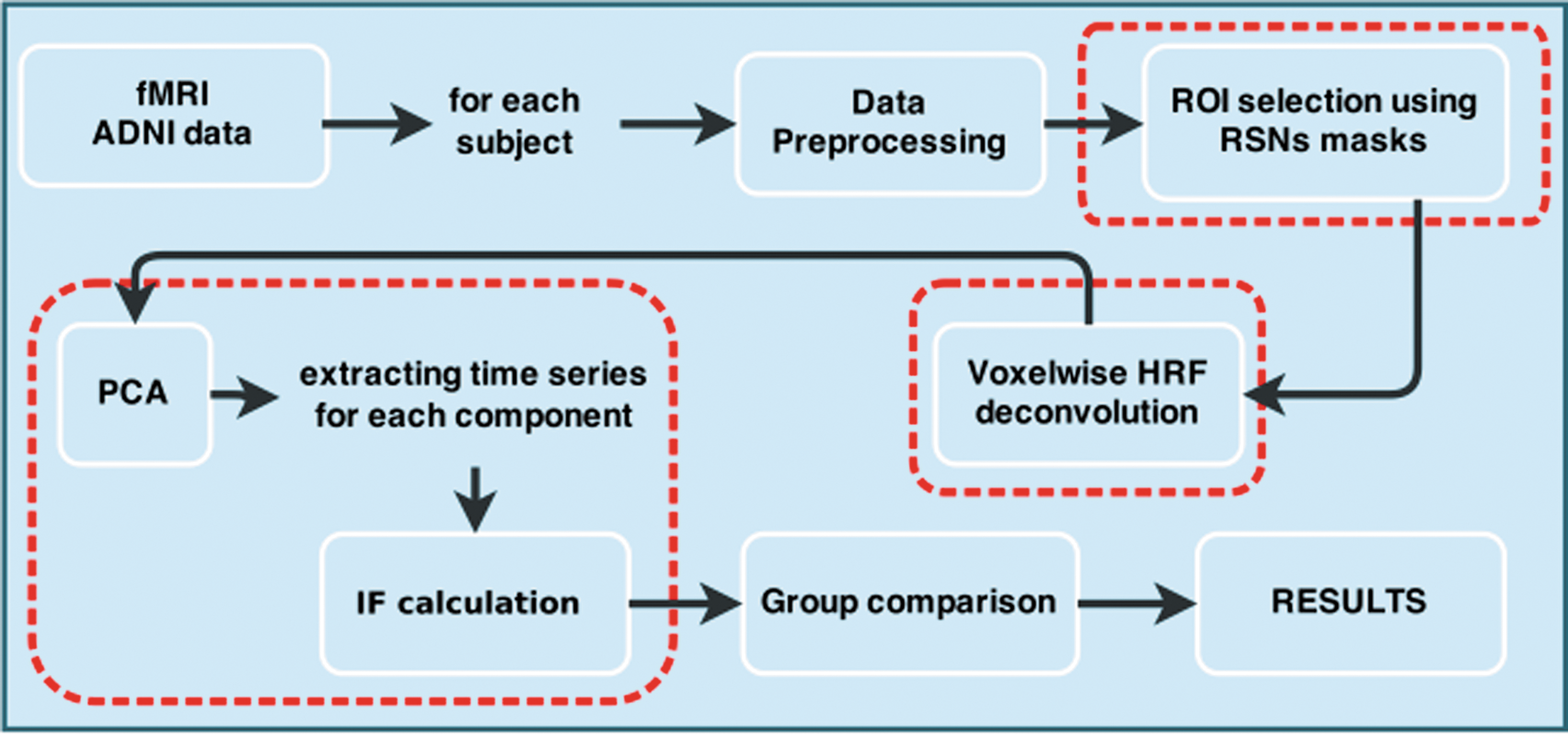S1; Supplementary Data are available online at www.liebertpub.com/brain) and 99% of total variability was captured for k=72 (Supplementary Fig. S2). No statistically significant differences were found in the amount of variability between control and AD, indicating that the data representation in the different principal components was disease independent. Therefore, the reader should not be confused and be aware that differences in IF are not related to these percentages.

FIG. 1.

Methodological sketch. Red (dashed) rectangles indicate key stages in our approach. Color images available online at www.liebertpub.com/brain

The average IF between the different RSNs is represented in Figure 2. Systematically, we recomputed IF with a different number of principal components (maintaining the same for all RSNs) from k=1 up to k=15. The case k=1 is equivalent to calculating IF between the average voxel activities for each RSN. The case k>1 corresponds to a multivariate situation. For visualization purposes, Figure 2 shows results up to k=11, and as for k≥10, the information was zero. Notice that having a zero IF is possible because, according to Equation (4), the quantity of IF is averaged over all the components. Thus, if adding a new component does not provide new independent information, the term (1/k) in the denominator will eventually decrease the average IF. To represent Figure 2, notice that as we were dealing with n=10 healthy subjects and n=10 AD patients, we first obtained for each subject a matrix of IFs, in which the element (i, j) indicated IF from the ith RSN to the jth one. Next, we pooled together all the matrices belonging to the same group (control and AD) and represented the average IF among all possible pairs—for eight RSNs, the total number of pairs is 8×(8−1)=56, which is equal to the number of pairs minus the elements in the principal diagonal. The profile of average information as a function of the number of principal components (used for calculation of the IF) is the same for control and AD: starting to increase from k=1 up to the maximum at k=5, and then begin to decrease monotonically. Therefore, we conclude that for dimensions bigger than k=5, a higher dimension does not provide more IF. Statistically significant differences for the average IF between control and AD occurred for k=2 and k=3. Interestingly, the average inter-RSN IF is higher in AD than in controls.

FIG. 2.

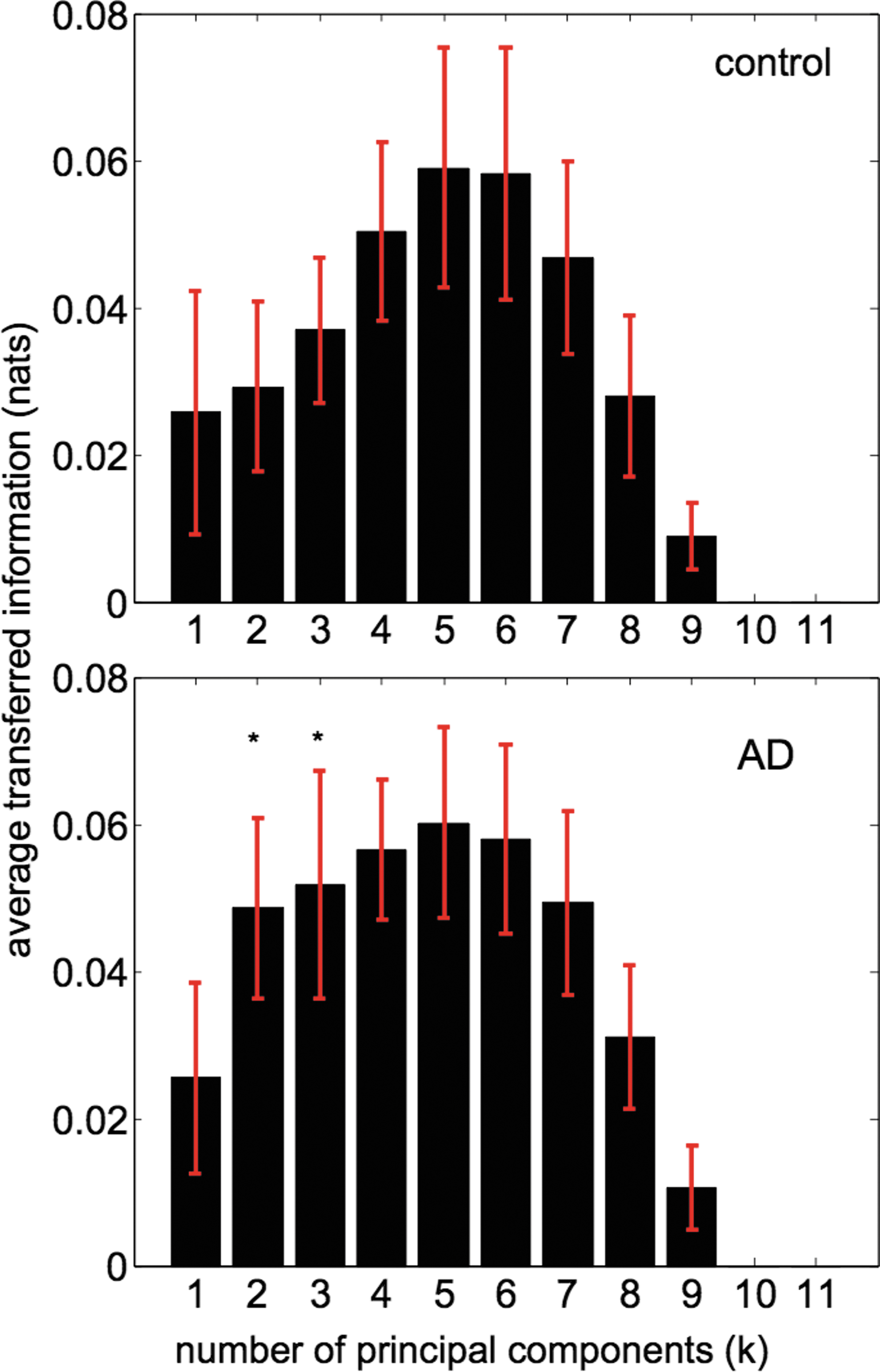
Average transferred information between all resting-state networks (RSNs) as a function of the number of principal components. Control (top) versus Alzheimer's disease (AD; bottom). The pattern of transferred information is the same for the two conditions; it increases from k=1 up to the maximum at k=5 to start to decrease up to zero information for k≥10. This means that the k=5 multivariate information flow (IF) between the different RSNs is most informative than in any other dimension. * Represents statistical differences between control and AD, p=0.05 (Bonferroni correction). Standard error (depicted in red) has been calculated across subjects for each group, control (n=10) versus AD (n=10). Information has been calculated in nats (i.e., Shannon entropies have been calculated in natural logarithms); however, to transform to information bits, we have to multiply the value in nats by 1.44. Color images available online at www.liebertpub.com/brain

Figure 3 shows all possible values of IF between all RSNs. In this study, the number of principal components was fixed to k=2 (the one with biggest statistical difference in Fig. 2), but similar graphs were obtained for each value of k. Unlike correlations, TE measures DFC, thus Figure 3 represents, for each condition control and AD, the two directions in IF (i.e., for two generic RSNs, A and B, if in the top panel we represented IF from A to B, then in the bottom panel, we depicted IF from B to A). In other words, the average value among all the flows in Figure 3 is the one plotted in Figure 2. It is important to remark that all RSNs are communicating with each other, and, as shown Figure 2, on average, the AD condition had higher information flowing between RSNs in comparison with control.

FIG. 3.

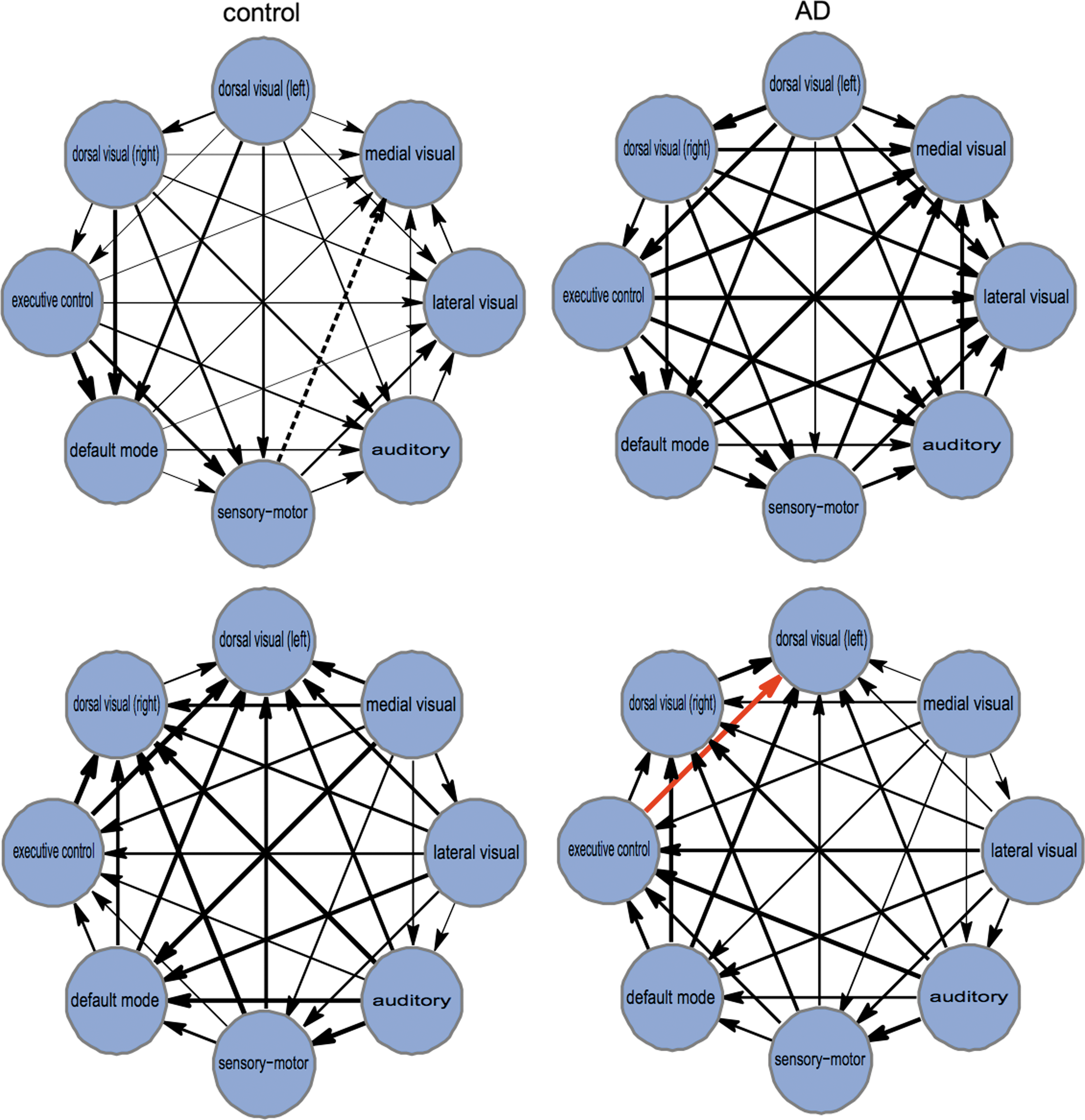
Networks of IF between the different RSNs. For k=2 (occurring as the biggest difference between control and AD in Fig. 2), we have represented the multivariate IF between the different RSNs. Control (left) versus AD (right) for the two directions of IF (top and bottom). IF values are proportional to arrow thickness. Values represented in Figure 2 are the average among all the arrows represented in this figure, taking into account the two flow directions (top and bottom). Only for visualization purposes, values of IF have been normalized to the common maximum (marked with the red arrow), corresponding to transfer entropy (TE)=0.078 nats from the executive control network to the medial visual (left) in the AD condition. Dashed arrow from the sensorimotor network to the medial visual corresponds to the minimum value, which before normalization was TE=0.006 and after normalization was fixed to zero. Color images available online at www.liebertpub.com/brain

Next, we addressed IF arriving to and originating from each specific RSN. Figure 4 shows the outward information in blue and the inward information in red. The negativity in all the bars (obtained by subtracting the information in control minus the corresponding one in AD) confirmed that within all RSNs there existed an increase of the information for AD in both the outward and the inward directions.

FIG. 4.

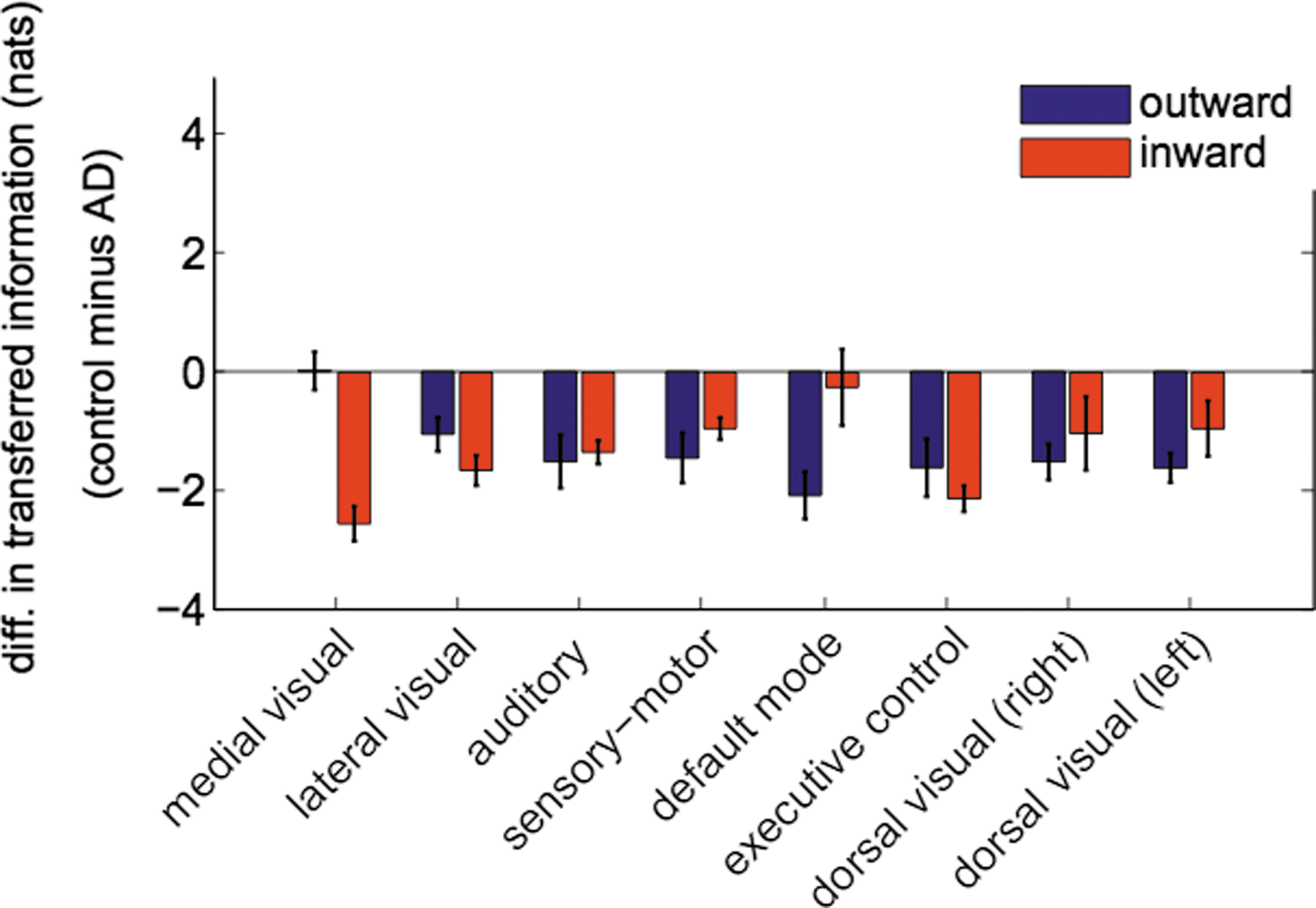
Control minus AD differences in the total IF per RSN. Outward information (blue) and inward information (red) from/to each different RSN. Error bars have been calculated across subjects for each group. Notice that values in this figure are much higher than those in Figure 2 due to two reasons: first, values in Figure 2 correspond to the average value of IF, taking off principal diagonal elements, this implied dividing each IF value by a factor of 56. Second, because to calculate both outward and inward information, we sum over columns and rows, respectively, and this meant multiplying each IF value by a factor of 6 (not including the self-node information and the element in the principal diagonal). Thus, values in this figure might be even up to 336 times bigger. Color images available online at www.liebertpub.com/brain

Finally, we performed a two-sample unpaired t-test to localize the differences between AD and control for the k=2 component. Results are shown in Figure 5; the differences are plotted in two colors: blue for the activity existing in control, but nonexistent in AD, and in red, vice versa, activated areas belonging to AD, but not to control. Next, we overlapped these maps with the AAL atlas (details in the Materials and Methods section) to get the relevant anatomical regions for each RSN, cf, in Table 4.

FIG. 5.

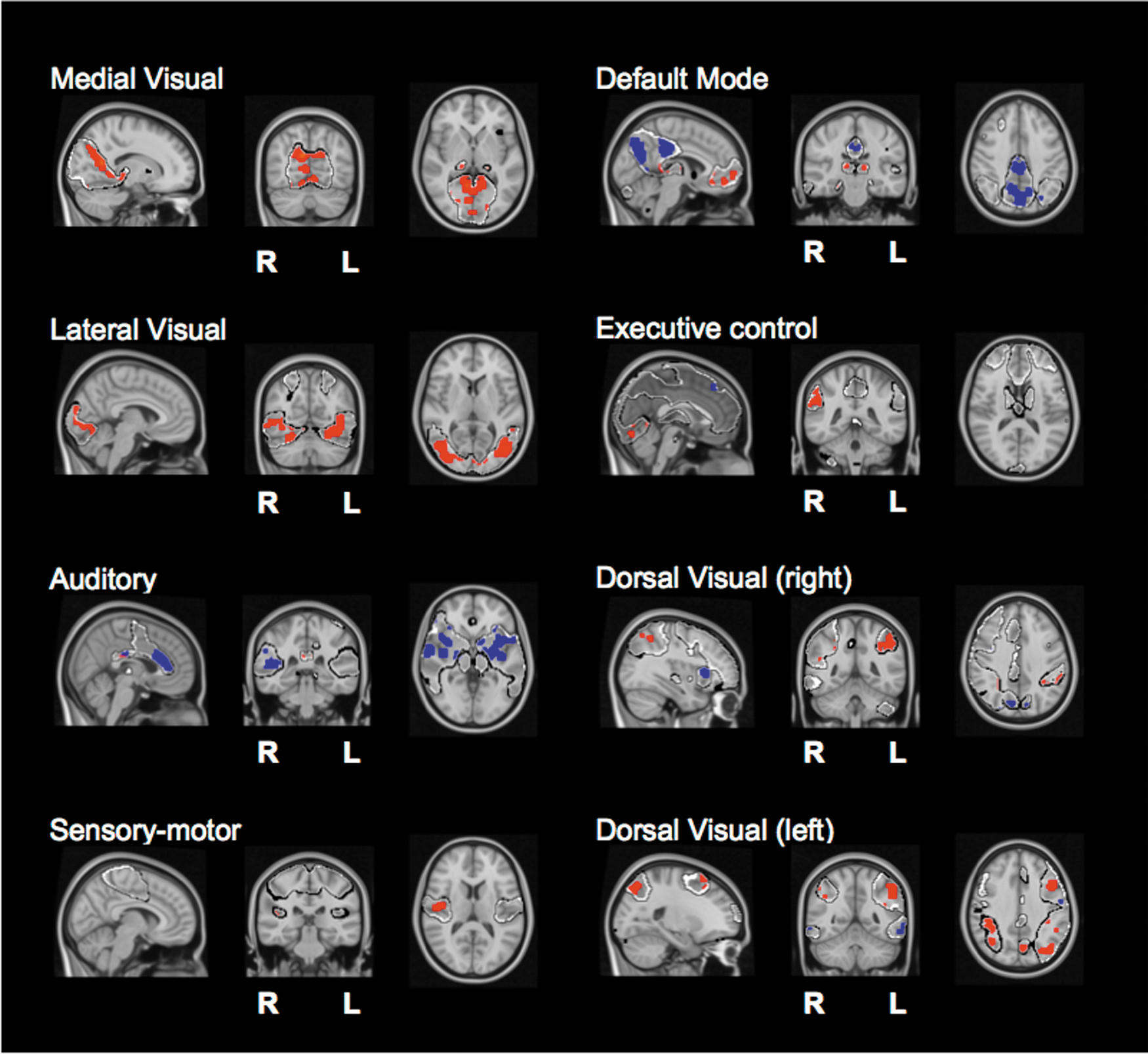
Brain maps of statistical significance localizing the k=2 component within each RSN. After a two-sample unpaired t-test (see the Materials and Methods section), we are representing two possible contrasts: in red, the figure shows the significant activity existing in AD, but nonexistent in control. In blue, vice versa, differences, which exist in control, but not in AD. Color images available online at www.liebertpub.com/brain

Discussion

RSNs are chiefly characterized by their universal emergence, meaning that beyond individual subject differences, RSNs are ubiquitous in healthy brains. While the emergence of RSNs in health is a well-known fact, how these RSNs speak to each other is not fully understood yet. In our approach, instead of applying ICA to each subject separately to get their specific RSNs, we used templates provided in Beckmann et al. (2005) for all subjects. The use of the same templates for all the subjects is indeed assuming that the spatial structure of all RSNs is universal. Our main hypothesis here is that the breakdown of this assumption might differentiate healthy subjects and AD patients—but the same method can be applied to any other disease—and that searching for such differences might provide further insights about the alteration patterns of IF in the pathological brain. In other words, we were interested in providing an answer to the following question: what are the different features in healthy versus pathological brains under the hypothesis that the same templates characterize RSNs? To this end, we introduced a novel method that calculates IF between all the different RSNs.

We applied this methodology to AD data sets and compared these results with controls. The interesting answer is that such an assumption led—for the particular situation of AD—to differences in the information related to the second and third principal components and not to the first one (which is coincident with the average activity over all voxels per RSN). Notice that from Equations (3) and (4), one can see that the TE is calculated univariately for the target and multivariately for the driver. Thus, when we say that AD versus control differences are associated with k=2, we mean a multivariate driver taking into account the two time series, k=1 and k=2. Therefore, as far as the average time series of each ROI is concerned, no differences between the patterns of healthy and AD patients emerged. Performing a paired t-test to spatially localize the k=2 component, we found the regions that were underlying those differences.

An important limitation of ROI analysis in MRI data is the huge number of voxels determining each brain region. In most cases, the average time series (across voxels at each time point) or the first principal component is assumed to be the ROI representative (we verified that the average and the first principal components are equivalent in our data set); the connectivity analyses are then carried out using these regional representative signals. However, neither the average nor the first PCA is taking into account the predictive power of past value. Thus, relevant temporal information may be diluted when considering these signals.

Some approaches have represented each ROI using more than one time series, either by using PCA (Zhou et al., 2009) or cluster analysis (Sato et al., 2010). The approach we are presenting here is rooted on principal component analysis and its novelty is based on two points: first, we preprocessed the time series corresponding to each individual voxel by HRF blind deconvolution, and second, instead of fixing the number of components according to a prescribed fraction of the data variance, as it is usually done, we have analyzed IF as the number of component increases, including more details of the ROI dynamics.

Using the RSN spatial templates (masks) reported in Beckmann et al. (2005), we extracted different ROIs to approximate each RSN by a fixed multivariate dimension (k) found by PCA. Notice that the common approach of taking the average over all voxel activities belonging to each RSN corresponds to k=1. Beyond this, the average interactions are captured by k≥1. Therefore, our method can be considered as a generalization for the average activity approach.

Recently, the point process analysis described in Tagliazucchi et al. (2012) showed that the relevant information in resting-state fMRI can be obtained by looking into discrete events resulting in relatively large amplitude BOLD signal peaks. Following this idea, we have considered the preprocessed resting fMRI time series to be spontaneous, event related, and individuated point processes corresponding to signal fluctuations with a given signature, extracting a voxel-specific HRF to be used for deconvolution.

We want to remark that the use of the HRF deconvolution, apart from being conceptually mandatory in our opinion, is also crucial for our results. Indeed, we repeated our analysis while omitting the deconvolution stage and found a clear different pattern of IF between RSNs. In particular, IF differences were only significant for k=1 and AD showed a decreased IF w.r.t. healthy subjects (Supplementary Fig. S3). We also verified that in general, the use of HRF deconvolution increased the IF for all subjects in comparison with no deconvolution. Thus, if we had omitted the HRF deconvolution stage, we would have not observed the relevant role of the second and the third principal components in shaping the differences of IF in AD and controls.

Previous work has addressed DFC between the different RSNs; for instance, the authors in Demirci et al. (2009) ICA extracted the time courses of spatially independent components and found differences in DFC between schizophrenia and control conditions. It is worth mentioning that a method for effective connectivity inference, combining PCA and GC, was proposed in Zhou et al. (2009). The main differences between our method (tailored to analyze the IF between RSNs) and the one developed in Zhou et al. (2009) are the blind deconvolution with HRF and the fact that we use the number of components as a parameter to be systematically increased (up to finding statistically significant different causalities) and both driver and target ROIs are described with the same number of components. In Zhou et al. (2009), instead, all voxels in the activated brain regions were taken as the target and the PCA analysis was applied only to the driver region and not to the target one.

Following previous work extending the use of DFC to the multivariate situation (Barnett et al., 2009; Barrett et al., 2010; Deshpande et al., 2009; Liao et al., 2011), we have applied here a multivariate DFC approach to the study of the interaction between RSNs. Specifically to AD, causal interactions among the different RSNs were addressed in Liu et al. (2012) by a multivariate GC. The authors found an increase in IF between RSNs in relation to the DMN and the executive control one, which is in agreement with the increase of IF reported here, possibly suggesting compensatory processes in the brain networks underlying AD. Similarly and more recently, an increase of connectivity in the DMN was found by other authors in Liang et al. (2014) in amnesic MCI by using GC.

The main result of the present study is the finding that the AD condition had higher IF between RSNs in comparison with control. This is apparently in contradiction to a recent article (Li et al., 2013) where a Bayesian network approach reported a general decrease in connectivity strength for AD. Moreover, the authors in Li et al. (2013) found an increase in connectivity between the DMN and the dorsal attention network when using the average voxel activity, and in our approach, this situation is equivalent to considering k=1. In this study, if we apply the HRF deconvolution preprocessing, we find no significant differences between controls and AD at k=1, but if no deconvolution is applied, k=1 for AD shows a significantly decreased IF w.r.t. healthy subjects, in full agreement with (Li et al., 2013). Moreover, for k=1, we find an increase of the interaction from the DMN to the dorsal visual (left) network and this is also consistent with the findings in Li et al. (2013). It follows that the results in the article (Li et al., 2013) are consistent with the application of our method when just one component is considered and the HRF deconvolution is omitted. Our findings suggest that in AD, the second (and, to a lesser extent, the third) components of the signals within RSNs are responsible for the increased IF. Approximating each RSN by a single signal is not enough to put in evidence these phenomena.

The IF increase found in AD might have different causes, perhaps due to a compensatory reorganization of brain circuits due to synaptic plasticity (Adams, 1991) or due to the fact that AD patients might fail in ignoring irrelevant inputs when integrating information to perform particular cognitive tasks (Rodriguez et al., 1999) or due to the reduction in inhibitory modulatory influence across the whole-brain network in AD (Amieva et al., 2004; Bentley et al., 2008; Rytsar et al., 2011); however, the exact mechanism producing an increase of IF in AD needs further investigation.

The small population size included in this study only allows for a limited interpretation of the details of connectivity changes between networks. However, a conservative approach to this analysis indicates that the IF implicated in sensory processing networks and the DMN is relatively increased in AD compared with controls. Both reductions as well as increments in functional connectivity have been previously reported between brain regions in early AD. Interestingly, most of the regional connectivity increments have been described in the frontal regions, overlapping with regions belonging to the executive control network, DMN, and frontal regions of the dorsal visual processing stream (Sanz-Arigita et al., 2010).

Footnotes

Acknowledgments

The authors acknowledge Prof. Dante R. Chialvo, who first motivated them to study information flow between RSNs, and financial support from Ikerbasque: The Basque Foundation for Science, Gobierno Vasco (Saiotek SAIO13-PE13BF001), Junta de Andalucia (P09-FQM-4682), and Euskampus at UPV/EHU to J.M.C.; Ikerbasque Visiting Professor at Biocruces and project BRAhMS–Brain Aura Mathematical Simulation (AYD-000-285), cofunded by Bizkaia Talent and European Commission through the COFUND programme to S.S.; and the predoctoral contract from the Basque Government, Eusko Jaurlaritza, grant PRE_2014_1_252, to A.E. Data collection and sharing for this project were funded by the Alzheimer's Disease Neuroimaging Initiative (ADNI) National Institutes of Health grant, U01 AG024904. ADNI is funded by the National Institute on Aging, the National Institute of Biomedical Imaging and Bioengineering, and through generous contributions from the following: Abbott, AstraZeneca AB, Amorfix, Bayer Schering Pharma AG, BioClinica, Inc., Biogen Idec, Bristol-Myers Squibb, Eisai Global Clinical Development, Elan Corporation, Genentech, GE Healthcare, Innogenetics, IXICO, Janssen Alzheimer Immunotherapy, Johnson and Johnson, Eli Lilly and Co., Medpace, Inc., Merck and Co., Inc., Meso Scale Diagnostic, LLC, Novartis AG, Pfizer, Inc., F. Hoffman-La Roche, Servier, Synarc, Inc., and Takeda Pharmaceuticals, as well as nonprofit partners, the Alzheimer's Association and Alzheimer's Drug Discovery Foundation, with participation from the U.S. Food and Drug Administration. Private sector contributions to ADNI are facilitated by the Foundation for the National Institutes of Health (www.fnih.org). The grantee organization is the Northern California Institute for Research and Education, and the study is coordinated by the Alzheimer's Disease Cooperative Study at the University of California, San Diego. ADNI data are disseminated by the Laboratory for Neuroimaging at the University of California, Los Angeles. This research was also supported by NIH grants, P30 AG010129 and K01 AG030514, and the Dana Foundation.

Author Disclosure Statement

No competing financial interests exist.

References

Adams

. 1991. Structural plasticity of synapses in Alzheimer's disease. Mol Neurobiol, 5:411–419.

Amieva

, Phillips

, Della Sala

, Henry

. 2004. Inhibitory functioning in Alzheimer's disease. Brain, 127:949–964.

Barnett

, Barrett

, Seth

. 2009. Granger causality and transfer entropy are equivalent for Gaussian variables. Phys Rev Lett, 103:238701.

Barrett

, Barnett

, Seth

. 2010. Multivariate Granger causality and generalized variance. Phys Rev E, 81:041907.

Beckmann

, DeLuca

, Devlin

, Smith

. 2005. Investigations into resting-state connectivity using independent component analysis. Philos Trans R Soc Lond B Biol Sci, 360:1001–1013.

Beckmann

, Smith

. 2004. Probabilistic independent component analysis for functional magnetic resonance imaging. IEEE Trans Med Imaging, 23:137–152.

Bell

, Sejnowski

. 1995. An information-maximization approach to blind separation and blind deconvolution. Neural Comput, 7:1129–1159.

Bentley

, Driver

, Dolan

. 2008. Cholinesterase inhibition modulates visual and attentional brain responses in Alzheimer's disease and health. Brain, 131:409–424.

Binnewijzend

, Schoonheim

, Sanz-Arigita

, Wink

, van der Flier

, Tolboom

, Adriaanseand

, Damoiseaux

, Scheltensand

, van Berckel

, Barkhof

. 2012. Resting-state fMRI changes in Alzheimer's disease and mild cognitive impairment. Neurobiol Aging, 33:2018–2028.

10.

Boveroux

, Vanhaudenhuyse

, Brun

, Noirhomme

, Lauwick

, Luxen

, Degueldre

, Plenevau

, Schnakers

, Phillips

, Brichant

, Bonhomme

, Maquet

, Greicius

, Laureys

, Boly

. 2010. Breakdown of within- and between-network resting state functional magnetic resonance imaging connectivity. Anesthesiology, 113:1038–1053.

11.

Bressler

, Seth

. 2011. Wiener-granger causality: a well-established methodology. Neuroimage, 58:323–329.

12.

Brier

, Thomasand

, Snyder

, Benzinger

, Zhang

, Raichle

, Holtzman

, Morris

, Ances

. 2012. Loss of intranetwork and internetwork resting state functional connections with Alzheimer's disease progression. J Neurosci, 32:8890–8898.

13.

Bullmore

, Sporns

. 2009. Complex brain networks: graph theoretical analysis of structural and functional systems. Nat Rev Neurosci, 10:186–198.

14.

Carhart-Harris

, Leech

, Hellyer

, Shanahan

, Feilding

, Tagliazucchi

, Chialvo

, Nutt

. 2014. The entropic brain: A theory of conscious states informed by neuroimaging research with psychedelic drugs. Front Hum Neurosci, 8:20.

15.

Cox

. 1996. AFNI: software for analysis and visualization of functional magnetic resonance neuroimages. Comput Biomed Res, 29:162–173.

16.

Damoiseaux

, Rombouts

, Barkhof

, Scheltens

, Stam

, Smith

, Beckmann

. 2006. Consistent resting-state networks across healthy subjects. Proc Natl Acad Sci U S A, 103:13848.

17.

Delamillieure

, Doucet

, Mazoyer

, Turbelin

M-R

, Delcroix

, Mellet

, Zago

, Crivello

, Petit

, Tzourio-Mazoyer

, Joliot

. 2010. The resting state questionnaire: An introspective questionnaire for evaluation of inner experience during the conscious resting state. Brain Res Bull, 81:565–573.

18.

Demirci

, Stevens

, Andreasen

, Michael

, Liu

, White

, Pearlson

, Clark

, Calhoun

. 2009. Investigation of relationships between fMRI brain networks in the spectral domain using ICA and Granger causality reveals distinct differences between schizophrenia patients and healthy controls. Neuroimage, 46:419–431.

19.

Deshpande

, LaConte

, James

, Peltier

, Hu

. 2009. Multivariate Granger causality analysis of fMRI data. Hum Brain Mapp, 30:1361–1373.

20.

Fornito

, Zalesky

, Breakspear

. 2013. Graph analysis of the human connectome: promise, progress, and pitfalls. Neuroimage, 80:426–444.

21.

Fox

, Snyder

, Vincent

, Corbetta

, Van Essen

, Raichle

MEAG

. 2005. The human brain is intrinsically organized into dynamic, anticorrelated functional networks. Proc Natl Acad Sci U S A, 102:9673–9678.

22.

Friston

. 2009. Causal modelling and brain connectivity in functional magnetic resonance imaging. PLoS Biol, 7:e33.

23.

Friston

. 2011. Dynamic causal modeling and Granger causality Comments on: the identification of interacting networks in the brain using fMRI: model selection, causality and deconvolution. Neuroimage, 58:303–305.

24.

Friston

, Harrison

, Penny

. 2003. Dynamic causal modelling. Neuroimage, 19:1273–1302.

25.

Granger

CWJ

. 1969. Investigating causal relations by econometric models and cross-spectral methods. Econometrica, 37:424–438.

26.

Greicius

, Srivastava

, Reiss

, Menon

. 2004. Default-mode network activity distinguishes Alzheimer's disease from healthy aging: evidence from functional MRI. Proc Natl Acad Sci U S A, 101:4637–4642.

27.

Haimovici

, Tagliazucchi

, Balenzuela

, Chialvo

. 2013. Brain organization into resting state networks emerges at criticality on a model of the human connectome. Phys Rev Lett, 110:178101.

28.

Heine

, Soddu

, Gomez

, Vanhaudenhuyse

, Tshibanda

, Thonnard

, Charland-Verville

, Kirsch

, Laureys

, Demertzi

. 2012. Resting state networks and consciousness: alterations of multiple resting state network connectivity in physiological, pharmacological, and pathological consciousness states. Front Psychol, 3:295.

29.

Karbasforoushan

, Woodward

. 2012. Resting-state networks in schizophrenia. Curr Top Med Chem, 12:2404–2414.

30.

, Wu

, Chen

, Fleisher

, Reiman

, Yao

. 2013. Alterations of directional connectivity among resting-state networks in Alzheimer disease. AJNR Am J Neuroradiol, 34:340–345.

31.

, Li

, Wu

, Zhang

, Franczak

, Antuono

. 2002. Alzheimers disease: evaluation of a functional MR imaging index as a marker. Radiology, 225:253–259.

32.

Liang

, Li

, Deshpande

, Wang

, Hu

, Li

. 2014. Altered causal connectivity of resting state brain networks in amnesic MCI. PLoS One, 9:e88476.

33.

Liao

, Ding

, Marinazzo

, Xu

, Wang

, Yuan

, Zhang

, Lu

, Chen

. 2011. Small-world directed networks in the human brain: multivariate granger causality analysis of resting-state fMRI. Neuroimage, 14:2683–2694.

34.

Liao

, Zhang

, Pan

, Mantini

, Ding

, Duan

, Luo

, Lu

, Chen

. 2010. Altered functional connectivity and small-world in mesial temporal lobe epilepsy. PLoS One, 5:e8525.

35.

Liu

, Zhang

, Bai

, Yan

, Dai

, Zhong

, Wang

, Wei

, Xue

, Feng

, You

, Tian

. 2012. Investigation of the effective connectivity of resting state networks in Alzheimer's disease: a functional mri study combining independent components analysis and multivariate granger causality analysis. NMR Biomed, 25:1311–1320.

36.

Maki-Marttunen

, Diez

, Cortes

, Chialvo

, Villarreal

. 2013. Disruption of transfer entropy and inter-hemispheric brain functional connectivity in patients with disorder of consciousness. Front Neuroinform, 7:24.

37.

Marinazzo

, Liao

, Chen

, Stramaglia

. 2011. Nonlinear connectivity by granger causality. Neuroimage, 58:330–338.

38.

Marinazzo

, Pellicoro

, Stramaglia

. 2008. Kernel method for nonlinear granger causality. Phys Rev Lett, 100:144103.

39.

McIntosh

, Lobaugh

. 2004. Partial least squares analysis of neuroimaging data: applications and advances. Neuroimage, 23:S250–S263.

40.

McLaren

, Sperling

, Atri

. 2014. Flexible modulation of network connectivity related to cognition in Alzheimer's disease. Neuroimage, 15:544–557.

41.

Noirhomme

, Soddu

, Lehembre

, Vanhaudenhuyse

, Boveroux

, Boly

, Laureys

. 2010. Brain connectivity in pathological and pharmacological coma. Front Syst Neurosci, 4:160.

42.

Penny

, Stephan

, Mechelli

, Friston

. 2004. Modelling functional integration: a comparison of structural equation and dynamic causal models. Neuroimage, 23:264–274.

43.

Raichle

. 2009. A paradigm shift in functional brain imaging. J Neurosci, 29:12729–12734.

44.

Raichle

, MacLeod

, Snyder

, Powers

, Gusnard

, Shulman

. 2001. A default mode of brain function. Proc Natl Acad Sci U S A, 98:676–682.

45.

Raichle

, Mintum

. 2006. Brain work and brain imaging. Annu Rev Neurosci, 29:449–476.

46.

Raichle

, Snyder

. 2007. A default mode of brain function: a brief history of an evolving idea. Neuroimage, 37:1083–1090.

47.

Reijneveldand

, Ponten

, Berendse

, Stam

. 2007. The application of graph theoretical analysis to complex networks in the brain. Clin Neurophysiol, 118:2317–2331.

48.

Rodriguez

, George

, Lachaux

, Martinerie

, Renault

, Varela

. 1999. Perception's shadow: long-distance synchronization of human brain activity. Nature, 397:430–433.

49.

Roebroeck

, Formisano

, Goebel

. 2005. Mapping directed influence over the brain using Granger causality and fMRI. Neuroimage, 25:230–242.

50.

Rombouts

, Barkhof

, Goekoop

, Stam

, Scheltens

. 2005. Altered resting state networks in mild cognitive impairment and mild Alzheimer's disease: an fMRI study. Hum Brain Mapp, 26:231–239.

51.

Rytsar

, Fornari

, Frackowiak

, Ghika

, Knyazeva

. 2011. Inhibition in early Alzheimer's disease: an fMRI-based study of effective connectivity. Neuroimage, 57:1131–1139.

52.

Sanz-Arigita

, Schoonheim

, Damoiseaux

, Rombouts

, Maris

, Barkhof

, Scheltens

, Stam

. 2010. Loss of'small-world' networks in Alzheimer's disease: graph analysis of fMRI resting-state functional connectivity. PLoS One, 5:e13788.

53.

Sato

, Fujita

, Cardoso

, Thomaz

, Brammer

, Amaro

. 2010. Analyzing the connectivity between regions of interest: an approach based on cluster Granger causality for fMRI data analysis. Neuroimage, 52:1444–1455.

54.

Schoonheim

, Geurts

, Landi

, Douw

, van der Meer

, Vrenken

, Polman

, Barkhof

, Stam

. 2013. Functional connectivity changes in multiple sclerosis patients: a graph analytical study of MEG resting state data. Hum Brain Mapp, 34:52–61.

55.

Schreiber

. 2000. Measuring information transfer. Phys Rev Lett, 85:461–464.

56.

Sheline

, Raichle

. 2013. Resting state functional connectivity in preclinical Alzheimer's disease. Biol Psychiatry, 74:340–347.

57.

Smith

, Vidaurre

, Beckmann

, Glasser

, Jenkinson

, Miller

, Nichols

, Robinson

, Salimi-Khorshidi

, Woolrich

, Barch

, Ugurbil

, Van Essen

. 2013. Functional connectomics from resting-state fMRI. Trends Cogn Sci, 17:666–682.

58.

Sporns

, Chialvo

, Kaiser

, Hilgetag

. 2004. Organization, development and function of complex brain networks. Trends Cogn Sci, 8:418–425.

59.

Stam

, Reijneveld

. 2007. Graph theoretical analysis of complex networks in the brain. Nonlinear Biomed Phys, 1:3.

60.

Tagliazucchi

, Balenzuela

, Fraiman

, Chialvo

. 2012. Criticality in large-scale brain fMRI dynamics unveiled by a novel point process analysis. Front Physiol, 3:15.

61.

Tagliazucchi

, Carhart-Harris

, Leech

, Nutt

, Chialvo

. 2014. Enhanced repertoire of brain dynamical states during the psychedelic experience. Hum Brain Mapp, 35:5442–5456.

62.

Tzourio-Mazoyer

, Landeau

, Papathanassiou

, Crivello

, Etard

, Delcroix

, Mazoyer

, Joliot

. 2002. Automated anatomical labeling of activations in spm using a macroscopic anatomical parcellation of the MNI MRI single-subject brain. Neuroimage, 15:273289.

63.

Woodward

, Rogers

, Heckers

. 2011. Functional resting-state networks are differentially affected in schizophrenia. Schizophr Res, 130:86–93.

64.

, Liao

, Stramaglia

, Ding

, Chen

, Marinazzo

. 2013. A blind deconvolution approach to recover effective connectivity brain networks from resting state fMRI data. Med Image Anal, 17:365–374.

65.

Zhang

, Raichle

. 2010. Disease and the brain's dark energy. Nat Rev Neurol, 6:15–28.

66.

Zhou

, Chen

, Ding

, Wright

, Lu

, Liu

. 2009. Analyzing brain networks with PCA and conditional Granger causality. Hum Brain Mapp, 30:2197–2206.

Supplementary Material

Please find the following supplemental material available below.

For Open Access articles published under a Creative Commons License, all supplemental material carries the same license as the article it is associated with.

For non-Open Access articles published, all supplemental material carries a non-exclusive license, and permission requests for re-use of supplemental material or any part of supplemental material shall be sent directly to the copyright owner as specified in the copyright notice associated with the article.

0.00 MB

0.19 MB

0.17 MB

0.07 MB