Life-Span Development of Brain Network Integration Assessed with Phase Lag Index Connectivity and Minimum Spanning Tree Graphs

Abstract

Graph analysis of electroencephalography (EEG) has previously revealed developmental increases in connectivity between distant brain areas and a decrease in randomness and increased integration in the brain network with concurrent increased modularity. Comparisons of graph parameters across age groups, however, may be confounded with network degree distributions. In this study, we analyzed graph parameters from minimum spanning tree (MST) graphs and compared their developmental trajectories to those of graph parameters based on full graphs published previously. MST graphs are constructed by selecting only the strongest available connections avoiding loops, resulting in a backbone graph that is thought to reflect the major qualitative properties of the network, while allowing a better comparison across age groups by avoiding the degree of distribution confound. EEG was recorded in a large (n = 1500) population-based sample aged 5–71 years. Connectivity was assessed using phase lag index to reduce effects of volume conduction. Connectivity in the MST graph increased significantly from childhood to adolescence, continuing to grow nonsignificantly into adulthood, and decreasing significantly about 57 years of age. Leaf number, degree, degree correlation, and maximum centrality from the MST graph indicated a pattern of increased integration and decreased randomness from childhood into early adulthood. The observed development in network topology suggested that maturation at the neuronal level is aimed to increase connectivity as well as increase integration of the brain network. We confirm that brain network connectivity shows quantitative changes across the life span and additionally demonstrate parallel qualitative changes in the connectivity pattern.

Introduction

The brain is a complex network of highly connected brain areas under constant pressure for optimal performance. Describing the brain network using graph theoretical parameters has proven useful providing biomarkers for disease (Heuvel et al., 2010; Menon, 2011; Stam et al., 2009; Tijms et al., 2013; Zhao et al., 2012). In addition, it provides a theoretical underpinning for what might constitute optimal performance in an optimal network organization (Bullmore and Sporns, 2009; de Haan et al., 2009; Sporns, 2014; Stam, 2014). Ontological development may show similar pressure for increased optimal organization. Anatomically, the human brain shows developmental changes on the whole-brain scale (Casey et al., 2000; Courchesne et al., 2000; Giedd et al., 1999; Lenroot and Giedd, 2006; Paus et al., 2001; Westlye et al., 2010), on the intermediate scale of distinct brain areas (Gogtay et al., 2004; Lenroot and Giedd, 2006; Paus, 2005; Shaw et al., 2006), and also on the neuronal microscale (Huttenlocher, 1979; Huttenlocher and Dabholkar, 1997; Huttenlocher and de Courten, 1987).

These anatomical changes are accompanied by changes on a functional level, as measured using functional magnetic resonance imaging (fMRI), MEG, and electroencephalography (EEG) (M/EEG). The resting-state networks seem largely in place by the age of two (Fransson et al., 2010), but also show clear development by increasing (long-distance) connectivity as evidenced both from fMRI (Fair et al., 2008, 2009; Power et al., 2010) and M/EEG studies (Courchesne et al., 2000; Hanlon et al., 1999; Smit et al., 2012). Comparing young to older adults, modularity decreases for longer connectivity distances and across networks (Meunier et al., 2009), and in aging, connectivity decreases in strength (Smit et al., 2012).

Functional methods of determining connectivity use either direct (EEG, MEG) or indirect (fMRI blood-oxygen-level dependent [BOLD]) measures of correlated neuronal activity to derive coupling strength between brain areas. The high temporal resolution of M/EEG may be particularly useful for estimating short duration networks that appear and disappear on second scale (“fragile binding”). On a larger temporal scale, fMRI can also detect connectivity, as illustrated most clearly by the resting-state networks (Damoiseaux et al., 2006). Recent work has shown that both the fMRI- and M/EEG-based resting-state activity share a common ground (Britz et al., 2010; Mantini et al., 2007; Musso et al., 2010). Our previous investigations showed that connectivity showed substantial change over time closely following anatomical developmental curves of white matter (Boersma et al., 2010; Smit et al., 2010, 2012). Moreover, connectivity correlated with white matter volume (WMV) (Smit et al., 2012). When connectivity matrices from EEG were converted to graphs and analyzed following Watts and Strogatz (Watts and Strogatz, 1998), global network efficiency showed similar correlations with white matter and protracted development from childhood into young adulthood (Smit et al., 2012).

M/EEG recordings are subject to volume conduction effects that blur the recorded signals at the scalp or sensor level. Volume conduction is particularly problematic for determining functional connectivity between signals for algorithms like Coherence and synchronization likelihood (SL) (Nunez and Srinivasan, 2006; Nunez et al., 1997). For this reason, Stam and coworkers (2007) proposed the phase lag index (PLI), which was designed to reduce the effect of volume conduction by ignoring zero and π phase differences between pairs of signals. If the distribution of phase differences is symmetric around zero, this may be evidence for spurious connectivity due to volume conduction. Deviances from a symmetric distribution must be due to dependency between sources (direct or indirect). Flat distributions show no evidence for connectivity, spurious or not. Our first aim is to establish whether average connectivity, as well as the graphs derived from connectivity matrices, still show the strong developmental effects that we have reported earlier (Boersma et al., 2010, 2013; Smit et al., 2010, 2012).

A second limitation of previous studies may be that the comparison of networks across the different age groups is problematic, as networks have different average connectivity and degree (Tewarie et al., 2015; van Wijk et al., 2010). Although the use of graph parameters compared to those of randomized graphs is often thought to remove much of these comparability problems, this may only partly be the case (van Wijk et al., 2010). The use of the minimum spanning tree (MST) graph might provide additional information over the use of thresholded or weighted graphs (Boersma et al., 2013; Stam, 2014; Stam et al., 2014). MST graphs are connected graphs constructed from weighted, undirected connectivity matrices in such a way that they are fully connected and do not form loops. The Kruskal algorithm for finding the MST iteratively selects the edge with lowest weights (where weight is defined as “distance,” the inverse of “connection strength”) and adds the connection to the spanning tree only if no loops are formed. The algorithm stops when all vertices are connected (Kruskal, 1956).

Tewarie and coworkers (2015) showed using simulations that—even though tree graphs are biologically implausible—MST graph properties still capture topological features of the underlying full network, such as small-worldness and randomness of the graph. Kim and colleagues (2004) showed that spanning trees (like the MST) capture a large proportion of the betweenness centrality (BC) (e.g., ∼50% of BC was captured in a coauthorship network with only 16% of the nodes), supporting the idea that they capture most of the information flow in the network. The tree thus forms a “backbone” structure of the original graph. In this article, it is our aim to capture properties of this backbone structure, while keeping comparability across different age groups.

Graph parameters derived from MST graphs include the number of leaf nodes (nodes with degree 1; leaf number [LN]), diameter (DI), the tendency for preferential attachment (degree correlation [DC]), and measures that reflect the importance of the maximally central node (maximum degree K_max, maximum eigencentrality [EC_max], and BC_max). Table 1 gives an overview of the measures. It has been argued that optimal network function is a tradeoff between a small diameter (i.e., the MST network reveals that the underlying brain network is compact), but not dependent on a single hub node (which has a very small diameter, but may be less resilient (Albert et al., 2000; Stam, 2014; Stam et al., 2014).

Table 1.

Minimum Spanning Tree Graph Parameters and Their Description

MST graph parameter	Abbreviation	Description
Leaf number	LN	Number of end nodes (i.e., nodes with degree k = 1) represents the dimension from linear to star graph (Fig. 1)
Diameter	DI	Largest in the set of shortest paths between all possible pair of nodes
Betweenness centrality	BC_max	Maximum value of the number of shortest paths passing through the nodes
Eigenvector centrality	EC_max	Maximum value of the loadings on the first principal component of the graph
Maximum degree	K_max	Largest degree in the graph
Tree hierarchy	TH	Tradeoff between the number of leaf nodes and maximum betweenness defined as \documentclass{aastex}\usepackage{amsbsy}\usepackage{amsfonts}\usepackage{amssymb}\usepackage{bm}\usepackage{mathrsfs}\usepackage{pifont}\usepackage{stmaryrd}\usepackage{textcomp}\usepackage{portland, xspace}\usepackage{amsmath, amsxtra}\pagestyle{empty}\DeclareMathSizes{10}{9}{7}{6}\begin{document}$$LN / ( 2m \cdot BC_{max} )$$ \end{document} , where m is the number of nodes minus 1, i.e., the number of edges in the graph
Degree correlation	DC	Correlation between the degrees of pairs of connected nodes

MST, minimum spanning tree.

Increased integration of the network may manifest itself as a move from low to high LN in MST graphs. How MST graphs relate to optimization of the brain is a matter of ongoing investigation (Lee et al., 2006; Serrano et al., 2009; Stam, 2014; Stam et al., 2014). However, it has been shown that MST parameters are altered in Parkinson's disease, epilepsy, Alzheimer's disease, and near brain tumors (Çiftçi, 2011; Dubbelink et al., 2014; Lee et al., 2006; Tewarie et al., 2014; van Dellen et al., 2014); for an overview, see Stam (2014).

In sum, we investigated whether the observed increase in network order remains after connectivity has been established with a measure less sensitive to volume conduction compared to the SL measure used previously (Smit et al., 2012; Stam and van Dijk, 2002). Next, we investigated whether the MST graphs from PLI connectivity networks provide a similar picture of increased integration with maturation. By reanalyzing the same dataset as previously (Smit et al., 2012), and by using a different connectivity measure and different graph type, we can make a comparison without the burden of sample fluctuation. Finally, while our previous analyses focused on a narrow age range in childhood (5 and 7 year olds) (Boersma et al., 2013), in this study, we provide data on subjects aged 5–71 from multiple large longitudinal EEG datasets covering adolescence and adulthood. Using these data we will establish whether the previously reported increase in MST order in childhood continues to adolescence and is maintained during adulthood.

Methods

Subjects and procedure

Data were collected as part of a study into the genetics of brain development and cognition. A total number of 1675 individuals (twins and additional siblings) accepted an invitation for extensive EEG measurement. For the present analyses, EEG data recorded during 3–4 min of eyes-closed rest were available from six measurement waves with ages centered approximately around 5, 7, 16, 18, 25, and 50 years. Table 2 shows the number of subjects broken down by wave and level of genetic overlap (twin zygosity/siblings). Note that the twin/family relatedness is not a part of the current, non-genetic analyses, but high degree of genetic overlap between subjects will result in a reduction of effective degrees of freedom. Part of the measurements consisted of longitudinal measurements at two ages (5–7 and 16–18 years). In addition, some of the subjects aged 16–18 were invited back for measurements at age 25. In total, this study incorporated 2453 EEG recordings. After data cleaning, 2206 recordings were available. The structure of the final subject set after data cleaning used in the present study was 362, 377, 425, 386, 359, and 297 respectively for the six measurement waves, which included 328 longitudinal observations between 5 and 7, 385 between 16 and 18, 103 between 16 and 25, 100 between 18 and 25.

Table 2.

Subject Count and Sample Overlap Between Measurement Waves

	Waves
	Childhood		Adolescence		Adulthood
	5	7	16	18	25	50
Average age (SD)
MZ twins	155	153	182	165	108	116
MZ complete pairs	70	75	91	81	46	50
DZ twins and siblings	207	224	243	221	251	181
DZ/sib complete pairs	92	110	121	109	283	206
Total N	362	377	425	386	359	297
% male	47.8%	50.9%	46.5%	46.5%	46.2%	40.1%

Numbers are valid subjects after EEG data cleaning. EEG data were collected in six separate waves, four with narrow age range (5–18), and two with wider age ranges (25–50). Waves 5 & 7 have complete overlap. Waves 16 & 18 have complete overlap. One hundred three subjects in adolescent waves also appear in wave 25. All others are independent observations.

DZ, dizogotic; MZ, monozygotic; EEG, electroencephalography.

Ethical permission was obtained by the “subcommissie voor de ethiek van het mensgebonden onderzoek” of the Academisch Ziekenhuis VU (currently METc of the VU University Medical Centre). All subjects (and parents/guardians for subjects under 18) were informed about the nature of the research. All subjects or parents/guardians were invited by letter to participate, and agreement to participate was obtained in writing. All subjects were treated in accordance with the Declaration of Helsinki.

EEG acquisition

The childhood and adolescent EEG were recorded with tin electrodes in an ElectroCap connected to a Nihon Kohden PV-441A polygraph with time constant 5 sec (corresponding to a 0.03 Hz high-pass filter) and low pass of 35 Hz, digitized at 250 Hz using an in-house built 12-bit A/D converter board, and stored for offline analysis. Leads were Fp1, Fp2, F7, F3, F4, F8, C3, C4, T5, P3, P4, T6, O1, O2, and bipolar horizontal and vertical electrooculogram (EOG) derivations. Electrode impedances were kept below 5 kΩ. Following the recommendation by Pivik and associates (1993), tin earlobe electrodes (A1, A2) were fed to separate high-impedance amplifiers, after which the electrically linked output signals served as reference to the EEG signals. Sine waves of 100 μV were used for calibration of the amplification/AD conversion before measurement of each subject.

Young adult and middle-aged EEG was recorded with Ag/AgCl electrodes mounted in an ElectroCap and registered using an AD amplifier developed by Twente Medical Systems (Enschede, The Netherlands) for 657 subjects and NeuroScan SynAmps 5083 amplifier for 103 subjects. Standard 10-20 positions were F7, F3, F1, Fz, F2, F4, F8, T7, C3, Cz, C4, T8, P7, P3, Pz, P4, P8, O1, and O2. For subjects measured with NeuroScan, Fp1, Fp2, and Oz were also recorded. The vertical EOG was recorded bipolarly between two Ag/AgCl electrodes, affixed one cm below the right eye and one cm above the eyebrow of the right eye. The horizontal EOG was recorded bipolarly between two Ag/AgCl electrodes affixed one cm left from the left eye and one cm right from the right eye. An Ag/AgCl electrode placed on the forehead was used as a ground electrode. Impedances of all EEG electrodes were kept below 5 kΩ, and impedances of the EOG electrodes were kept below 10 kΩ. The EEG was amplified, digitized at 250 Hz, and stored for offline processing.

EEG preprocessing

We selected 12 EEG signals (F7, F3, F4, F8, C3, C4, T5, P3, P4, T6, O1, and O2 and both EOG channels) for further analysis as the set with the most complete match between the different measurement waves/cohorts.

All signals were broadband filtered from 1 to 35 Hz with a zero-phase FIR filter with 6 dB roll-off. Next, we visually inspected the traces and removed bad signals based on absence of signals, excessive noise, extensive clipping, or muscle artifact. Note that for the network analysis, a full set of EEG signals was required, and therefore, any rejected EEG channel resulted in the loss of that subject. Next, we used the extended independent components analysis (ICA) decomposition implemented in EEGLAB (Delorme and Makeig, 2004) to remove artifacts, including eye movements, and blinks. After exclusion of components reflecting artifacts, the EEG signals were filtered into the alpha (6.0–13.0 Hz) frequency band. The peak alpha frequency developed from 8.1 Hz at age 5 to 9.9 Hz at age 18, after which a slow decline to 9.4 Hz was observed at around 50 years. The lower edge of the alpha filter was set such that alpha oscillation of all subjects was included from ∼2.0 Hz below the lowest peak frequency to ∼3.0 Hz above the highest average peak frequency. The cleaned filtered data were cut into sixteen 8-sec epochs.

Connectivity

Connectivity was calculated using the PLI. For a detailed description, we refer the reader to Stam and colleagues (2007). In short, the PLI inspects the distribution of phase differences between pairs of signals X = {X₁, X₂, X₃ … X_N}. First, signals in X are filtered for oscillations in the frequency band of interest. Next, the instantaneous phase for a signal X_i is established using the Hilbert transform \documentclass{aastex}\usepackage{amsbsy}\usepackage{amsfonts}\usepackage{amssymb}\usepackage{bm}\usepackage{mathrsfs}\usepackage{pifont}\usepackage{stmaryrd}\usepackage{textcomp}\usepackage{portland, xspace}\usepackage{amsmath, amsxtra}\pagestyle{empty}\DeclareMathSizes{10}{9}{7}{6}\begin{document} \begin{align*}H ( X_i ) ( t ) = atan ( s ( t ) ) + H ( s ( t ) ) i )\end{align*} \end{document}

where s(t) is the signal over time t, and H is the Hilbert transform, i is \documentclass{aastex}\usepackage{amsbsy}\usepackage{amsfonts}\usepackage{amssymb}\usepackage{bm}\usepackage{mathrsfs}\usepackage{pifont}\usepackage{stmaryrd}\usepackage{textcomp}\usepackage{portland, xspace}\usepackage{amsmath, amsxtra}\pagestyle{empty}\DeclareMathSizes{10}{9}{7}{6}\begin{document}$$\sqrt{ - 1}$$ \end{document} , and atan is the arctangent considering the sign of the real and imaginary inputs to return positive or negative angles. Phase difference between signals n and m is then \documentclass{aastex}\usepackage{amsbsy}\usepackage{amsfonts}\usepackage{amssymb}\usepackage{bm}\usepackage{mathrsfs}\usepackage{pifont}\usepackage{stmaryrd}\usepackage{textcomp}\usepackage{portland, xspace}\usepackage{amsmath, amsxtra}\pagestyle{empty}\DeclareMathSizes{10}{9}{7}{6}\begin{document}$$\Delta \phi ( t ) = \phi_n ( t ) - \phi_m ( t )$$ \end{document} for \documentclass{aastex}\usepackage{amsbsy}\usepackage{amsfonts}\usepackage{amssymb}\usepackage{bm}\usepackage{mathrsfs}\usepackage{pifont}\usepackage{stmaryrd}\usepackage{textcomp}\usepackage{portland, xspace}\usepackage{amsmath, amsxtra}\pagestyle{empty}\DeclareMathSizes{10}{9}{7}{6}\begin{document}$$\ n \ne m$$ \end{document} . Next, PLI is calculated as \documentclass{aastex}\usepackage{amsbsy}\usepackage{amsfonts}\usepackage{amssymb}\usepackage{bm}\usepackage{mathrsfs}\usepackage{pifont}\usepackage{stmaryrd}\usepackage{textcomp}\usepackage{portland, xspace}\usepackage{amsmath, amsxtra}\pagestyle{empty}\DeclareMathSizes{10}{9}{7}{6}\begin{document} \begin{align*}PLI = abs ( sign [ sin \{ \Delta \phi ( t ) \} ] )\end{align*} \end{document}

for Δ φ modulated within the range −π and π.

To compare the results from PLI to a measure that does not take into account the effects of volume conduction, we calculated SL on the same data using the specifications as reported previously (Smit et al., 2012).

Graph analysis

MST graphs were created with the Kruskal algorithm (Kruskal, 1956) applied to the PLI connectivity matrices. Next, we derived parameters described in Table 1 from these graphs using a variety of MATLAB algorithms, including standard MATLAB code, the MIT graph toolbox (http://strategic.mit.edu/downloads.php?page=matlab_networks), the brain connectivity toolbox (Rubinov and Sporns, 2010), and custom scripts. We performed the same analysis on 1000 random graphs by creating symmetric matrices with random numbers on a (0, 1) interval. We extracted the same graph parameters (Table 1) and averaged these across the 1000 graphs.

Statistics

The effect of age was determined in several ways. First, we created developmental plots (scatterplots) from connectivity and each of the MST graph parameters on age. Next, local nonlinear-weighted regression trends were fitted (loess, on 65% window size second-order polynomials). 95% confidence intervals around the loess fit were obtained using a bootstrap with 10,000 repeats using percentiles. Since some observations are nested within family, the bootstrap was based on the independent unit (family) rather than individual. Note that the bootstrap was not used to establish significance. To test significance of developmental trends, we estimated different fixed-effect models. First, linear, quadratic, and cubic trends were fitted to the dataset, which we tested for significance sequentially. Because of the complex structure of data, including repeated measures and family dependencies, which even extended across the different age groups (siblings of twins might fall into a different age category than the proband twins), we used generalized estimating equations (GEE) to obtain p values. GEE is a random-effects model that corrects significance of fixed effects under nonindependence of observations, viz., under residual correlation within a known cluster of observations (in the current case, clusters are all observations within a family, including repeated measures). GEE with the “exchangeable” option estimates a single correlation between residuals within the cluster. Since all off-diagonal elements in the residual correlation matrix are estimated to be the same, this naturally handles uneven cluster sizes (including missing data and families of different size). Even though the residual matrix is arguably more complex than the single correlation (e.g., repeated measures and monozygotic twin correlations are expected to be higher than other within-family correlations), the robust standard errors (SEs) are not affected by this misspecification with regard to controlling for type I errors (Minică et al., 2014).

Second, we defined nine age groups using the following boundaries specified in years. The youngest four age groups were specified to match the measurement waves with relatively narrow age ranges (childhood and adolescence): 4.9–6.0, 6.0–7.4, 13.0–16.6, and 16.6–20.0. The adult waves had a larger age range and were split centered around decades 20.0–25.0, 25.0–35.0, 35.0–45.0, 45.0–57.5, and 57.5 and older. The youngest adult age group was chosen so as to not overlap with the late adolescent/young adult wave. The oldest age group's lower boundary was increased to 57.5 to reduce the large age range to 13.5 years. These were tested in an omnibus test using GEE with age group as the factor controlling for sex. To investigate post hoc-specific age group deviations, we also tested equality of means of age groups in a pair-wise manner with false discovery rate (FDR) correction for the n(n − 1)/2 comparisons tested (36 at n = 9) (Benjamini and Hochberg, 1995). In the post hoc comparisons, we further multiplied the p values by a factor of two to accommodate for multiple testing across the measures. Two was chosen rather than eight, since the dimensionality of the data showed a clear two-dimensional structure (see Results section).

Results

SL and PLI are different

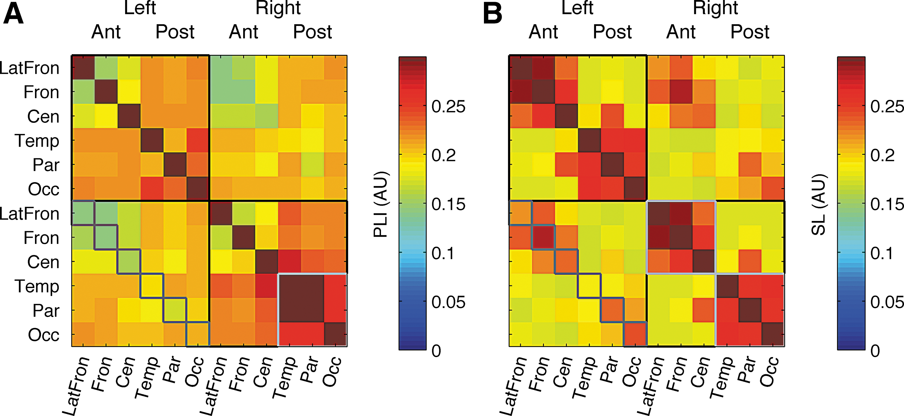
SL and PLI were compared both on a lead pair by lead pair basis and on average connectivity. When comparing the 66 lead-pair connectivity scores, SL and PLI correlations ranged from 0.111 for childhood age groups to 0.34 for adolescent age groups. Averaged across the whole scalp, the correlation between SL and PLI ranged from 0.30 to 0.65. This suggests that PLI and SL show overall different patterns of connectivity. The average connectivity pattern for SL and PLI is shown in Figure 1. Compared to PLI, SL showed stronger connectivity for nearby electrodes grouped into three clusters (frontal, central, and posterior). This may partly reflect volume conduction effects. SL also shows evidence of stronger connectivity across homologues than PLI. These are less likely to reflect volume conduction effects (Nunez et al., 1997) due to their relatively large interelectrode distance. Since PLI connectivity for homologues is relatively low, we can conclude that lateralized alpha sources mainly oscillate in phase. PLI connectivity showed a more evenly distributed pattern of connectivity than SL, but a parietal hub was visible, while the frontal cluster disappeared. In sum, average PLI connectivity taps partly into the same sources of individual variation as SL, however, the connectivity pattern differs for PLI and SL.

FIG. 1.

Connectivity matrices for PLI (A) and SL (B) for the adolescent age group (18 years). Matrices were converted to have matching averages and standard deviations to highlight the pattern rather than absolute differences in connectivity. Electrodes over left and right hemisphere (black boxes) as well as anterior (Lateral Frontal, Frontal, Central) and posterior (Temporal, Parietal, Occipital) areas are grouped. SL showed two clear clusters (light grey box) in either hemisphere. PLI showed a single posterior cluster (grey) that also connected well to the anterior areas. SL also showed stronger cross-hemisphere connectivity for homologues (dark grey boxes) compared to PLI. A repeated measures GEE model with repeated factor connectivity type (SL, PLI) and location pair (66 combinations) resulted in a highly significant interaction of type*location, χ ² = 7372.8, df = 65, p << 1.0 · 10⁻¹⁵. GEE, generalized estimating equations; PLI, phase lag index; SL, synchronization likelihood. Color images available online at www.liebertpub.com/brain

Increased order with increased LN

Figure 2 shows the dependency of MST graph parameters on LN. Each point in the scatterplot represents the MST graph values of a single individual. Note that most values fall close to the polynomial regression. A second-order polynomial fit was significant in all cases. The centrality measures and K_max showed a positive relationship with an upward curve as expected from random graph simulations (Boersma et al., 2013). Tree hierarchy (TH) also showed a positive dependence on LN, but with a downward curve, thus setting a limit to the effect of LN on TH. DI decreased with increasing LN in a linear manner, which may be expected since maximum and minimum values for DI may be derived analytically from LN (Stam, 2014). 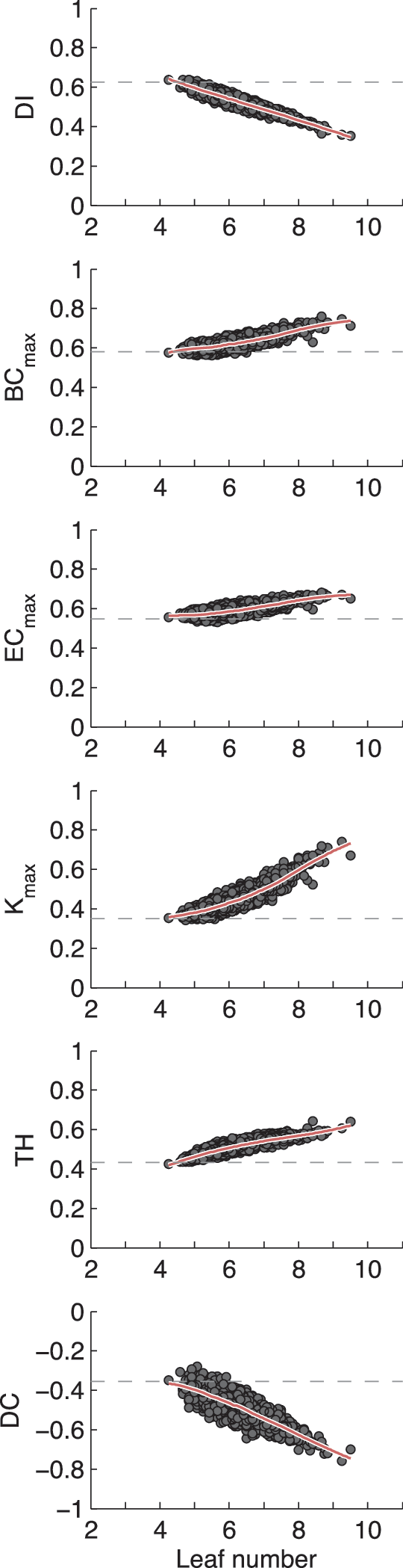DI will lie between \documentclass{aastex}\usepackage{amsbsy}\usepackage{amsfonts}\usepackage{amssymb}\usepackage{bm}\usepackage{mathrsfs}\usepackage{pifont}\usepackage{stmaryrd}\usepackage{textcomp}\usepackage{portland, xspace}\usepackage{amsmath, amsxtra}\pagestyle{empty}\DeclareMathSizes{10}{9}{7}{6}\begin{document}$$DI_{max} = N - LN + 1$$ \end{document} and \documentclass{aastex}\usepackage{amsbsy}\usepackage{amsfonts}\usepackage{amssymb}\usepackage{bm}\usepackage{mathrsfs}\usepackage{pifont}\usepackage{stmaryrd}\usepackage{textcomp}\usepackage{portland, xspace}\usepackage{amsmath, amsxtra}\pagestyle{empty}\DeclareMathSizes{10}{9}{7}{6}\begin{document}$$DI_{max} = 2 ( N - 1 ) / LN$$ \end{document} , where N is the number of nodes.

FIG. 2.

MST graph parameters covary with LN. From left to right on the x-axis, increased LN indicates increased hierarchical order and integration in the network. LN ranges from 2 (a linear configuration) to 11 (a star-like configuration) for a 12-vertex network, expressed in this study as a proportion from 0 to 1. Each plot contains an average MST graph parameter for each individual, plotted against average LN (averaged across multiple EEG epochs). The red line is a loess fit (50% width, second order). The dashed line indicates the average value obtained in 1000 graphs (n = 12) based on random signals. BC, betweenness centrality; DC, degree correlation; DI, diameter; EC, Eigenvector centrality; EEG, electroencephalography; LN, leaf number; MST, minimum spanning tree; TH, tree hierarchy. Color images available online at www.liebertpub.com/brain

PLI connectivity shows an inverted-U development

Figure 3 (top row) shows the results of average connectivity within the MST graph developing over age. Connectivity showed a pattern of development similar to those reported previously based on a different measure of connectivity (Smit et al., 2012). Top-left graph shows the development with loess fit (50% window size, second-order fit). The top-middle graph shows the same loess fit with bootstrap 95% confidence interval and reveals changes from childhood to early adulthood in average PLI, a decrease from 16 to 25. The omnibus test GEE model predicting average connectivity with age group as factor controlling for sex was highly significant, Wald χ ²(8) = 243.3, p = 4.5 · 10⁻⁴⁸. Post hoc comparisons with FDR adjustment revealed that significant increases were found from childhood to adolescence, but also between age groups 5 and 7. MST connectivity declined in the 57.5+ age group and reached significance in comparison to the adolescent and ∼40 age groups.

FIG. 3.

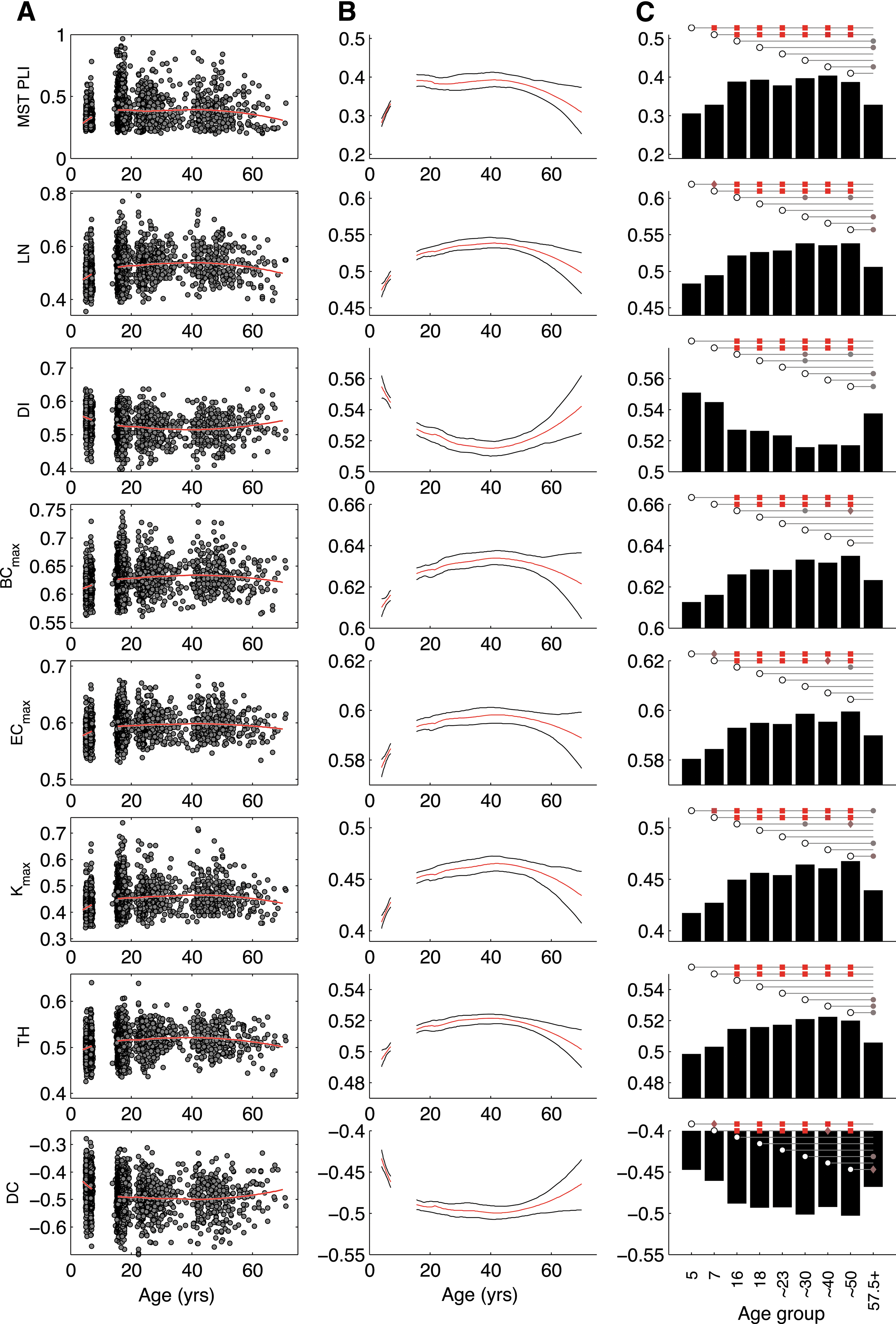
Age development plots for average connectivity strength (PLI) within the MST graph and MST network parameters of EEG alpha oscillations (6.0–13.0 Hz). (A) Large individual variation around loess smooth (50% width, second-order fit) was observed. Most parameters showed (inverted) a U-shaped development. (B) 95% confidence intervals were obtained by bootstrapping across families. (C) Group-wise comparison was corrected for residual correlation with robust SEs (see Methods section) and FDR corrected for the n*(n − 1)/2 comparisons (n = 9) and further multiplied by 2 to correct for the dimensionality of the data (as indicated by the PCA). Pairwise comparison was significant when an open circle is connected to a colored marker (grey/red). For example, age group 5 differed significantly in MST connectivity strength from ages 7, 16, 18, ∼23, ∼30, ∼40, and ∼50. Squares indicate the strongest effect (FDR corrected-p < 0.001) followed by diamonds (corrected-p < 0.01) and circles (corrected-p < 0.05). Color saturation indicates–log10(P), with gray values for corrected-p = 0.05 ranging to bright red for corrected-p = 10⁻⁷. FDR, false discovery rate; SEs, standard errors. Color images available online at www.liebertpub.com/brain

Connectivity patterns change with age

Although average PLI connectivity may change across different age groups, localized developmental differences may still occur. We assessed the connectivity between all possible pairs of signals and calculated change across the 9 age groups in a stepwise manner (i.e., 8 change values) expressed as rate per annum. Three-dimensional headplots were constructed using BrainNet Viewer (Xia et al., 2013) with approximate locations of the electrodes (Fig. 4 left column). The thickness of the edges was rescaled to average increase per annum making them comparable across headplots. Red colors indicate increase, blue decrease, and green indicates no change.

FIG. 4.

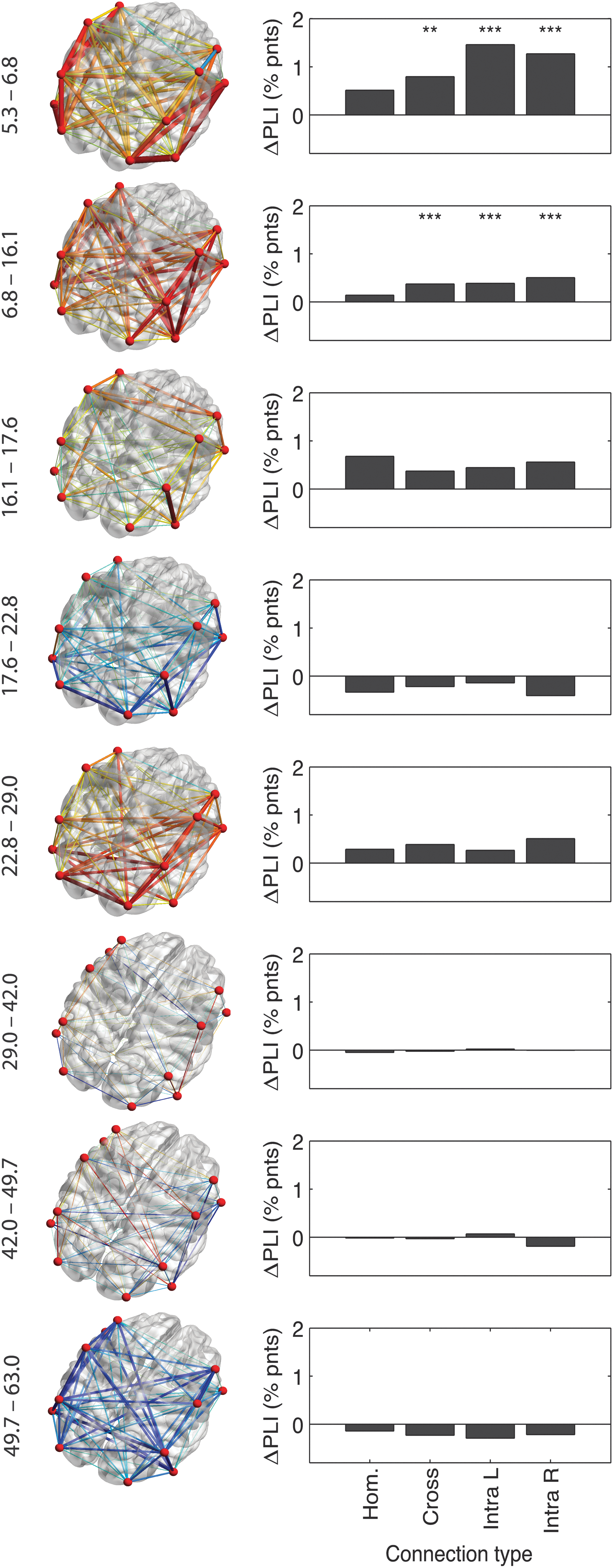
Localized development of connectivity strength. Left: 3D headplots of average change in PLI per year from one age group to the next (age groups 5, 7, 16, 18, ∼23, ∼30, ∼40, ∼50, 57.5+) from an elevated right posterior viewpoint. The location of maximal development is not stable, but changes with age. Actual ages of the age groups that are compared are shown on the left. Right: Separating edges into intrahemispheric left and right (Intra L, Intra R), contralateral homologues (Hom), and other cross-hemisphere (Cross) connections showed that childhood was marked by a clear intrahemispheric increase of connectivity, while later age groups showed no such strong prevalence or stronger increases in contralateral homologues (within adolescence). **p < 0.05, ***p < 0.001 after FDR correction at q = 0.05. Color images available online at www.liebertpub.com/brain

Changes within childhood were largely limited to intrahemispheric connections (Fig. 4 right column). Homologous (left–right lateralized) electrode pairs and other interhemispheric connections showed low PLI connectivity increase. From childhood to adolescence, both inter- and intrahemispheric connections showed increases, but homologues still showed less PLI change. In adolescence, a change is seen with homologues reaching the largest change. In later ages, reduction in connectivity strength is clearest in interhemispheric connections (other than homologues). In sum, the changes during childhood, adolescence, and middle-aged adulthood showed remarkable changes in topology. Clearly, the brain does not simply change connectivity, but changes the overall pattern of connectivity.

Reliability of MST parameters

Split-half reliability across two sets of eight epochs was corrected for the reduced time length in the eight compared to 16 epochs. Very high reliability for scalp-average PLI connectivity was obtained (0.96). Pairwise channel reliability ranged from r = 0.72 to 0.94. MST graph parameters were measured moderately reliably. Highest reliability was found for K_max (0.741). The other centrality measures showed lower reliability (BC_max: 0.587, EC_max: 0.592). LN, DI, and DC showed reliability of 0.71, 0.628, and 0.605, respectively.

An increasingly integrated network

Figure 3 also shows the development of MST graph parameters as scatterplot with loess fit (Fig. 3A), bootstrap of the loess fit with 95% confidence intervals (Fig. 3B), and pairwise testing of significance across age groups (Fig. 3C). Network parameters showed developmental trends highly comparable to connectivity. Cubic curves were not significant (absolute robust z < 1.4, ns). All quadratic terms were significant (absolute robust z > 6.44, p < 1.2E-10) with all parameters showing inverted-U shapes—except DI showed a U curve as expected.

The brain network of children showed a lower LN, indicating a more random network and less integrated organization. Increasing age resulted in an increased LN and a correspondingly increased BC_max, EC_max, and K_max. TH changed similarly in an inverted-u shape. DI and DC decreased. These findings are consistent with an increasing star-like organization and increased integration. The comparison of most measures showed significant change from 5 years of age to adolescence/adulthood with highly significant values (p < 0.0001, and p < 0.001 compared to age ∼40 for DC and EC_max). Age 7 showed a similar pattern. Both ages 5 and 7 generally showed no significant difference with the oldest age group (>57.5).

Older age (57.5+) was marked by a significant decrease for many parameters, although the effects were not very strong (p < 0.01). LN and TH decreased with older age compared to ages ∼30 to ∼50. Connectivity decreased only compared to age ∼40 (p < 0.01). The centrality measures showed less-consistent decrease, possibly due to a noisier variation.

Principal components reveal partly separate sources of variation

Since the developmental trends of connectivity and MST graph parameters showed markedly similar paths, we subjected the correlation matrix of four different measures for connectivity (homologous contralateral connectivity, other interhemispheric connectivity, and intrahemispheric connectivity left and right) and six MST-based graph parameters (LN, DI, BC_max, EC_max, K_max, DC) to an eigenvalue decomposition after selecting one random subject per family and regressing out the effects of age and sex. TH was excluded since it was based on two other parameters and therefore does not add information to the correlation matrix. Scores for DI and DC were inverted so as to enforce positive correlations. Figure 4 shows the results. The correlation matrix shows a clear clustering of connectivity versus MST graph parameters. The highest eigenvalue of 5.85 explained 58.5% of the variance, the second highest was 2.09 (20.9% variation). Both the correlation matrix (Fig. 5A) and the scree plot (Fig. 5C) strongly suggest a two-factor solution. After varimax rotation, MST parameters loaded strongly on the first component and PLI connectivity measures on the second (Fig. 5B). Figure 5D shows that the two components show different developmental patterns, with a much clearer U-curve for MST graph parameters, while PLI connectivity shows a decrease from adolescence to young adulthood. For these reasons, we conclude that MST graph parameters and PLI-based connectivity largely reflect different sources of variation in brain function with different developmental curves.

FIG. 5.

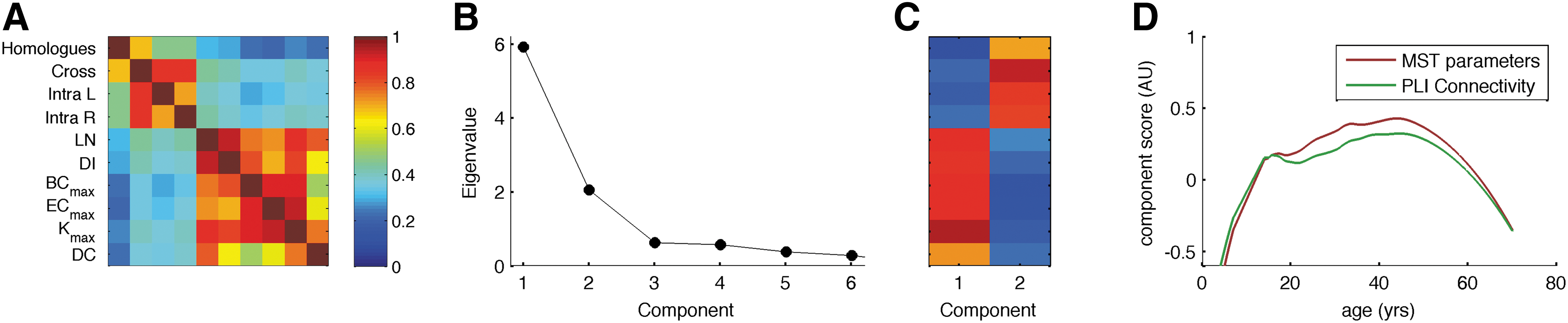
Principal Components Analysis of connectivity scores separated into contralateral homologues (Hom), other cross-hemispheric connections (Cross) intrahemisphere left (Intra L) and intrahemisphere right (Intra R), and MST graph measures. Note that TH was excluded as this measure is fully based on two other graph parameters (LN and BC_max). Positive correlations of DI and DC with other parameters were enforced by reversing scores. (A) The correlation matrix (corrected for age and sex) suggested two clusters, one for the four connectivity types, and one for the MST graph parameters. (B) The scree plot also strongly suggested two separate sources of variation. (C) The loading pattern for varimax-rotated two-component extraction showed clear separation of the connectivity and MST graph measures. (D) The varimax-rotated factor scores (corrected for sex) showed different developmental paths, suggesting that development differentially affects connectivity and MST graph parameters. Color images available online at www.liebertpub.com/brain

Preservation of properties in MST graphs

Twelve-node graphs are arguably insufficient to detect properties of the underlying network that has spatially much higher dimensionality. We therefore conducted an analysis on 39 datasets with 128-channel 4-min eyes-open resting EEG available in our laboratory. We refer to Smit and associates (2013) for more specifics on data recording. The cleaned data were filtered (8–13 Hz), epoched into sixteen 8-sec epochs, PLI connectivity calculated, MST parameters calculated, and averaged over the epochs. After that, we selected the 12 electrodes nearest to those in the current dataset, and recalculated PLI and MST parameters. The average PLI correlated highly (r = 0.97). K_max, DC, LN, and DI correlated moderately to highly (r = 0.48, r = 0.40, r = 0.70, and r = 0.61, respectively; all p < 0.011), indicating that a substantial proportion of interindividual variance is reflected in a very rudimentary 12-node representation of the initial 128-node network. BC_max and EC_max correlated nonsignificantly (r = 0.24), suggesting that maximum centrality measures are hardly preserved.

We additionally compared parameters derived from full 12-node graphs to those of MST graphs. Full graphs were thresholded graphs with a fixed average degree (K = 4.5) as calculated previously in this sample (Smit et al., 2012). The connectivity within the MST graphs correlated highly with connectivity in the full graphs (r = 0.93). K_max correlated r = 0.63, EC_max 0.46, and LN 0.44 between full and MST graphs. This confirms previously reported results that spanning trees conserve important node properties and properties on information flow (Kim et al., 2004; Tewarie et al., 2015). However, it also confirms that the overlap might not be perfect due to the arbitrary threshold selection (van Wijk et al., 2010).

Discussion

Our aim was to investigate whether the increased integration of the network observed from 5 to 7 years of age extends into adolescence and adulthood. The large and highly significant differences found in graph parameters and connectivity between childhood and adolescence/adulthood suggest that this is the case. We established that the life-span development of average connectivity between pairs of scalp-recorded signals closely mimics those reported previously (Smit et al., 2012). By using the PLI (Stam et al., 2007)—a measure that was designed to ignore volume conduction—we have found support that our previous findings using SL (Stam and van Dijk, 2002) have not been spurious. We hypothesize that the sparse electrode layout in our previous report may have been protective against detecting false synchronization (Smit et al., 2012).

Average connectivity within the MST measured with PLI showed strong increases within childhood and from childhood to adolescence. Our previous report on the same sample used SL as a measure of functional brain connectivity. Each measure is sensitive to different types of functional connectivity as evidenced by the different connectivity matrices they produce (Fig. 1). Even so, the current results show remarkable similarities with previous reported results. Both PLI and SL showed a strong increase from childhood to adolescence with effect sizes over r > 0.40 comparing age group 5 with other ages. PLI showed peak value at age 40 (Fig. 3, right column), with SL peaking at around age 50. This suggests that the previous results were quite robust against effects of volume conduction and common reference. However, the current results also differed from those reported previously. Connectivity measured using SL showed continuous and significant increases into late adulthood, whereas PLI connectivity showed a nonsignificant change (and a decrease from age 18 to ∼23). Moreover, the correlations between SL and PLI were generally low to moderate, suggesting that they reflect different sources of variation.

Several findings in the extant literature suggest that this increase in EEG functional connectivity depends on maturation of white brain matter, including myelinization. For example, it has been found that interhemispheric EEG connectivity measured by coherence has been related to diffusion tensor imaging diffusivity (Teipel et al., 2009) and T2 relaxation times in white matter in head injury, which arguably is related to neuronal membrane lesion (Thatcher et al., 1998). In addition, we have previously found that developmental curves for connectivity are highly consistent with the protracted development of white matter development: both connectivity and WMV showed peaks in middle age (Allen et al., 2005; Bartzokis et al., 2001; Benes et al., 1994; Good et al., 2002; Walhovd et al., 2005a, 2005b; Westlye et al., 2010). Moreover, a moderate correlation was found between WMV and connectivity. Because PLI reduces the effects of spurious connectivity in the brain based on volume conduction and common reference, these results seem to further strengthen the idea that functional connectivity in the resting state reflects the strength of anatomical connectivity between distant brain areas. It is not expected that changes in head circumference are a spurious explanation for the observed changes in functional connectivity and resulting changes in the MST network. At the age of 5, the head has reached 90% of its final size (Rollins et al., 2010). Moreover, effects on volume conduction due to head growth are likely to scale with the brain and not produce relative changes in (relative) conductive properties of the brain/skull/scalp. Global changes in volume conduction induced by head circumference increase seem inconsistent with the regional changes in connectivity as revealed in Figure 4. Finally, we have previously found that signal strength (oscillatory power) is larger in childhood than in adulthood (Smit et al., 2012), which would indicate that S/N ratios decrease with age. Reduced S/N should result in noisier PLI estimates and graphs closer to noise, which is the opposite of what was observed. More likely, synaptic pruning and white matter development caused the increase of connectivity, resulting in greater connectivity and complexity even at larger distances. Functionally, brain regions come “closer” together during brain size increase.

Arguably, MST graphs are more comparable across groups than thresholded graphs (Stam, 2014; van Wijk et al., 2010). Graph parameters derived from the MST graph showed evidence for change in the level of integration. All MST parameters show an inverted-U curve (and a U curve for diameter). The backbone graph in the human brain activity moved from a line to a more star-like configuration during development. In later age, a return to a more line-like configuration was found. For all, but the centrality measures, these resulted in significant drops for age group 57.5+ compared to ages 30 and 50. Importantly, principal components analysis showed that MST graph parameters reflected different sources of variation compared to PLI connectivity. Clearly, not just the average connectivity, but the connectivity pattern changes. Note that we observed that MST graph parameters showed a more star-like configuration than random graphs (Fig. 1). In this sense, the observed developmental changes showed a move from random networks toward more integrated networks, and more random networks in later life. This, too, is consistent with previous observations of life-span development in the same sample (Boersma et al., 2010; Smit et al., 2010, 2012).

The current EEG dataset was limited to a small number of EEG signals (n = 12). The signals are linear combinations of the neural generators they project to the scalp location of the electrodes. Although the PLI algorithm disregards spurious connectivity of neural sources that project to multiple electrodes, it is clear that many sources contribute to a signal electrode. Therefore, each signal represents the activity of a large area in proximity of the electrode. We therefore analyzed high-density recordings for PLI and MST parameters, downsampled spatially to 12 channels, and analyzed PLI and MST parameters again. Average connectivity was well represented in the reduced 12-node network. In addition, many MST parameters were also (partially) preserved in the 10-fold reduced networks (notably, K_max, DC, and LN). Note that this reduction includes an increased measurement error. Therefore, we conclude that the observed developmental changes in 12-node networks suggest that high-density measurements could, likely with much higher power, detect a similar change.

The results make MST graph parameters highly suitable as biomarkers for the development in early life and cognitive decline associated with older age. Follow-up studies could target the genetic variants that have been linked to neuronal change such as myelination. In addition, studies could investigate how genetic variants exert their influence in cognitive decline or Alzheimer's disease (e.g., apolipoprotein E gene [APOE], clusterin gene [CLU/APOJ], and phosphatidylinositol binding clathrin assembly protein [PICALM]) (Harold et al., 2009; Hollingworth et al., 2011; Lambert et al., 2013). Carriers of the APOE \documentclass{aastex}\usepackage{amsbsy}\usepackage{amsfonts}\usepackage{amssymb}\usepackage{bm}\usepackage{mathrsfs}\usepackage{pifont}\usepackage{stmaryrd}\usepackage{textcomp}\usepackage{portland, xspace}\usepackage{amsmath, amsxtra}\pagestyle{empty}\DeclareMathSizes{10}{9}{7}{6}\begin{document}$$\epsilon 4$$ \end{document} allele have an increased risk for forming beta-amyloid plaques; during prion-like aggregation, damage to neurons is done by oxidative stress, resulting in brain atrophy. This loss significantly reduces the number of neurons available for connectivity such as that seen in mild cognitive impairment and Alzheimer's disease (Jelic et al., 1997; Tóth et al., 2014), and may additionally result in the loss of integration in the MST network. Likewise, clusterin (CLU/APOJ) is involved in the clearance by binding to beta-amyloid resulting in variability in neurodegeneration (Desikan et al., 2014; Mengel-From et al., 2013) and could have similar effects on connectivity and connectivity patterns. PICALM highlights the need to investigate inflammatory pathways (Perry et al., 2010). From the current results, we expect that connectivity loss will prove to be nonrandom, resulting in reduced integration due to specific attacks on central nodes (He et al., 2009; Stam et al., 2009).

In developmental neurobiology, the dichotomy into long and short projection distances may be essential. In an fMRI study, it was shown that decreased short-range connectivity concurs with increased long-range connectivity. Local connections in a cognitive control network become less diffuse with development from 10 to 22 years of age, which is accompanied by an increased long-distance functional connectivity (Kelly et al., 2009). Similar findings of changes in (long-distance) connectivity have been reported (Dosenbach et al., 2010; Fair et al., 2009; Supekar et al., 2009). The present results extend these findings in showing that from childhood to adulthood, brain networks move from less to more integrated graphs (Fig. 2). Since network parameters may be relevant predictors of cognitive performance (Micheloyannis et al., 2006; Tewarie et al., 2014; van den Heuvel et al., 2009) and are disrupted in neurological disorders (Stam et al., 2009, 2014; Tewarie et al., 2014; van Dellen et al., 2014), we can hypothesize that the increasingly integrated network topology is essential to the large developmental changes in human cognitive performance during the same period. Indeed, a more integrated network was predictive of better cognitive performance in MS patients (Tewarie et al., 2014). Cognitive performance correlated with a larger decrease in network integration in Parkinson's patients (Dubbelink et al., 2014). Whether these findings generalize to the normal population may be addressed in future investigations.

In conclusion, brain connectivity measured by the PLI shows large changes over the lifespan. These changes largely corroborate the earlier findings that the connection strength increases during development (Hagmann et al., 2010; Smit et al., 2010, 2012). Since PLI is less sensitive to volume conduction by ignoring the zero and π phase differences between signal pairs (Stam et al., 2007), developmental changes are therefore unlikely to reflect changes in conductive properties across age groups. The use of the MST backbone graph aimed to solve the problem that graph measures may not be compared across different sizes and degree distributions (van Wijk et al., 2010). However, MST graphs confirmed that brain matures across the lifespan and shows changes in structure both in the development in childhood and during aging in later life. These findings corroborate our earlier findings that the network shows reduced randomness from childhood to young adulthood (Boersma et al., 2010, 2013; Schutte et al., 2013; Smit et al., 2010, 2012).

Footnotes

Acknowledgments

This work was supported by grants Twin-family database for behavior genetics and genomics studies (NWO 480-04-004) to D.B., Genotype/phenotype database for behavior genetics and genetic epidemiological studies (NWO 911-09-032) to D.B., European Research Council (ERC-230374) to D.B., BBR Foundation (NARSAD) Young Investigator grant 21668 to D.S., NWO/MagW VENI-451-08-026 to D.S., VU University VU-USF 96/22 to D.B., Human Frontiers of Science Program RG0154/1998-B to D.B., and E.d.G., Netherlands Organization for Scientific Research, NWO/SPI 56-464-14192 to D.B.

Author Disclosure Statement

No competing financial interests exist.

References

Albert

, Jeong

, Barabási

A-L

. 2000. Error and attack tolerance of complex networks. Nature, 406:378–382.

Allen

, Bruss

, Brown

, Damasio

. 2005. Normal neuroanatomical variation due to age: the major lobes and a parcellation of the temporal region. Neurobiol Aging, 26:1245–1260.

Bartzokis

, Beckson

, Lu

, Nuechterlein

, Edwards

, Mintz

. 2001. Age-related changes in frontal and temporal lobe volumes in men: a magnetic resonance imaging study. Arch Gen Psychiatry, 58:461–465.

Benes

, Turtle

, Khan

, Farol

. 1994. Myelination of a key relay zone in the hippocampal formation occurs in the human brain during childhood, adolescence, and adulthood. Arch Gen Psychiatry, 51:477.

Benjamini

, Hochberg

. 1995. Controlling the false discovery rate: a practical and powerful approach to multiple testing. J R Stat Soc Ser B (Methodological), 57:289–300.

Boersma

, Smit

, Boomsma

, De Geus

, Delemarre-van de Waal

, Stam

. 2013. Growing trees in child brains: graph theoretical analysis of electroencephalography-derived minimum spanning tree in 5-and 7-year-old children reflects brain maturation. Brain Connect, 3:50–60.

Boersma

, Smit

DJA

, de Bie

HMA

, Van Baal

GCM

, Boomsma

, de Geus

EJC

, Delemarre-van de Waal

, Stam

. 2010. Network analysis of resting state EEG in the developing young brain: structure comes with maturation. Hum Brain Mapp, 32:413–425.

Britz

, Van De Ville

, Michel

. 2010. BOLD correlates of EEG topography reveal rapid resting-state network dynamics. Neuroimage, 52:1162–1170.

Bullmore

, Sporns

. 2009. Complex brain networks: graph theoretical analysis of structural and functional systems. Nat Rev Neurosci, 10:186–198.

10.

Casey

, Giedd

, Thomas

. 2000. Structural and functional brain development and its relation to cognitive development. Biol Psychol, 54:241–257.

11.

Çiftçi

. 2011. Minimum spanning tree reflects the alterations of the default mode network during Alzheimer's disease. Ann Biomed Eng, 39:1493–1504.

12.

Courchesne

, Chisum

, Townsend

, Cowles

, Covington

, Egaas

, Harwood

, Hinds

, Press

. 2000. Normal brain development and aging: quantitative analysis at in vivo MR imaging in healthy volunteers. Radiology, 216:672–682.

13.

Damoiseaux

, Rombouts

SARB

, Barkhof

, Scheltens

, Stam

, Smith

, Beckmann

. 2006. Consistent resting-state networks across healthy subjects. Proc Natl Acad Sci U S A, 103:13848–13853.

14.

de Haan

, Pijnenburg

YAL

, Strijers

RLM

, van der Made

, van der Flier

, Scheltens

, Stam

. 2009. Functional neural network analysis in frontotemporal dementia and Alzheimer's disease using EEG and graph theory. BMC Neurosci, 10:101.

15.

Delorme

, Makeig

. 2004. EEGLAB: an open source toolbox for analysis of single-trial EEG dynamics including independent component analysis. J Neurosci Methods, 134:9–21.

16.

Desikan

, Thompson

, Holland

, et al. 2014. THe role of clusterin in amyloid-β–associated neurodegeneration. JAMA Neurol, 71:180–187.

17.

Dosenbach

NUF

, Nardos

, Cohen

, Fair

, Power

, Church

, Nelson

, Wig

, Vogel

, Lessov-Schlaggar

, Barnes

, Dubis

, Feczko

, Coalson

, Pruett

, Barch

, Petersen

, Schlaggar

. 2010. Prediction of individual brain maturity using fMRI. Science, 329:1358–1361.

18.

Dubbelink

KTEO

, Hillebrand

, Stoffers

, Deijen

, Twisk

JWR

, Stam

, Berendse

. 2014. Disrupted brain network topology in Parkinson's disease: a longitudinal magnetoencephalography study. Brain, 137:197–207.

19.

Fair

, Cohen

, Dosenbach

NUF

, Church

, Miezin

, Barch

, Raichle

, Petersen

, Schlaggar

. 2008. The maturing architecture of the brain's default network. Proc Natl Acad Sci U S A, 105:4028–4032.

20.

Fair

, Cohen

, Power

, Dosenbach

NUF

, Church

, Miezin

, Schlaggar

, Petersen

. 2009. Functional brain networks develop from a “Local to Distributed” organization. PLoS Comput Biol, 5:e1000381.

21.

Fransson

, Aden

, Blennow

, Lagercrantz

. 2010. The functional architecture of the infant brain as revealed by resting-state fMRI. Cereb Cortex, 21:145–154.

22.

Giedd

, Blumenthal

, Jeffries

, Castellanos

, Liu

, Zijdenbos

, Paus

, Evans

, Rapoport

. 1999. Brain development during childhood and adolescence: a longitudinal MRI study. Nat Neurosci, 2:861–863.

23.

Gogtay

, Giedd

, Lusk

, Hayashi

, Greenstein

, Vaituzis

, Nugent

, Herman

, Clasen

, Toga

, Rapoport

, Thompson

. 2004. Dynamic mapping of human cortical development during childhood through early adulthood. Proc Natl Acad Sci U S A, 101:8174–8179.

24.

Good

, Johnsrude

, Ashburner

, Henson

RNA

, Fristen

, Frackowiak

RSJ

. 2002. A voxel-based morphometric study of ageing in 465 normal adult human brains. In Biomedical Imaging, 5th IEEE EMBS International Summer School,, 2002, p. 16; DOI:10.1109/SSBI.2002.1233974

25.

Hagmann

, Sporns

, Madan

, Cammoun

, Pienaar

, Wedeen

, Meuli

, Thiran

J-P

, Grant

. 2010. White matter maturation reshapes structural connectivity in the late developing human brain. Proc Natl Acad Sci U S A, 107:19067–19072.

26.

Hanlon

, Thatcher

, Cline

. 1999. Gender differences in the development of EEG coherence in normal children. Dev Neuropsychol, 16:479–506.

27.

Harold

, Abraham

, Hollingworth

, Sims

, Gerrish

, Hamshere

, Pahwa

, Moskvina

, Dowzell

, Williams

, Jones

, Thomas

, Stretton

, Morgan

, Lovestone

, Powell

, Proitsi

, Lupton

, Brayne

, Rubinsztein

, Gill

, Lawlor

, Lynch

, Morgan

, Brown

, Passmore

, Craig

, McGuinness

, Todd

, Holmes

, Mann

, Smith

, Love

, Kehoe

, Hardy

, Mead

, Fox

, Rossor

, Collinge

, Maier

, Jessen

, Schürmann

, Heun

, van den Bussche

, Heuser

, Kornhuber

, Wiltfang

, Dichgans

, Frölich

, Hampel

, Hüll

, Rujescu

, Goate

, Kauwe

JSK

, Cruchaga

, Nowotny

, Morris

, Mayo

, Sleegers

, Bettens

, Engelborghs

, De Deyn

, Van Broeckhoven

, Livingston

, Bass

, Gurling

, McQuillin

, Gwilliam

, Deloukas

, Al-Chalabi

, Shaw

, Tsolaki

, Singleton

, Guerreiro

, Mühleisen

, Nöthen

, Moebus

, Jöckel

K-H

, Klopp

, Wichmann

H-E

, Carrasquillo

, Pankratz

, Younkin

, Holmans

, O'Donovan

, Owen

, Williams

. 2009. Genome-wide association study identifies variants at CLU and PICALM associated with Alzheimer's disease. Nat Genet, 41:1088–1093.

28.

, Chen

, Gong

, Evans

. 2009. Neuronal networks in Alzheimer's disease. Neuroscientist, 15:333–350.

29.

Heuvel

, van den Mandl

RCW

, Stam

, Kahn

, Pol

HEH

. 2010. Aberrant frontal and temporal complex network structure in schizophrenia: a graph theoretical analysis. J Neurosci, 30:15915–15926.

30.

Hollingworth

, Harold

, Sims

, Gerrish

, Lambert

J-C

, Carrasquillo

, Abraham

, Hamshere

, Pahwa

, Moskvina

, Dowzell

, Jones

, Stretton

, Thomas

, Richards

, Ivanov

, Widdowson

, Chapman

, Lovestone

, Powell

, Proitsi

, Lupton

, Brayne

, Rubinsztein

, Gill

, Lawlor

, Lynch

, Brown

, Passmore

, Craig

, McGuinness

, Todd

, Holmes

, Mann

, Smith

, Beaumont

, Warden

, Wilcock

, Love

, Kehoe

, Hooper

, Vardy

ERLC

, Hardy

, Mead

, Fox

, Rossor

, Collinge

, Maier

, Jessen

, Rüther

, Schürmann

, Heun

, Kölsch

, van den Bussche

, Heuser

, Kornhuber

, Wiltfang

, Dichgans

, Frölich

, Hampel

, Gallacher

, Hüll

, Rujescu

, Giegling

, Goate

, Kauwe

JSK

, Cruchaga

, Nowotny

, Morris

, Mayo

, Sleegers

, Bettens

, Engelborghs

, De Deyn

, Van Broeckhoven

, Livingston

, Bass

, Gurling

, McQuillin

, Gwilliam

, Deloukas

, Al-Chalabi

, Shaw

, Tsolaki

, Singleton

, Guerreiro

, Mühleisen

, Nöthen

, Moebus

, Jöckel

K-H

, Klopp

, Wichmann

H-E

, Pankratz

, Sando

, Aasly

, Barcikowska

, Wszolek

, Dickson

, Graff-Radford

, Petersen

, the Alzheimer's Disease Neuroimaging Initiative, van Duijn

, Breteler

MMB

, Ikram

, DeStefano

, Fitzpatrick

, Lopez

, Launer

, Seshadri

, Charge Consortium. Berr

, Campion

, Epelbaum

, Dartigues

J-F

, Tzourio

, Alpérovitch

, Lathrop

, Eadi1 Consortium, Feulner

, Friedrich

, Riehle

, Krawczak

, Schreiber

, Mayhaus

, Nicolhaus

, Wagenpfeil

, Steinberg

, Stefansson

, Snædal

, Björnsson

, Jonsson

, Chouraki

, Genier-Boley

, Hiltunen

, Soininen

, Combarros

, Zelenika

, Delepine

, Bullido

, Pasquier

, Mateo

, Frank-Garcia

, Porcellini

, Hanon

, Coto

, Alvarez

, Bosco

, Siciliano

, Mancuso

, Panza

, Solfrizzi

, Nacmias

, Sorbi

, Bossù

, Piccardi

, Arosio

, Annoni

, Seripa

, Pilotto

, Scarpini

, Galimberti

, Brice

, Hannequin

, Licastro

, Jones

, Holmans

, Jonsson

, Riemenschneider

, Morgan

, Younkin

, Owen

, O'Donovan

, Amouyel

, Williams

. 2011. Common variants at ABCA7, MS4A6A/MS4A4E, EPHA1, CD33 and CD2AP are associated with Alzheimer's disease. Nat Genet, 43:429–435.

31.

Huttenlocher

. 1979. Synaptic density in human frontal cortex—developmental changes and effects of aging. Brain Res, 163:195–205.

32.

Huttenlocher

, Dabholkar

. 1997. Regional differences in synaptogenesis in human cerebral cortex. J Comp Neurol, 387:167–178.

33.

Huttenlocher

, de Courten

. 1987. The development of synapses in striate cortex of man. Hum Neurobiol, 6:1–9.

34.

Jelic

, Julin

, Shigeta

, Nordberg

, Lannfelt

, Winblad

, Wahlund

L-O

. 1997. Apolipoprotein E ɛ4 allele decreases functional connectivity in Alzheimer's disease as measured by EEG coherence. J Neurol Neurosurg Psychiatry, 63:59–65.

35.

Kelly

, Di Martino

, Uddin

, Shehzad

, Gee

, Reiss

, Margulies

, Castellanos

, Milham

. 2009. Development of anterior cingulate functional connectivity from late childhood to early adulthood. Cereb Cortex, 19:640.

36.

Kim

D-H

, Noh

, Jeong

. 2004. Scale-free trees: the skeletons of complex networks. Phys Rev E, 70:046126.

37.

Kruskal

Jr.

1956. On the shortest spanning subtree of a graph and the traveling salesman problem. Proc Am Math Soc, 7:48–50.

38.

Lambert

J-C

, Ibrahim-Verbaas

, Harold

, Naj

, Sims

, Bellenguez

, Jun

, DeStefano

, Bis

, Beecham

, Grenier-Boley

, Russo

, Thornton-Wells

, Jones

, Smith

, Chouraki

, Thomas

, Ikram

, Zelenika

, Vardarajan

, Kamatani

, Lin

C-F

, Gerrish

, Schmidt

, Kunkle

, Dunstan

, Ruiz

, Bihoreau

M-T

, Choi

S-H

, Reitz

, Pasquier

, Hollingworth

, Ramirez

, Hanon

, Fitzpatrick

, Buxbaum

, Campion

, Crane

, Baldwin

, Becker

, Gudnason

, Cruchaga

, Craig

, Amin

, Berr

, Lopez

, De Jager

, Deramecourt

, Johnston

, Evans

, Lovestone

, Letenneur

, Morón

, Rubinsztein

, Eiriksdottir

, Sleegers

, Goate

, Fiévet

, Huentelman

, Gill

, Brown

, Kamboh

, Keller

, Barberger-Gateau

, McGuinness

, Larson

, Green

, Myers

, Dufouil

, Todd

, Wallon

, Love

, Rogaeva

, Gallacher

St. , George-Hyslop

, Clarimon

, Lleo

, Bayer

, Tsuang

, Yu

, Tsolaki

, Bossù

, Spalletta

, Proitsi

, Collinge

, Sorbi

, Sanchez-Garcia

, Fox

, Hardy

, Naranjo

MCD

, Bosco

, Clarke

, Brayne

, Galimberti

, Mancuso

, Matthews

, European Alzheimer's Disease Initiative (EADI), Genetic and Environmental Risk in Alzheimer's Disease (GERAD), Alzheimer's Disease Genetic Consortium (ADGC), Cohorts for Heart and Aging Research in Genomic Epidemiology (CHARGE), Moebus

, Mecocci

, Del Zompo

, Maier

, Hampel

, Pilotto

, Bullido

, Panza

, Caffarra

, Nacmias

, Gilbert

, Mayhaus

, Lannfelt

, Hakonarson

, Pichler

, Carrasquillo

, Ingelsson

, Beekly

, Alvarez

, Zou

, Valladares

, Younkin

, Coto

, Hamilton-Nelson

, Gu

, Razquin

, Pastor

, Mateo

, Owen

, Faber

, Jonsson

, Combarros

, O'Donovan

, Cantwell

, Soininen

, Blacker

, Mead

, Mosley

Jr. , Bennett

, Harris

, Fratiglioni

, Holmes

, de Bruijn

RFAG

, Passmore

, Montine

, Bettens

, Rotter

, Brice

, Morgan

, Foroud

, Kukull

, Hannequin

, Powell

, Nalls

, Ritchie

, Lunetta

, Kauwe

JSK

, Boerwinkle

, Riemenschneider

, Boada

, Hiltunen

, Martin

, Schmidt

, Rujescu

, Wang

L-S

, Dartigues

J-F

, Mayeux

, Tzourio

, Hofman

, Nöthen

, Graff

, Psaty

, Jones

, Haines

, Holmans

, Lathrop

, Pericak-Vance

, Launer

, Farrer

, van Duijn

, Van Broeckhoven

, Moskvina

, Seshadri

, Williams

, Schellenberg

, Amouyel

. 2013. Meta-analysis of 74,046 individuals identifies 11 new susceptibility loci for Alzheimer's disease. Nat Genet, 45:1452–1458.

39.

Lee

, Kim

, Jung

K-Y

. 2006. Classification of epilepsy types through global network analysis of scalp electroencephalograms. Phys Rev E, 73:041920.

40.

Lenroot

, Giedd

. 2006. Brain development in children and adolescents: insights from anatomical magnetic resonance imaging. Neurosci Biobehav Rev, 30:718–729.

41.

Mantini

, Perrucci

, Del Gratta

, Romani

, Corbetta

. 2007. Electrophysiological signatures of resting state networks in the human brain. Proc Natl Acad Sci U S A, 104:13170–13175.

42.

Mengel-From

, Thinggaard

, Lindahl-Jacobsen

, McGue

, Christensen

, Christiansen

. 2013. CLU genetic variants and cognitive decline among elderly and oldest old. PLoS One, 8:e79105.

43.

Menon

. 2011. Large-scale brain networks and psychopathology: a unifying triple network model. Trends Cogn Sci, 15:483–506.

44.

Meunier

, Achard

, Morcom

, Bullmore

. 2009. Age-related changes in modular organization of human brain functional networks. Neuroimage, 44:715–723.

45.

Micheloyannis

, Pachou

, Stam

, Vourkas

, Erimaki

, Tsirka

. 2006. Using graph theoretical analysis of multi channel EEG to evaluate the neural efficiency hypothesis. Neurosci Lett, 402:273–277.

46.

Minică

, Boomsma

, Vink

, Dolan

. 2014. MZ twin pairs or MZ singletons in population family-based GWAS? More power in pairs. Mol Psychiatry, 19:1154–1155.

47.

Musso

, Brinkmeyer

, Mobascher

, Warbrick

, Winterer

. 2010. Spontaneous brain activity and EEG microstates. A novel EEG/fMRI analysis approach to explore resting-state networks. Neuroimage, 52:1149–1161.

48.

Nunez

, Srinivasan

. 2006. Electric Fields of the Brain: The Neurophysics of EEG. New York: Oxford University. Press.

49.

Nunez

, Srinivasan

, Westdorp

, Wijesinghe

, Tucker

, Silberstein

, Cadusch

. 1997. EEG coherency: I: statistics, reference electrode, volume conduction, Laplacians, cortical imaging, and interpretation at multiple scales. Electroencephalogr Clin Neurophysiol, 103:499–515.

50.

Paus

. 2005. Mapping brain maturation and cognitive development during adolescence. Trends Cogn Sci, 9:60–68.

51.

Paus

, Collins

, Evans

, Leonard

, Pike

, Zijdenbos

. 2001. Maturation of white matter in the human brain: a review of magnetic resonance studies. Brain Res Bull, 54:255–266.

52.

Perry

, Nicoll

JAR

, Holmes

. 2010. Microglia in neurodegenerative disease. Nat Rev Neurol, 6:193–201.

53.

Pivik

, Broughton

, Coppola

, Davidson

, Fox

, Nuwer

. 1993. Guidelines for the recording and quantitative analysis of electroencephalographic activity in research contexts. Psychophysiology, 30:547–558.

54.

Power

, Fair

, Schlaggar

, Petersen

. 2010. The development of human functional brain networks. Neuron, 67:735–748.

55.

Rollins

, Collins

, Holden

. 2010. United States head circumference growth reference charts: birth to 21 years. J Pediatr, 156:907–913.e2.

56.

Rubinov

, Sporns

. 2010. Complex network measures of brain connectivity: uses and interpretations. NeuroImage, 52:1059–1069.

57.

Schutte

, Hansell

, de Geus

, Martin

, Wright

, Smit

. 2013. Heritability of resting state EEG functional connectivity patterns. Twin Res Hum Genet, 16:962–969.

58.

Serrano

MÁ

, Boguñá

, Vespignani

. 2009. Extracting the multiscale backbone of complex weighted networks. Proc Natl Acad Sci U S A, 106:6483–6488.

59.

Shaw

, Greenstein

, Lerch

, Clasen

, Lenroot

, Gogtay

, Evans

, Rapoport

, Giedd

. 2006. Intellectual ability and cortical development in children and adolescents. Nature, 440:676–679.

60.

Smit

DJA

, Boersma

, Beijsterveldt

CEM

, Posthuma

, Boomsma

, Stam

, Geus

EJC

. 2010. Endophenotypes in a dynamically connected brain. Behav Genet, 40:167–177.

61.

Smit

DJA

, Boersma

, Schnack

, Micheloyannis

, Boomsma

, Hulshoff Pol

, Stam

, de Geus

EJC

. 2012. The brain matures with stronger functional connectivity and decreased randomness of its network. PLoS One, 7:e36896.

62.

Smit

, Linkenkaer-Hansen

, de Geus

. 2013. Long-range temporal correlations in resting-state alpha oscillations predict human timing-error dynamics. J Neurosci, 33:11212–11220.

63.

Sporns

. 2014. Contributions and challenges for network models in cognitive neuroscience. Nat Neurosci, 17:652–660.

64.

Stam

. 2014. Modern network science of neurological disorders. Nat Rev Neurosci, 15:683–695.

65.

Stam

, de Haan

, Daffertshofer

, Jones

, Manshanden

, van Cappellen van Walsum

, Montez

, Verbunt

JPA

, de Munck

, van Dijk

, Berendse

, Scheltens

. 2009. Graph theoretical analysis of magnetoencephalographic functional connectivity in Alzheimer's disease. Brain, 132:213–224.

66.

Stam

, Nolte

, Daffertshofer

. 2007. Phase lag index: assessment of functional connectivity from multi channel EEG and MEG with diminished bias from common sources. Hum Brain Mapp, 28:1178–1193.

67.

Stam

, Tewarie

, Van Dellen

, van Straaten

ECW

, Hillebrand

, Van Mieghem

. 2014. The trees and the forest: characterization of complex brain networks with minimum spanning trees. Int J Psychophysiol, 92:129–138.

68.

Stam

, van Dijk

. 2002. Synchronization likelihood: an unbiased measure of generalized synchronization in multivariate data sets. Phys D, 163:236–251.

69.

Supekar

, Musen

, Menon

. 2009. Development of large-scale functional brain networks in children. PLoS Biol, 7:e1000157.

70.

Teipel

, Pogarell

, Meindl

, Dietrich

, Sydykova

, Hunklinger

, Georgii

, Mulert

, Reiser

, Möller

. 2009. Regional networks underlying interhemispheric connectivity: an EEG and DTI study in healthy ageing and amnestic mild cognitive impairment. Hum Brain Mapp, 30:2098–2119.

71.

Tewarie

, Hillebrand

, Schoonheim

, van Dijk

, Geurts

JJG

, Barkhof

, Polman

, Stam

. 2014. Functional brain network analysis using minimum spanning trees in multiple sclerosis: an MEG source-space study. NeuroImage, 88:308–318.

72.

Tewarie

, van Dellen

, Hillebrand

, Stam

. 2015. The minimum spanning tree: an unbiased method for brain network analysis. NeuroImage, 104:177–188.

73.

Thatcher

, Biver

, McAlaster

, Salazar

. 1998. Biophysical linkage between MRI and EEG coherence in closed head injury. Neuroimage, 8:307–326.

74.

Tijms

, Wink

, de Haan

, van der Flier

, Stam

, Scheltens

, Barkhof

. 2013. Alzheimer's disease: connecting findings from graph theoretical studies of brain networks. Neurobiol Aging, 34:2023–2036.

75.

Tóth

, File

, Boha

, Kardos

, Hidasi

, Gaál

, Csibri

, Salacz

, Stam

, Molnár

. 2014. EEG network connectivity changes in mild cognitive impairment—preliminary results. Int J Psychophysiol, 92:1–7.

76.

van Dellen

, Douw

, Hillebrand

, de Witt Hamer

, Baayen

, Heimans

, Reijneveld

, Stam

. 2014. Epilepsy surgery outcome and functional network alterations in longitudinal MEG: a minimum spanning tree analysis. NeuroImage, 86:354–363.

77.

van den Heuvel

, Stam

, Kahn

, Hulshoff Pol

. 2009. Efficiency of functional brain networks and intellectual performance. J Neurosci, 29:7619–7624.

78.

van Wijk

BCM

, Stam

, Daffertshofer

. 2010. Comparing brain networks of different size and connectivity density using graph theory. PLoS One, 5:e13701.

79.

Walhovd

, Fjell

, Reinvang

, Lundervold

, Dale

, Eilertsen

, Quinn

, Salat

, Makris

, Fischl

. 2005a. Effects of age on volumes of cortex, white matter and subcortical structures. Neurobiol Aging, 26:1261–1270.

80.

Walhovd

, Fjell

, Reinvang

, Lundervold

, Dale

, Quinn

, Salat

, Makris

, Fischl

. 2005b. Neuroanatomical aging: universal but not uniform. Neurobiol Aging, 26:1279–1282.

81.

Watts

, Strogatz

. 1998. Collective dynamics of/‘small-world/’ networks. Nature, 393:440–442.

82.

Westlye

, Walhovd

, Dale

, Bjørnerud

, Due-Tønnessen

, Engvig

, Grydeland

, Tamnes

, Østby

, Fjell

. 2010. Life-span changes of the human brain white matter: diffusion tensor imaging (DTI) and volumetry. Cereb Cortex, 20:2055–2068.

83.

Xia

, Wang

, He

. 2013. BrainNet viewer: a network visualization tool for human brain connectomics. PLoS One, 8:e68910.

84.

Zhao

, Liu

, Wang

, Liu

, Xi

, Guo

, Jiang

, Wang

. 2012. Disrupted small-world brain networks in moderate Alzheimer's disease: a resting-state fMRI study. PLoS One, 7:e33540.