Reliability of Functional Connectivity of Electroencephalography Applying Microstate-Segmented Versus Classical Calculation of Phase Lag Index

Abstract

Connectivity analysis characterizes normal and altered brain function, for example, using the phase lag index (PLI), which is based on phase relations. However, reliability of PLI over time is limited, especially for single- or regional-link analysis. One possible cause is repeated changes of network configuration during registration. These network changes may be associated with changes of the surface potential fields, which can be characterized by microstate analysis. Microstate analysis describes repeating periods of quasistable surface potential fields lasting in the subsecond time range. This study aims to describe a novel combination of PLI with microstate analysis (microstate-segmented PLI = msPLI) and to determine its impact on the reliability of single links, regional links, and derived graph measures. msPLI was calculated in a cohort of 34 healthy controls three times over 2 years. A fully automated processing of electroencephalography was used. Resulting connectomes were compared using Pearson correlation, and test–retest reliability (TRT reliability) was assessed using the intraclass correlation coefficient. msPLI resulted in higher TRT reliability than classical PLI analysis for single or regional links, average clustering coefficient, average shortest path length, and degree diversity. Combination of microstates and phase-derived connectivity measures such as PLI improves reliability of single-link, regional-link, and graph analysis.

Introduction

Oscillatory brain activity in the resting state has been analyzed in various ways to characterize normal and altered brain function in health and disease (Bassett et al., 2006; Bullmore and Sporns, 2012; Stam and van Straaten, 2012a). The focus of published studies was on functional connectivity, which describes interactions between two regions, regardless the direction of information flow. Different approaches were defined to quantify these interactions. Stam et al. (2007) proposed the phase lag index (PLI) as a method to quantify the synchronization of oscillatory activity while avoiding effects of volume conduction. PLI is based on the concept that synchronized activity between regions allows flow of information and indirectly depicts the strength of connectivity (Fell and Axmacher, 2011). However, the concept presumes stable network configurations over the period of analysis, and the minimal duration for connectivity analyses based on phase relations lasts several seconds (Stam et al., 2007). Therefore, relatively long duration data are needed for trustable results (Nevado et al., 2012), especially when lower frequencies are assessed.

The observation of short lasting and reiterating electric field distributions over the scalp has led to the concept of microstate analysis (Pascual-Marqui et al., 1995), which describes a relatively small number of quasistable topographies in the 30–1000 ms time range, consistently found in numerous studies (Khanna et al., 2015; Koenig, 2002). Duration and frequency of these microstates are reliable over time in single subjects (Khanna et al., 2014). Converging evidence points to microstates as representatives of different subnetworks at different scales (Britz et al., 2010; Musso et al., 2010, p. 201; Stam and van Straaten, 2012a; Van De Ville et al., 2010). It can therefore be hypothesized that connectivity analysis within the periods of each specific microstate class might group together specific network activity and thus give more reliable results than the general PLI method.

As the interpretation of connectivity results with high number of different links may be difficult, graph theoretical measures were introduced in the past years, characterizing networks by integrated measures. These measures help to detect and describe differences in networks across studies.

In this study, we calculate PLI based on 4-sec epochs specifically within segments of each microstate class (msPLI) in a cohort of 34 healthy subjects. We compare msPLI and derived graph measures to previously reported PLI results in the same cohort (Hardmeier et al., 2014), and determine its test–retest reliability (TRT reliability) over three time points within 2 years.

Materials and Methods

Subjects

Forty healthy volunteers (age: median 51.8, range 20.0–68.1, 79% female) with no history of major psychiatric or neurological disease and a normal electroencephalography (EEG) underwent three 12-min, 256-channel EEG resting-state recordings with the eyes closed (Netstation 200; EGI, Oregon, sampling rate 1000 Hz, reference electrode: Cz) on three separate occasions: at baseline (T0), 1 (T1), and 2 (T2) years later. Written informed consent was provided by all study participants. The study was approved by the local ethics committee (Ethikkommission beider Basel, Nr. 74/09).

Preprocessing

The recorded data were processed exclusively with MATLAB^® using the toolbox TAPEEG [Tool for Automated Processing of EEG data (Hatz et al., 2015)].

Briefly, selection of segments was performed according to user-independent criteria: After band pass filtering to 1–70 Hz, the data were split into periods of 4 sec for analysis. Channels of every period were automatically analyzed, and segments with minimal length of 36 sec (summed length >180 sec) with lowest bad channel load and highest ratio of peak frequency amplitude to minimal amplitude (peak2min) were generated. Raw data of selected segments were filtered with a high-order, linear-phase, finite impulse response filter (MATLAB: Firls, 0.5–70 and 50 Hz notch, filter order: 4.8 × sampling rate). Channels with >70 percent bad periods were excluded and an independent component analysis for all segments was performed to exclude bad activations. Consecutively, bad channels were interpolated [spherical spline method (Perrin et al., 1989)]. Each subject's segments were stitched, using a 1-sec inverse Hanning window at intersections and reduced to 214 electrodes. For quality control, a frequency analysis was performed and three criteria for rejection were automatically applied: amplitude of peak frequency, peak2min, and band power at 4–14 Hz with thresholds 0.7, 1.9, and 0.8, respectively. EEG was included if two criteria were above the threshold and the amount of automated detected bad channels and activations was below 10% (Hatz et al., 2015).

Microstate segmentation

Microstates were segmented in the baseline EEG (T0). The global field power (GFP) was calculated as standard deviation of the data at each time point (Michel and Lehmann, 1993; Murray et al., 2008): \documentclass{aastex}\usepackage{amsbsy}\usepackage{amsfonts}\usepackage{amssymb}\usepackage{bm}\usepackage{mathrsfs}\usepackage{pifont}\usepackage{stmaryrd}\usepackage{textcomp}\usepackage{portland, xspace}\usepackage{amsmath, amsxtra}\pagestyle{empty}\DeclareMathSizes{10}{9}{7}{6}\begin{document} \begin{align*} GFP_{t} = \sqrt {{{ \sum \nolimits_{i = 1}^n { \rm{u}}_i^2}}}\end{align*} \end{document}

n = number of channels

u = voltage distribution at time point t

Only samples of local maxima of GFP were selected and a modified version of classical K-means clustering with squared correlation as distance measure was used to obtain the most representative topographies (Pascual-Marqui et al., 1995). K-means clustering was calculated for results with 2–20 clusters and the optimal number of clusters was defined using L-curve via an adaptive pruning algorithm on the Krzanovski–Lai criterion (Krzanowski and Lai, 1988), resulting in four different microstates as optimum (Fig. 1). By fitting the individual data of all three time points (T0, T1, and T2) to the four template microstates, using a temporal smoothing with window size = 12 ms (Pascual-Marqui et al., 1995), a vector was created for all three time points of every subject, competitively labeling every time point to one of the four microstate classes.

FIG. 1.

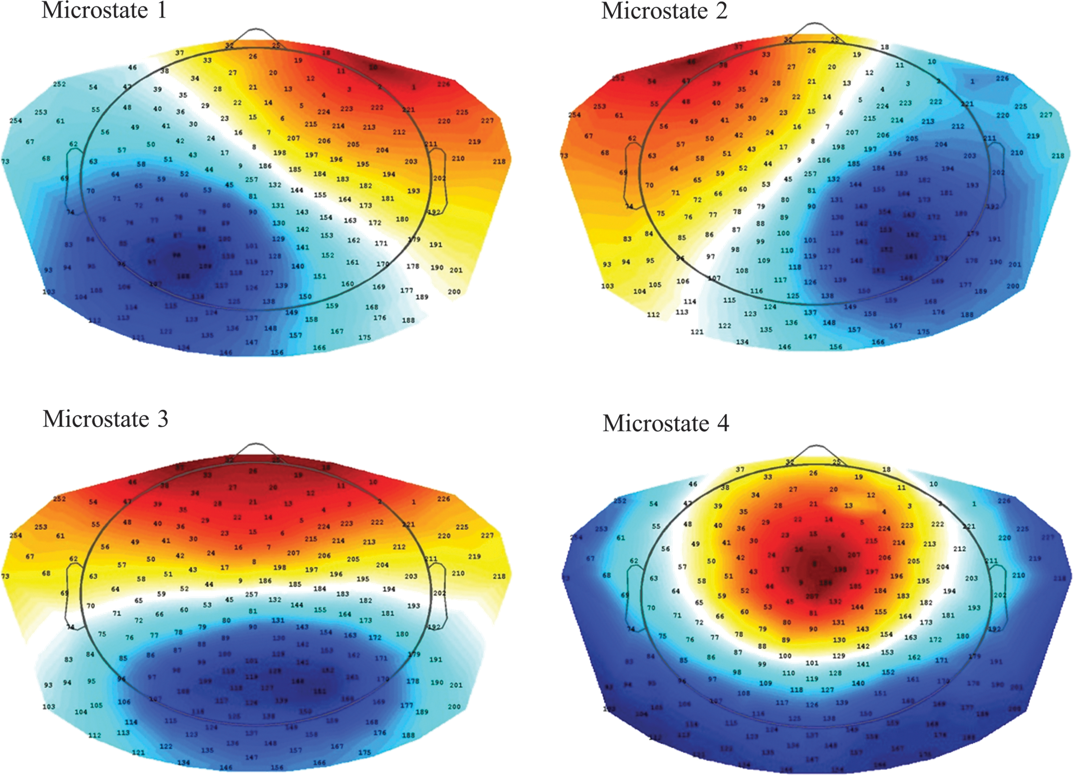
Four microstates derived from K-means clustering on baseline electroencephalography using squared correlation as distance measure. Note also that the polarity (color code) is chosen arbitrarily, as microstates are independent from polarity switches that might occur within topographies.

Functional connectivity

For measuring connectivity, the PLI was selected, as this index is known to be little affected by the effect of volume conduction compared to other classical connectivity measures such as synchronization likelihood, phase coherence, or envelope correlation (Stam and van Dijk, 2002). PLI measures were first calculated in a standard approach. Data were filtered using a Butterworth filter to four predefined frequency bands (theta: 4–8 Hz, alpha1: 8–10 Hz, alpha2: 10–13 Hz, and beta: 13–30 Hz). Phase estimation was archived using a Hilbert transformation. The phase difference distribution was obtained from a time series (t1−tk) of phase differences (Δφ) between two signals and the asymmetry of the phase difference distribution was calculated as described by Stam et al. (2007). \documentclass{aastex}\usepackage{amsbsy}\usepackage{amsfonts}\usepackage{amssymb}\usepackage{bm}\usepackage{mathrsfs}\usepackage{pifont}\usepackage{stmaryrd}\usepackage{textcomp}\usepackage{portland, xspace}\usepackage{amsmath, amsxtra}\pagestyle{empty}\DeclareMathSizes{10}{9}{7}{6}\begin{document} \begin{align*}PLI = \frac { 1 } { k } \left| { \mathop \sum \limits_ { t = 1 } ^k sign \left[ { \sin \left( { { \Delta } \phi \left( t \right) } \right) } \right] } \right|\end{align*} \end{document}

(where k = number of samples, Δφ = phase differences between two channels)

PLI was calculated using four epochs of 4 sec and averaging the resulting matrix into one matrix per subject and frequency band, as described previously (Hardmeier et al., 2014).

Functional connectivity within microstate-segmented PLI

In the second approach, PLI was calculated within microstate segments. To this aim, the Hilbert transformation was applied to the full-length EEG using a sliding window of 4 sec with a 50% Hanning window. For every microstate class, four stitched periods of each 4000-phase difference ( = 4 sec) were then extracted, using the time frames indicated by the microstate label vector and automated routines to detect microstates with lowest number of bad channels and avoiding periods were inverse Hanning windows were applied. The number of four epochs per microstate, subject, and frequency band was selected, as this minimal amount of epochs per microstate was available in almost all EEG, given the recording time of EEG data. Like in the standard approach, the four resulting matrices (one per frequency band) were averaged per subject, for each microstate class separately.

Graph measures

Graph measures were calculated according to the formulas in Table 1: average clustering coefficient (Cw), average shortest path length (Lw), degree diversity (Kw), and degree correlation (Rw) were selected. Cw stands for the amount of local connectivity, and Lw for the optimization of distant connectivities. The lower the Lw and the higher the Cw, the more information flow is optimized toward a small world network. Kw represents the distribution of degrees; a high value stands for a network with only a few highly connected nodes, also called hubs. Degree correlation represents a similar characteristic and is high when nodes with similar degrees are connected. Moreover, graph measures derived from a minimum spanning tree (MST) analysis were added. MST analysis allows to identify the “main roads” of a network, reduces the network to a fixed number of connections (number of nodes minus one), and simplifies statistical analysis and comparison of different networks.

Table 1.

Graph Measures as Calculated for Each Subject

Name		Formula	References
Average clustering coefficient	Cw	\documentclass{aastex}\usepackage{amsbsy}\usepackage{amsfonts}\usepackage{amssymb}\usepackage{bm}\usepackage{mathrsfs}\usepackage{pifont}\usepackage{stmaryrd}\usepackage{textcomp}\usepackage{portland, xspace}\usepackage{amsmath, amsxtra}\pagestyle{empty}\DeclareMathSizes{10}{9}{7}{6}\begin{document}$Cw = mean \left( C \right)$ \end{document}	Stam et al. (2009)
		\documentclass{aastex}\usepackage{amsbsy}\usepackage{amsfonts}\usepackage{amssymb}\usepackage{bm}\usepackage{mathrsfs}\usepackage{pifont}\usepackage{stmaryrd}\usepackage{textcomp}\usepackage{portland, xspace}\usepackage{amsmath, amsxtra}\pagestyle{empty}\DeclareMathSizes{10}{9}{7}{6}\begin{document}$ { C_i } = { \frac { \mathop \sum \nolimits_ { k \ne i } \mathop \sum \nolimits_ { \begin{matrix} { l \ne i } \\ { l \ne k } \\ \end{matrix} } { W_ { ik } } { W_ { il } } { W_ { kl } } } { \mathop \sum \nolimits_ { k \ne i } \mathop \sum \nolimits_ { \begin{matrix} { l \ne i } \\ { l \ne k } \\ \end{matrix} }{ W_ { ik } } { W_ { il } } } } $ \end{document}
Normalized clustering coefficient	Gamma	Cw/Cr (Cr = average of 50 randomized input matrices)	Spoormaker et al. (2010)
Average path length	Lw	\documentclass{aastex}\usepackage{amsbsy}\usepackage{amsfonts}\usepackage{amssymb}\usepackage{bm}\usepackage{mathrsfs}\usepackage{pifont}\usepackage{stmaryrd}\usepackage{textcomp}\usepackage{portland, xspace}\usepackage{amsmath, amsxtra}\pagestyle{empty}\DeclareMathSizes{10}{9}{7}{6}\begin{document}$L = {1 / {weight}}$ \end{document}	Stam et al. (2009)
		\documentclass{aastex}\usepackage{amsbsy}\usepackage{amsfonts}\usepackage{amssymb}\usepackage{bm}\usepackage{mathrsfs}\usepackage{pifont}\usepackage{stmaryrd}\usepackage{textcomp}\usepackage{portland, xspace}\usepackage{amsmath, amsxtra}\pagestyle{empty}\DeclareMathSizes{10}{9}{7}{6}\begin{document}$L = \infty\ ( if \ weight = 0 )$ \end{document}
		\documentclass{aastex}\usepackage{amsbsy}\usepackage{amsfonts}\usepackage{amssymb}\usepackage{bm}\usepackage{mathrsfs}\usepackage{pifont}\usepackage{stmaryrd}\usepackage{textcomp}\usepackage{portland, xspace}\usepackage{amsmath, amsxtra}\pagestyle{empty}\DeclareMathSizes{10}{9}{7}{6}\begin{document}$Lw = \frac { 1 } { { \frac { 1 } { { N \left( { N - 1 } \right)} } ^ * \mathop \sum \nolimits_ { i = 1 } ^N \mathop \sum \nolimits_ { j \ne i } ^N ( 1 / { L_ { ij } } ) } } $ \end{document}
Normalized average path length	Lambda	Lw/Lr (Lr = average of 50 randomized matrices)	Spoormaker et al. (2010)
Degree correlation	Rw	Rw = Pearson correlation of degrees of pairs of neighbors	Newman (2003)
Degree diversity	Kw	\documentclass{aastex}\usepackage{amsbsy}\usepackage{amsfonts}\usepackage{amssymb}\usepackage{bm}\usepackage{mathrsfs}\usepackage{pifont}\usepackage{stmaryrd}\usepackage{textcomp}\usepackage{portland, xspace}\usepackage{amsmath, amsxtra}\pagestyle{empty}\DeclareMathSizes{10}{9}{7}{6}\begin{document}$Kw = \frac { { ( degree^ { 2 } } ) } { ( { degree } ) } $ \end{document}	Stam and van Straaten (2012b)
MST	MST	Kruskal's algorithm	Boersma et al. (2013)
MST betweenness centrality	MSTBC	Betweenness centrality = fraction of all shortest paths that pass through a particular vertex, maximal value of all vertices	Wang et al. (2008)
MST degree correlation	MSTR	See Rw
MST degree diversity	MSTKappa	See Kw
MST diameter	MSTDiam	Longest shortest path of MST-graph
MST leaf nodes	MSTLeaf	Number of nodes with degree of 1

MST, minimum spanning tree.

Statistics

For statistical analysis, the 214 electrodes were grouped into 22 regions across the scalp (11 regions per hemisphere), excluding electrodes in the midline, neck, and face (Hardmeier et al., 2014); for connectivities, the average was taken of all connectivities connecting two regions.

Graphs of the different microstates and frequency bands were compared using a Pearson correlation analysis (subjectwise). Cross-sectional intersubject variability was expressed as the coefficient of variation (CoV) calculated as the ratio between the standard deviation and the mean of the PLI/msPLI. For TRT reliability over the three time points (i.e., across annual EEG recordings), intraclass correlation coefficients (ICC) were calculated (Efron, 1979). A bootstrapping procedure with 10,000 permutations was performed to estimate the 95% confidence interval (95% CI) for both indices and correcting artifacts of ICC. In accordance with previous studies, reliability was categorized as “excellent” if ICC >0.75, as “good” if ICC: 0.60–0.75, as “fair” if ICC: 0.40–0.60, and as “poor” if ICC <0.40 (Deuker et al., 2009; Jin et al., 2011; Wang et al., 2011).

The Code of TAPEEG, including the combined analysis of microstates and connectivity, is freely available under “https://sites.google.com/site/tapeeg”.

Results

Preprocessing

The automated analysis of quality criteria rejected at least one recording in the EEG of six subjects, resulting in a remaining total of 34 subjects for further analysis.

Microstate analysis revealed an optimal clustering number of four microstates (Fig. 1), consistent with previous literature (Khanna et al., 2015; Koenig, 2002). Global explained variance for the result with four microstates was 0.67. Median durations and lower–upper quartiles of single microstates are given in Supplementary Table S1 (Supplementary Data are available online at www.liebertpub.com/brain).

Connectivity analysis

Results are given in Figure 2 and Tables 2, 3.

FIG. 2.

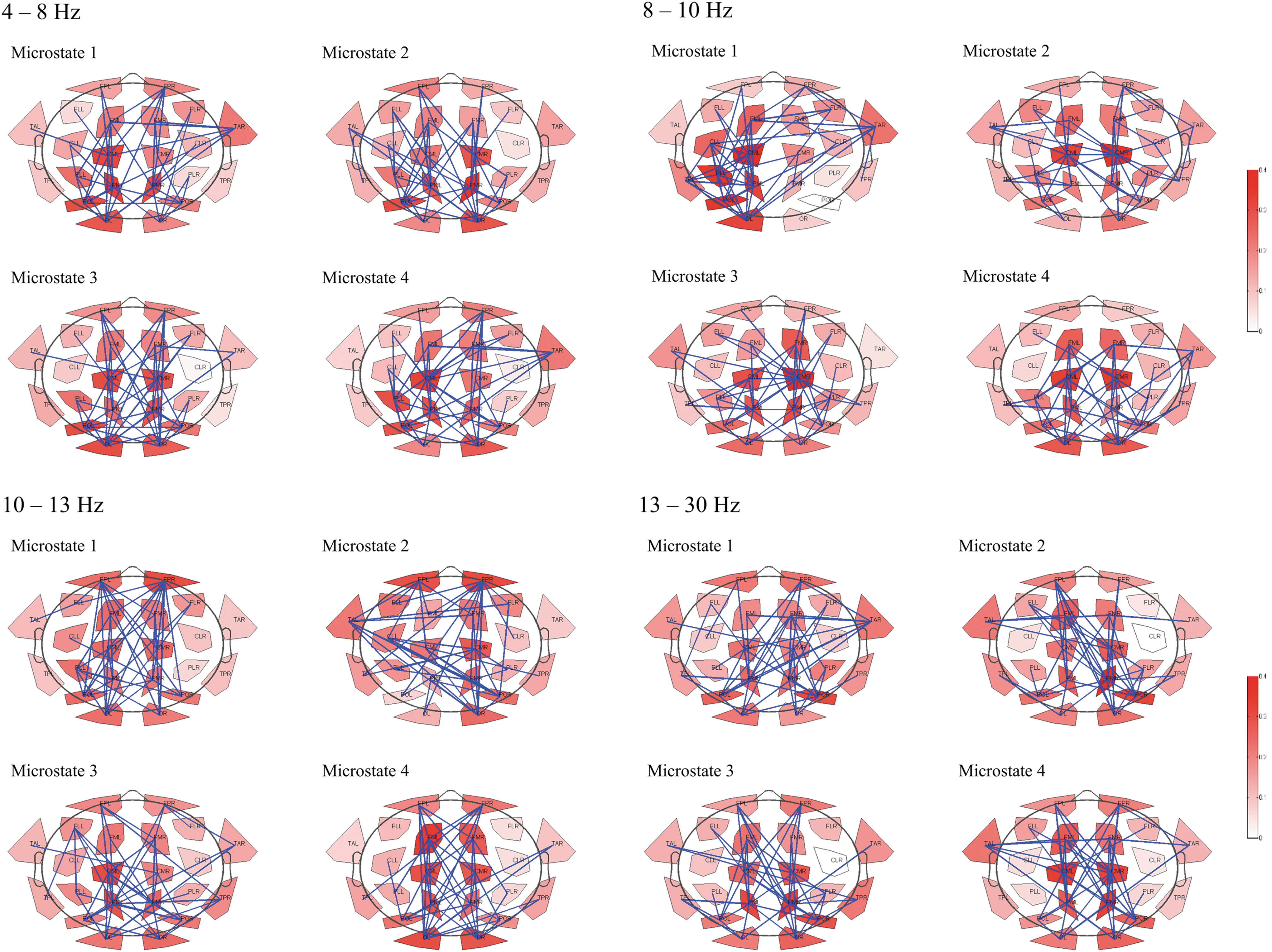
Connectomes of single microstates averaged across all participants. Connectomes were reduced to 22 nodes. Only the 20% strongest links are plotted. Nodal degrees are shown in red.

Table 2.

Intraclass Correlation, Median Values of All Links

ICC	4–8 Hz	8–10 Hz	10–13 Hz	13–30 Hz
No microstates	0.47 (0.18–0.73)	0.61 (0.43–0.79)	0.58 (0.41–0.75)	0.42 (0.2–0.63)
Microstate 1	0.58 (0.22–0.81)	0.66 (0.47–0.84)	0.7 (0.55–0.83)	0.27 (0.054–0.5)
Microstate 2	0.69 (0.18–0.89)	0.63 (0.44–0.8)	0.54 (0.34–0.73)	0.18 (−0.02–0.42)
Microstate 3	0.74 (0.47–0.88)	0.77 (0.6–0.89)	0.77 (0.66–0.86)	0.48 (0.25–0.71)
Microstate 4	0.79 (0.55–0.9)	0.7 (0.49–0.86)	0.71 (0.56–0.83)	0.31 (0.089–0.56)

Median values were selected, as resulting ICC values were not normally distributed; parenthesis: lower and upper quartile of bootstrapping analysis; bold: “excellent” TRT.

ICC, intraclass correlation coefficients.

Table 3.

Coefficient of Variation, Median Values of All Links, and Time Points

CoV	4–8 Hz	8–10 Hz	10–13 Hz	13–30 Hz
No microstates	0.21 (0.17–0.26)	0.28 (0.24–0.34)	0.32 (0.28–0.4)	0.21 (0.18–0.26)
Microstate 1	0.32 (0.26–0.42)	0.43 (0.37–0.52)	0.51 (0.44–0.62)	0.24 (0.21–0.3)
Microstate 2	0.44 (0.33–0.61)	0.43 (0.38–0.53)	0.49 (0.41–0.6)	0.25 (0.21–0.31)
Microstate 3	0.31 (0.24–0.43)	0.42 (0.37–0.51)	0.45 (0.41–0.53)	0.21 (0.18–0.26)
Microstate 4	0.48 (0.38–0.61)	0.49 (0.44–0.59)	0.51 (0.45–0.61)	0.25 (0.21–0.32)

Parenthesis: lower and upper quartile of bootstrapping analysis; bold: “excellent” CoV.

CoV, coefficient of variation.

For visual comparison of the different network graphs derived from averaging, the four connectomes per frequency band and microstate were transformed to binary graphs, setting only the 20% strongest links to one, averaged across subjects, and again thresholded at 20% strongest connections (Fig. 2). Pearson correlation of the graphs in the different frequency bands and microstates revealed higher correlations within each frequency band across different microstates than between the different frequency bands for the same microstate (Fig. 3). The correlations were significant for the microstates in the alpha1, alpha2, and beta band. No significant correlations between the graphs of different frequency bands were found.

FIG. 3.

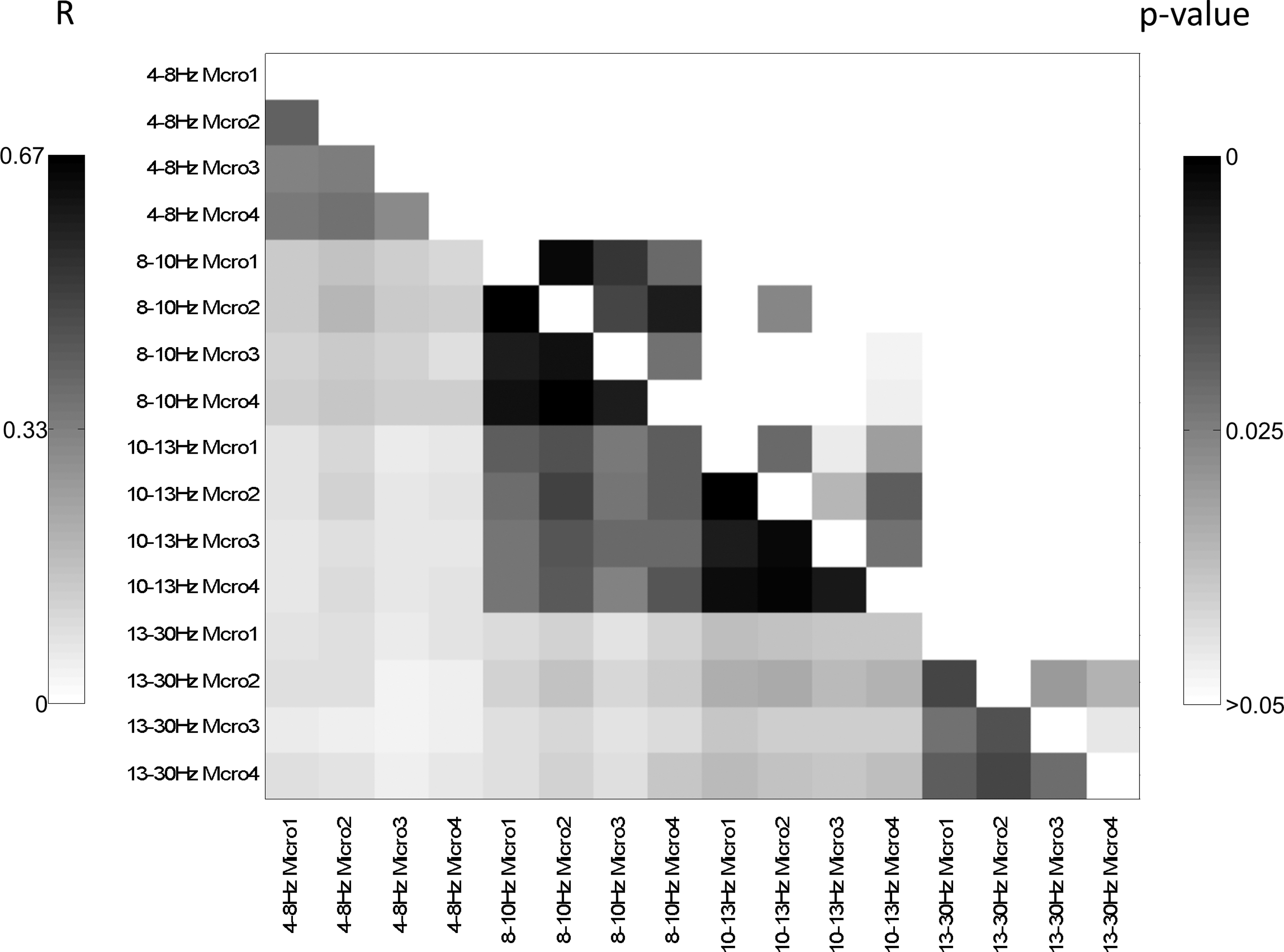
Connectomes were reduced to 22 nodes and Pearson correlations were calculated subject wise. Mean correlation values are shown in the lower, mean p-values in the upper triangle. In the upper triangle, only p-values ≤0.05 are shown, in the lower triangle, all correlation values are shown regardless the significance.

After reduction of the connectivity results to 22 regions, the regional-link analysis showed “excellent” TRT reliability across the three time points T0, T1, and T2 (median ICC >0.75) for theta connectivity in microstate 4, for alpha1 and alpha2 connectivity in microstate 3, and “good” TRT reliability (median ICC >0.6) for other theta, alpha1, and alpha2 microstate connectivities (Table 2). The ICC results of the regional-link analysis without microstates were distinctly lower (Table 2 and Supplementary Fig. S1). CoV results are provided in Table 3.

Graph analysis

Results of graph measures analysis are listed in Table 4. In the theta, alpha1, and alpha2 band, “good” to “excellent” TRT reliability is seen for Cw, Lw, and Kw, but not for gamma, lambda, Rw, or results in the beta band and graph measures derived from MST analysis (Supplementary Table S2).

Table 4.

ICC for Graph Measures in Theta, Alpha1, Alpha2, and Beta Frequency Band and for Different Microstates

ICC	4–8 Hz	8–10 Hz	10–13 Hz	13–30 Hz
No microstates
Weight	0.69 (0.04–0.93)	0.65 (−0.1–0.81)	0.29 (−0.13–0.6)	0.64 (0.14–0.89)
Average clustering coefficient	0.7 (0.04–0.92)	0.43 (−0.15–0.78)	0.43 (−0.15–0.78)	0.64 (0.14–0.89)
Average shortest path	0.42 (−0.04–0.83)	0.25 (−0.15–0.56)	0.25 (−0.15–0.56)	0.62 (0.13–0.87)
Degree correlation	0.64 (0.01–0.92)	0.23 (−0.3–0.65)	0.76 (0.35–0.91)	0.44 (0.02–0.75)
Degree diversity	0.68 (0.28–0.85)	0.68 (0.28–0.85)	0.76 (0.34–0.91)	0.64 (0.14–0.89)
Microstate 1
Weight	0.79 (0.52–0.9)	0.78 (0.63–0.89)	0.79 (0.63–0.9)	0.34 (0.16–0.57)
Average clustering coefficient	0.81 (0.49–0.91)	0.79 (0.64–0.89)	0.79 (0.63–0.89)	0.36 (0.19–0.62)
Average shortest path	0.67 (0.33–0.86)	0.75 (0.61–0.86)	0.8 (0.7–0.88)	0.26 (0.05–0.48)
Degree correlation	0.07 (−0.11–0.29)	0.34 (0.16–0.54)	0.21 (0.01–0.5)	0.14 (−0.01–0.39)
Degree diversity	0.8 (0.5–0.91)	0.78 (0.64–0.89)	0.79 (0.63–0.9)	0.35 (0.18–0.6)
Microstate 2
Weight	0.79 (0.41–0.88)	0.79 (0.66–0.88)	0.63 (0.5–0.76)	0.22 (0.08–0.36)
Average clustering coefficient	0.8 (0.42–0.88)	0.79 (0.66–0.88)	0.64 (0.5–0.76)	0.27 (0.13–0.43)
Average shortest path	0.62 (0.29–0.84)	0.76 (0.64–0.86)	0.68 (0.49–0.78)	0.27 (0.12–0.46)
Degree correlation	0.06 (−0.11–0.27)	0.03 (−0.15–0.23)	0.05 (−0.1–0.18)	0.15 (−0.02–0.36)
Degree diversity	0.8 (0.42–0.88)	0.78 (0.66–0.88)	0.64 (0.5–0.76)	0.24 (0.1–0.39)
Microstate 3
Weight	0.8 (0.5–0.93)	0.83 (0.72–0.93)	0.76 (0.67–0.85)	0.42 (0.2–0.58)
Average clustering coefficient	0.81 (0.52–0.93)	0.83 (0.72–0.92)	0.77 (0.69–0.85)	0.43 (0.22–0.59)
Average shortest path	0.67 (0.45–0.85)	0.79 (0.7–0.88)	0.81 (0.72–0.89)	0.43 (0.23–0.64)
Degree correlation	0.29 (0.05–0.61)	0.19 (0–0.4)	0.07 (−0.13–0.27)	−0.07 (−0.22–0.09)
Degree diversity	0.81 (0.51–0.94)	0.83 (0.72–0.92)	0.77 (0.68–0.85)	0.42 (0.2–0.59)
Microstate 4
Weight	0.87 (0.75–0.92)	0.78 (0.56–0.91)	0.78 (0.69–0.85)	0.45 (0.28–0.64)
Average clustering coefficient	0.89 (0.75–0.93)	0.78 (0.55–0.9)	0.79 (0.7–0.87)	0.49 (0.32–0.71)
Average shortest path	0.74 (0.54–0.87)	0.73 (0.6–0.84)	0.74 (0.62–0.84)	0.55 (0.36–0.73)
Degree correlation	−0.05 (−0.22–0.1)	0.23 (0.08–0.38)	0.01 (−0.13–0.24)	−0.03 (−0.16–0.14)
Degree diversity	0.88 (0.74–0.92)	0.78 (0.56–0.9)	0.79 (0.7–0.86)	0.47 (0.3–0.68)

Parenthesis: lower and upper quartile of bootstrapping analysis; bold: “excellent” TRT.

Discussion

Microstate-segmented PLI (msPLI) revealed a significantly higher TRT reliability over a 2-year follow-up period for single-link and regional-link analysis compared to standard PLI analysis. A possible explanation is that during each microstate, EEG data have a higher stationarity than without such segmentation. Microstates are defined by stable topographies of electrical brain activity with a mean duration of around 100 ms, explained by synchronized oscillations (Koenig et al., 2005). According to Koenig, two physical models of the microstates have been proposed. In a first model, a single strong electrical source causes the corresponding microstate by volume conduction. In a second model, multiple active electrical sources are operating in a phase-locked, zero-lag mode. By applying inverse solution techniques, each microstate can geometrically be reduced to the activity of circumscribed regions deeper in the brain (Pascual-Marqui et al., 2014). These regions are too extended to represent single electrical sources, and the concept of a deeper located group of sources with phase-locked, zero-lag synchronization is more likely. As a consequence, the part of electrical activity explaining the microstate measured at a single electrode would not necessarily be generated in direct proximity of the electrode. Therefore, brain activity as measured at a single electrode is composed of signals from many simultaneously active electrical sources, among them those defining the microstate. As the activity of more superficially located electrical sources is not as equally propagated to all electrodes as the activity of deeper electrical sources, the more superficially located activity is more likely to produce signals with phase shifts between single electrodes. By calculating the PLI (Stam et al., 2007), only the consistency of these phase shifts is evaluated, excluding information of oscillations without phase shifts (nonlagged oscillations).

In this study, PLI was calculated for the four different microstates separately by segmenting the phase information according to the initial microstate segmentation. The higher TRT reliability compared to classical PLI analysis is an argument for connectivity being influenced by microstates and for the concept of subnetworks depicted in single microstates (Stam and van Straaten, 2012b): the corresponding subnetwork shows increased activity during a single microstate when compared with other subnetworks, leading to a better signal-to-noise ratio for a reliable detection of a true phase consistency and resulting in the identification of links with stronger connectivity values than in an analysis without microstates. The larger range of connectivity values may explain the higher CoV values in msPLI compared with classical PLI evaluation. TRT reliability in regional-link compared to single-link analysis is distinctly higher. This may be explained by the individual placements of the high-resolution EEG nets for every single investigation, leading to small shifts of single electrodes from one to the next recording. Thinking about a maximal shift of one electrode, we decided to average the electrodes to 22 groups. The number of 22 groups is a compromise between avoiding too much obvious volume conduction effects while still representing some functional regions, even in some more detail than in Berendse and Stam (2007) using 10 regions.

Derived graph measures from msPLI connectivity results are also showing improved reliability over time compared with the analysis without microstates. Interestingly, “good” to “excellent” reliability was found for the average clustering coefficient (Cw), average shortest path length (Lw), and degree diversity, but not for normalized Cw and Lw, degree correlation (also called assortativity), or results of the MST analysis. In comparison with single-link analysis, graph measures showed lower reliability. However, these results are not easily comparable, as for single-link analysis, we reduced the number of links using a mapping to 22 regions, whereas graph analysis was performed on the full matrices with 214 nodes. By not reducing the number of nodes, the signal-to-noise ratio and consecutively the TRT reliability may be lower. A graph analysis on data with a reduced number of links is not included, as interpretation of graph results derived from connectomes with a low number of nodes is difficult. Lower connectivity values are hardly distinguishable from noise and only averaging of a larger number of matrices in the same subject improves the signal-to-noise ratio. This fact may explain the very low reliability for MST-derived graph measures. MST analysis depends partially on reliable lower connectivity strengths, as in MST, every node has at least one connection (degree ≥1). In the present study, only four matrices per subject and microstate could be included, due to the maximal available amount of recorded and preprocessed data (12-min continuous resting-state data per subject). Recording longer periods of continuous resting-state EEG may be increasingly contaminated with instable vigilance. For this reason, msPLI analysis will be limited to an analysis with a reduced set of matrices per subject and microstate, and it will be of reduced value for analyses that significantly depend on reliable lower connectivity strengths such as MST analysis.

Some earlier studies also reported on TRT reliability of connectivity and graph measures. For eyes closed resting-state analysis, Jin and colleagues reported fair to moderate TRT reliability for different nodal centrality measures at a test–retest interval of 2 weeks using magnetoencephalography (MEG) and mutual information as connectivity measure. TRT reliability was partly higher in the eyes-open compared to the eyes-closed resting state, and much lower in the gamma band (Jin et al., 2011). Deuker et al. (2009) recorded eyes-closed resting-state MEG data at a test–retest interval of 4–6 weeks and reported an excellent ICC for Lw and “efficiency” ( = 1/Lw) and a good ICC for Kw in a broader alpha band (7.8–15.6 Hz). However, these studies are not directly comparable to the present study as EEG and MEG are picking up signals from different sources (gyri vs. sulci) (Malmivuo, 2012) and mutual information reflects other aspects of connectivity between two regions as phase-derived graph measures, including the PLI (David et al., 2004).

The present observation of significantly high correlations between the connectomes of the four different microstates in every frequency band is another argument in favor of the assumption that microstates reflect activity of different subnetworks in a global network (Stam and van Straaten, 2012b; Van De Ville et al., 2010). This assumption is in line with previous work, describing all microstates as a part of the default mode network in resting state (Pascual-Marqui et al., 2014), or, alternatively, that four distinct networks are continuously active with changing intensity (Britz et al., 2010; Musso et al., 2010). Differentiating between the two possibilities is not possible based on the results of this study.

A synthesis of both possibilities might be the concept of the brain as one large network with dedicated subnetworks for different tasks, which are simultaneously active and interdependent to a certain degree.

However, thinking about the brain as one large network with dedicated subnetworks for different tasks, it is more convincing to believe in the approach where all simultaneously active networks are at a certain degree linked and dependent. The observation of stronger ICC results in the alpha1 and alpha2 band is most probably explained by the paradigm selected for the study. EEG was recorded in resting state with eyes closed, leading to most prominent power in the alpha band. Since PLI strength is positively correlated with power results (unpublished data of our group), the increased ICC values in alpha1 and alpha2 bands are likely the result of the higher PLI values in these bands. The same relationship may also explain the reduced ICC values in the beta band, as the power in the beta band is lowest, reducing the signal-to-noise ratio for the PLI calculation. In addition, the fact of averaging only four matrices per microstate leads to difficult interpretation of results in the beta band.

Validation studies combining microstates and connectivity analysis in patient cohorts are warranted.

Conclusion

The combination of microstates and phase-derived connectivity measures such as PLI improves reliability of single-link, regional-link, and graph analysis.

Footnotes

Acknowledgments

We thank the participating subjects. The financial support of the Swiss National Science Foundation (Grant Nos.: 33CM30_140338, 33CM30_124115; 326030-128775/1), Synapsis/Parrotia Foundation, Novartis Research Foundation, Freiwillige Akademische Gesellschaft Basel, Mach-Gaensslen Foundation, and Swiss Multiple Sclerosis Society is gratefully acknowledged.

Author Disclosure Statement

No competing financial interests exist.

References

Bassett

, Meyer-Lindenberg

, Achard

, Duke

, Bullmore

. 2006. Adaptive reconfiguration of fractal small-world human brain functional networks. Proc Natl Acad Sci, 103:19518–19523.

Berendse

, Stam

. 2007. Stage-dependent patterns of disturbed neural synchrony in Parkinson's disease. Parkinsonism Relat Disord, 13 (Suppl 3):S440–S445.

Boersma

, Smit

DJA

, Boomsma

, De Geus

EJC

, Delemarre-van de Waal

, Stam

. 2013. Growing trees in child brains: graph theoretical analysis of electroencephalography-derived minimum spanning tree in 5- and 7-year-old children reflects brain maturation. Brain Connect, 3:50–60.

Britz

, Van De Ville

, Michel

. 2010. BOLD correlates of EEG topography reveal rapid resting-state network dynamics. NeuroImage, 52:1162–1170.

Bullmore

, Sporns

. 2012. The economy of brain network organization. Nat Rev Neurosci, 13:336–349.

David

, Cosmelli

, Friston

. 2004. Evaluation of different measures of functional connectivity using a neural mass model. NeuroImage, 21:659–673.

Deuker

, Bullmore

, Smith

, Christensen

, Nathan

, Rockstroh

, et al. 2009. Reproducibility of graph metrics of human brain functional networks. Neuroimage, 47:1460–1468.

Efron

. 1979. Bootstrap methods: another look at the jackknife. Ann Stat, 7:1–26.

Fell

, Axmacher

. 2011. The role of phase synchronization in memory processes. Nat Rev Neurosci, 12:105–118.

10.

Hardmeier

, Hatz

, Bousleiman

, Schindler

, Stam

, Fuhr

. 2014. Reproducibility of functional connectivity and graph measures based on the phase lag index (PLI) and weighted phase lag index (wPLI) derived from high resolution EEG. PLoS One, 9:e108648.

11.

Hatz

, Hardmeier

, Bousleiman

, Rüegg

, Schindler

, Fuhr

. 2015. Reliability of fully automated versus visually controlled pre- and post-processing of resting-state EEG. Clin Neurophysiol, 126:268–274.

12.

Jin

S-H

, Seol

, Kim

, Chung

. 2011. How reliable are the functional connectivity networks of MEG in resting states?. J Neurophysiol, 106:2888–2995.

13.

Khanna

, Pascual-Leone

, Farzan

. 2014. Reliability of resting-state microstate features in electroencephalography. PLoS One, 9:e114163.

14.

Khanna

, Pascual-Leone

, Michel

, Farzan

. 2015. Microstates in resting-state EEG: current status and future directions. Neurosci Biobehav Rev, 49C:105–113.

15.

Koenig

. 2002. Millisecond by millisecond, year by year: normative EEG microstates and developmental stages. NeuroImage, 16:41–48.

16.

Koenig

, Studer

, Hubl

, Melie

, Strik

. 2005. Brain connectivity at different time-scales measured with EEG. Philos Trans R Soc B Biol Sci, 360:1015–1024.

17.

Krzanowski

, Lai

. 1988. A criterion for determining the number of groups in a data set using sum-of-squares clustering. Biometrics, 44:23–34.

18.

Malmivuo

. 2012. Comparison of the properties of EEG and MEG in detecting the electric activity of the brain. Brain Topogr, 25:1–19.

19.

Michel

, Lehmann

. 1993. Single doses of piracetam affect 42-channel event-related potential microstate maps in a cognitive paradigm. Neuropsychobiology, 28:212–221.

20.

Murray

, Brunet

, Michel

. 2008. Topographic ERP analyses: a step-by-step tutorial review. Brain Topogr, 20:249–264.

21.

Musso

, Brinkmeyer

, Mobascher

, Warbrick

, Winterer

. 2010. Spontaneous brain activity and EEG microstates. A novel EEG/fMRI analysis approach to explore resting-state networks. NeuroImage, 52:1149–1161.

22.

Nevado

, Hadjipapas

, Kinsey

, Moratti

, Barnes

, Holliday

, et al. 2012. Estimation of functional connectivity from electromagnetic signals and the amount of empirical data required. Neurosci Lett, 513:57–61.

23.

Newman

MEJ

. 2003. Mixing patterns in networks. Phys Rev E Stat Nonlin Soft Matter Phys, 67:026126.

24.

Pascual-Marqui

, Lehmann

, Faber

, Milz

, Kochi

, Yoshimura

, et al. 2014. The resting microstate networks (RMN): cortical distributions, dynamics, and frequency specific information flow. arXiv: 1411.1949v2

25.

Pascual-Marqui

, Michel

, Lehmann

. 1995. Segmentation of brain electrical activity into microstates: model estimation and validation. Biomed Eng IEEE Trans On, 42:658–665.

26.

Perrin

, Pernier

, Bertrand

, Echallier

. 1989. Spherical splines for scalp potential and current density mapping. Electroencephalogr Clin Neurophysiol, 72:184–187.

27.

Spoormaker

, Schroter

, Gleiser

, Andrade

, Dresler

, Wehrle

, et al. 2010. Development of a large-scale functional brain network during human non-rapid eye movement sleep. J Neurosci, 30:11379–11387.

28.

Stam

, De Haan

, Daffertshofer

, Jones

, Manshanden

, van Cappellen van Walsum

, et al. 2009. Graph theoretical analysis of magnetoencephalographic functional connectivity in Alzheimer's disease. Brain, 132:213.

29.

Stam

, Nolte

, Daffertshofer

. 2007. Phase lag index: assessment of functional connectivity from multi channel EEG and MEG with diminished bias from common sources. Hum Brain Mapp, 28:1178–1193.

30.

Stam

, van Dijk

. 2002. Synchronization likelihood: an unbiased measure of generalized synchronization in multivariate data sets. Phys Nonlinear Phenom, 163:236–251.

31.

Stam

, van Straaten

ECW

. 2012a. Go with the flow: use of a directed phase lag index (dPLI) to characterize patterns of phase relations in a large-scale model of brain dynamics. NeuroImage, 62:1415–1428.

32.

Stam

, van Straaten

ECW

. 2012b. The organization of physiological brain networks. Clin Neurophysiol, 123:1067–1087.

33.

Van De Ville

, Britz

, Michel

. 2010. EEG microstate sequences in healthy humans at rest reveal scale-free dynamics. Proc Natl Acad Sci, 107:18179–18184.

34.

Wang

, Hernandez

, Van Mieghem

. 2008. Betweenness centrality in a weighted network. Phys Rev E Stat Nonlin Soft Matter Phys, 77:046105.

35.

Wang

S-J

, Hilgetag

, Zhou

. 2011. Sustained activity in hierarchical modular neural networks: self-organized criticality and oscillations. Front Comput Neurosci, 5:30.

Supplementary Material

Please find the following supplemental material available below.

For Open Access articles published under a Creative Commons License, all supplemental material carries the same license as the article it is associated with.

For non-Open Access articles published, all supplemental material carries a non-exclusive license, and permission requests for re-use of supplemental material or any part of supplemental material shall be sent directly to the copyright owner as specified in the copyright notice associated with the article.

0.00 MB

0.06 MB

0.01 MB

0.02 MB