Graph Measures of Node Strength for Characterizing Preictal Synchrony in Partial Epilepsy

Abstract

The reference electrophysiological pattern at seizure onset is the “rapid discharge,” as visible on intracerebral electroencephalography (EEG). This discharge typically corresponds to a decrease of synchrony across brain areas. In contrast, the preictal period can exhibit patterns of increased synchrony, which can be quantified by network measures. Our objective was to compare preictal synchrony with a quantification of the rapid discharge as provided by the epileptogenicity index (EI). We investigated 24 seizures from 12 patients recorded by stereotaxic EEG (SEEG). Seizures were classified visually as containing preictal synchrony or not. We computed pairwise nonlinear correlation (h ²) across channels in the 8 sec preceding the rapid discharge. The sum of ingoing and outgoing links (IN and OUT node strength), as well as the sum of all links (total strength, TOT) were computed for each region. We tested several filtering schemes, and quantified the capacity of each strength measure to serve as a detector of regions with high EI values using a receiver operating characteristic (ROC) analysis. We found that the best correspondence between node strength and EI was obtained for the OUT and TOT measures, for signals filtered in the 15–40 Hz band—that is, for the band corresponding to the spiky part of epileptic discharges. In agreement with these results, we also found that the ROC results were improved when considering only seizures with visible synchronous patterns in the preictal period. Our results suggest that measuring strength of preictal connectivity graphs can bring useful clinical information on the epileptogenic zone.

Introduction

Seizures are classically considered as the hallmark of epilepsy. Their onset can either be focal, with subsequent propagation to other brain areas, or be distributed from the start over large networks (Bartolomei et al., 2013; Stefan and Lopes da Silva, 2013). The electrophysiological pattern usually taken as a reference of the onset of seizure is the “rapid discharge,” as visible on intracerebral electroencephalography (EEG). This discharge consists in a flattening of signals, corresponding to an increase of the high frequency content and a decrease of low frequencies. Recently, several methods have been proposed to quantify the spatiotemporal distribution of rapid discharge (Andrzejak et al., 2014). Among them, the epileptogenicity index (EI) has been introduced to quantify the epileptogenic nature of each recording site based on both frequency content and delay with respect to seizure start (Bartolomei et al., 2008). Thus, the EI permits to track the involvement of the different brain structures within the seizure onset network.

The h ² nonlinear correlation index allows characterizing the degree of synchronization across different brain regions (Lopes da Silva et al., 1989; Wendling and Bartolomei, 2001a). Even though epilepsy is a disease involving hypersynchrony, the initial part of the rapid discharge has been shown—somehow paradoxically—to correspond to a decrease of synchrony across brain areas (Wendling et al., 2003). Nevertheless, synchrony is observed in later part of the seizure, as well as in the interictal state—in particular, in the period directly preceding the seizure, the preictal period (Bartolomei et al., 2004). The question then arises of the relationship between patterns of preictal synchrony—potentially leading to the rapid discharge—and the regions involved in the start of the rapid discharge. In other words, one may ask whether the preictal brain dynamics evolve progressively into a seizure pattern (Schwartz et al., 2011).

Clinically, a better understanding of the preictal synchrony patterns could improve the definition of the regions to be removed for abolishing seizures. At a more fundamental level, it could give insights on the mechanisms occurring at the transition between the interictal and ictal state.

Synchrony measures can be used to track the evolution of the coupling between brain areas over time. However, these spatiotemporal patterns become easily intractable and complex as the size of the network (i.e., the number of channels) increases. Graph theory provides measures that summarize such information into useful metrics, especially in the case of ictal activities (Ponten et al., 2007). Of particular interest for epilepsy are the in-degrees and out-degrees, which measure the number of input or output links from a given region. This permits in turn to define leading regions, that is, “drivers,” that are potentially more epileptogenic (van Mierlo et al., 2013).

The objective of our study was, therefore, to quantify the patterns of synchrony occurring before the start of the rapid discharge—with edge weights based on the nonlinear correlation coefficient (h ²) and on local measures from graph theory (node strength)—and to compare these patterns to the EI, which is based on the rapid discharge alone.

Materials and Methods

Selection of patients

Subjects were 12 patients (mean age of 34.7 ± 11.1 years) with drug-resistant partial epilepsy, candidate to surgical treatment. They were studied in the Epilepsy Unit of the Clinical Neurophysiology Department in Timone Hospital, Marseille, France. For all these patients, intracerebral recordings with stereotaxic EEG (SEEG) were performed in the context of their presurgical evaluation. Patients signed informed consent, and the study was approved by the Institutional Review board (IRB00003888) of INSERM (IORG0003254, FWA00005831). Patient data are summarized in Table 1.

Table 1.

Patient Data

Patients	Time of epilepsy	Epilepsy type	Lesion	Type/ surgery	Results/surgery	No. of SEEG electrodes
ACQ	15	Temporooccipital	None	No	N/A	155
ARR	31	Mesial temporal	FCD	ATL	IIA	118
BAT	18	Mesial temporal	Post-traumatic	ATL	I	169
BEN	25	Temporal	None	ATL	I	120
BLA	16	Temporal	None	ATL	I	91
CRO	11	Mesial temporal	Hippocampal sclerosis	ATL	I	124
FAL	35	Parietal	FCD	Cortectomy	I	117
FOS	22	Parietal	FCD	Cortectomy	I	128
GAL	2	Central	None	No	N/A	123
GOB	25	Premotor	Post ischemic	Cortectomy	II	90
LAL	6	Temporal	cavernome	Awaiting		177
LOC	20	Temporooccipital	FCD	No	N/A	178

SEEG, stereotaxic electroencephalography; FCD, focal cortical displasia; ATL, anterior temporal lobectomy.

SEEG recordings

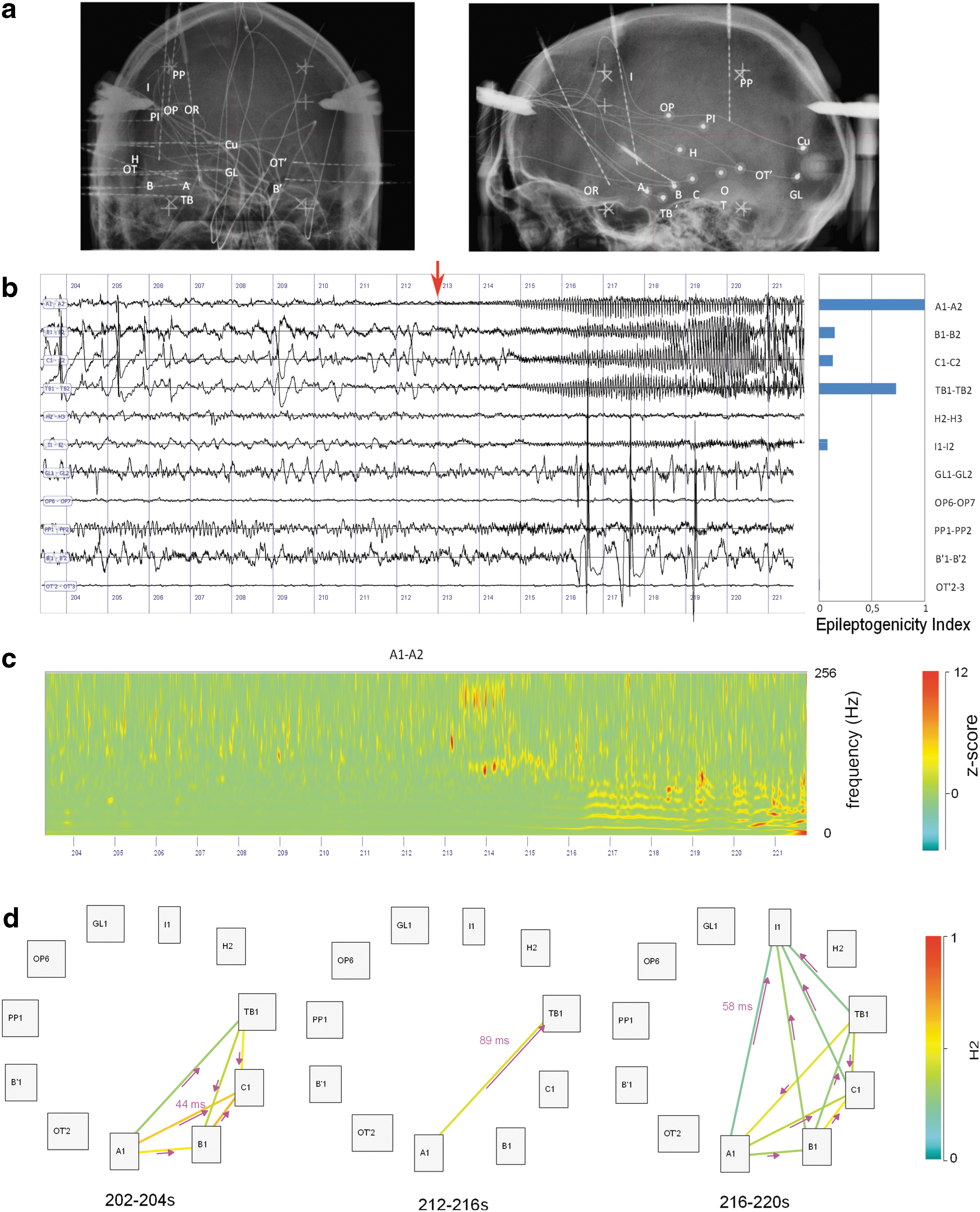
SEEG recordings were performed, thanks to intracerebral electrodes with multiple contacts (10–15 contacts). These electrodes were implanted according to Talairach stereotaxic method (Talairach and Bancaud, 1973). The electrodes were positioned in each patient based upon hypotheses about the localization of the epileptogenic zone, formulated from available noninvasive information. An example of SEEG implantation is presented in Figure 1a along with representative recording of one seizure (Fig. 1b, c). Each patient had a comprehensive evaluation, including detailed history, neurological examination, neuropsychological testing, high-resolution magnetic resonance imaging (MRI), and video EEG recording of seizures before SEEG. Recordings were carried out between 2001 and 2014. Signals were recorded on a 128- or 256-channel Deltamed™ system. They were originally sampled at 256, 612, or 1024 Hz according to the period of recording. The total number of recorded contacts ranged between 90 and 178. In total, 24 seizures were selected for this study (2 seizures by patient). An average of 12 bipolar channels (range 10–15) were selected per patient based on their involvement during preictal and ictal activity. The SEEG electrodes are labeled according to their target cerebral structure. Electrode labels are listed in Table 2. The letter p (for “prime”) indicates the left side.

FIG. 1.

Findings for patient LAL. (a) Implantation of SEEG electrodes (for nomenclature, see Materials and Methods section). (b) Example of seizure (red arrow indicates the seizure start). The most epileptogenic regions, as indicated by the EI, are A1-A2 (amygdala) and TB1-TB2 (temporal base). (c) Time–frequency representation of the seizure; increase of high-frequency activity at seizure onset is visible on channel A1-A2. (d) Examples of h ² graphs corresponding to different time windows during the seizure. The delay between channels permits to estimate a direction for each link. In the graphs, we counted the number of ingoing and outgoing links for each channel. EI, Epileptogenicity Index; SEEG, stereotaxic electroencephalography. Color images available online at www.liebertpub.com/brain

Table 2.

List of Stereotaxic Electroencephalography Electrodes with Corresponding Anatomical Location

A	Amygdala
B	Anterior hippocampus
C	Posterior hippocampus
Cu	Cuneus
CC	Area 24
GC	Cingulate gyrus
GL	Lingual gyrus
GPH	Parahippocampal gyrus
GSM	Supramarginal gyrus
H	Heschl gyrus
L	Lesion
LP	Paracentral lobe
OF	Frontal operculum
OP	Parietal operculum
OR	Orbitofrontal
OT	Occipitotemporal
PM	Premotor cortex
PA	Area 7a, superior parietal lobule
PP	Area 7b superior parietal lobule
PT	Temporal pole
R	Frontopolar region
SC	Central precentral region
SA	Supplementary motor area
T	Superior temporal gyrus
TB	Temporobasal region
TBa	Entorhinal cortex
TP	Temporal pole

SEEG analysis

Definition of period of interest

Signals were reviewed with the AnyWave software (Colombet et al., 2015) (available at http://meg.univ-amu.fr/wiki/AnyWave). The seizure onset was characterized by the low-voltage rapid discharge (LVRD), which is a transient phenomenon that lasts for few seconds. LVRD was delimited by an experienced neurologist (F.B.) through visual inspection. This period is referred to as the DRD (“during rapid discharge”) period. The period of 8 sec immediately preceding the DRD period is the BRD (“before rapid discharge”) period (Bartolomei et al., 2004). All analyses were performed with a bipolar derivation (subtraction of consecutive channels).

Data were classified visually on the original traces as containing “preictal spiking” if there were spikes occurring simultaneously on several channels.

Nonlinear correlation (h² )

Signals were selected with the AnyWave software (Colombet et al., 2015). They were then exported to MATLAB, and resampled to a common rate of 200 Hz. Several filter settings were used, either large band (1–40 Hz) or within specific frequency bands (4–8, 8–12, 15–40 Hz).

A nonlinear regression analysis was computed based on the h ² index (Bartolomei et al., 2001; Lopes da Silva et al., 1989; Wendling et al., 2001b). In summary, a piecewise linear regression is performed between each pair of signals, testing all the shifts of one signal relative to the other within a maximum lag. The h ² is the coefficient of determination, which measures the goodness of fit of the regression—equivalent to the r ² used in linear regression. For two signals x and y, the piecewise linear approximation f of the transfer function between x and y is defined by: \documentclass{aastex}\usepackage{amsbsy}\usepackage{amsfonts}\usepackage{amssymb}\usepackage{bm}\usepackage{mathrsfs}\usepackage{pifont}\usepackage{stmaryrd}\usepackage{textcomp}\usepackage{portland, xspace}\usepackage{amsmath, amsxtra}\pagestyle{empty}\DeclareMathSizes{10}{9}{7}{6}\begin{document} \begin{align*}{y_{n - \tau }} = f \left( {{x_n}} \right) + {e_n}\end{align*} \end{document}

with n sample number, τ delay between x and y, f the piecewise linear approximation of y, and e error term. The number of segments is typically taken as 10. The h ² measures the proportion of the original sum of square that is explained by the approximation f: \documentclass{aastex}\usepackage{amsbsy}\usepackage{amsfonts}\usepackage{amssymb}\usepackage{bm}\usepackage{mathrsfs}\usepackage{pifont}\usepackage{stmaryrd}\usepackage{textcomp}\usepackage{portland, xspace}\usepackage{amsmath, amsxtra}\pagestyle{empty}\DeclareMathSizes{10}{9}{7}{6}\begin{document} \begin{align*} { h^2 } ( \tau ) = 1 - { \frac { \mathop \sum \limits_n { { { \left( { { y_ { n - \tau } } - f ( { x_n } ) } \right) } ^2 } } } { \mathop \sum \limits_n { { y_ { n - \tau } } ^2 } } } \end{align*} \end{document}

The h ² is bounded between 0 (no correlation) and 1 (maximal correlation) and—contrary to the r ²—is not symmetric (Wendling et al., 2001b). We set the maximum delay to τ _max = 100 msec. For each pair, we retained the maximal value between the two directions h ² _1->2 and h ² _2->1. This value corresponded to a delay between signals, which was used to define the direction of the link (example in Fig. 1d).

Node strength of h² graphs

For all the selected channels (each channel is a bipolar SEEG derivation), we computed all the pairwise h ² values (for the selection of channels, see SEEG recordings section). To illustrate the dynamic changes in graph values, we used a sliding window of length 4 sec and a step of 2 sec. For the receiver operating characteristic (ROC) analysis (see below), we used an 8 sec window to obtain a single value for the preictal period. This produced binary graphs (a link is 0 or 1), with each node corresponding to a channel, and a direction given by the delay. Then, in each time window and for each channel (i.e., graph node), we summed the h ² of all the ingoing links (IN strength), all the outgoing links (OUT value), and all links independently of their direction (total strength TOT) (Barrat et al., 2004).

The relevance of a given node, that is, its importance to serve as a “driver” of epileptic discharges, was estimated by different measures: OUT, OUT/IN, and OUT-IN. This stems from the hypothesis that a leading region is expected to have more outgoing links than ingoing links.

Seizure onset: the EI

High-frequency oscillations are frequently observed during the transition from interictal to ictal activity. They are often referred to as “rapid discharge.” A quantitative measure used clinically in our epilepsy unit is the EI. This index permits to quantify the epileptogenicity in recorded structures, based on criteria that are classically used in visual inspection of SEEG traces by clinicians. It is based both on: (1) the relative energy of the rapid discharge (high-frequency content) measured as an energy ratio (ER) between high and low frequencies and (2) the delay of appearance N_di of this discharge with respect to seizure onset N₀ (Bartolomei et al., 2008): \documentclass{aastex}\usepackage{amsbsy}\usepackage{amsfonts}\usepackage{amssymb}\usepackage{bm}\usepackage{mathrsfs}\usepackage{pifont}\usepackage{stmaryrd}\usepackage{textcomp}\usepackage{portland, xspace}\usepackage{amsmath, amsxtra}\pagestyle{empty}\DeclareMathSizes{10}{9}{7}{6}\begin{document} \begin{align*}E { I_i } = \frac { 1 } { { { N_ { di } } - { N_0 } + 1 } } \mathop \sum \limits_ { n = { N_ { di } } } ^ { { N_ { di } } + H } { ER ( n ) } \end{align*} \end{document}

where i stands for the channel number, H the size of the sliding window over which the ER is averaged.

The EI is a normalized quantity (ranging from 0 to 1). The sliding window on which the ER was computed was set to H = 5 sec to detect the onset of rapid discharges (Bartolomei et al., 2008).

ROC analysis

We tested the capacity of each measure to serve as a detector of epileptogenicity using ROC analysis, a classical test for assessing detectors. EI was thresholded at 0.3, a heuristic threshold derived from experience (Bartolomei et al., 2010). Graph strength measures were normalized between 0 and their maximum value (set to 1). Several thresholds were tested on each graph measure, and the true positive rate (TPR) and false positive rate (FPR) were computed. The ROC curve consists in plotting the TPR (sensitivity) as a function of TPR (1-specificity). A good detector reaches rapidly a high sensibility (high TPR) while keeping a good specificity (low FPR). The quality of the detector can thus be quantified by the area under the ROC curve (area under the curve [AUC]) (Grova et al., 2006). Results of the ROC analyses are presented with boxplots (Advanced boxplot toolbox; http://alex.bikfalvi.com/research/advanced_matlab_boxplot/), and differences between conditions were tested with a Wilcoxon rank sum test (ranksum function of Matlab). Both these procedures are robust to outliers and non-gaussianity, contrary to classical bar plots (https://garstats.wordpress.com/2016/03/09/one-simple-step-to-improve-statistical-inferences/).

Results

We computed graph measures for all preictal periods of all patients with the two different filter settings (1–40 or 15–40 Hz). The correspondence between electrode labels and the anatomical location is listed in Table 2.

Figure 2 shows two seizures corresponding to the two conditions in the same patient, with or without preictal spiking (as identified visually). The increased preictal synchrony in the right column is visible on the h ² graphs in the period immediately preceding the fast discharge (t = 36–38 sec). Patterns of EIs are similar in the two seizures, with higher EI values at PT3-PT4, TBa2-TBa3, and B3-B4. In the “no preictal spiking” case (Fig. 2, left column), increased OUT strength is visible in B3-B4 and TBa2-TBa3. In the “preictal spiking” case (right column) preictal synchrony is also visible on the OUT graphs at t = 36–38 sec in channel PT3-PT4. In the IN graphs (Fig. 2c, right column), it is interesting to note that the TBa2-TBa3 channel has high values just before the seizure onset, in both cases (with or without visible preictal synchrony), which corresponds to the channel with maximum EI.

FIG. 2.

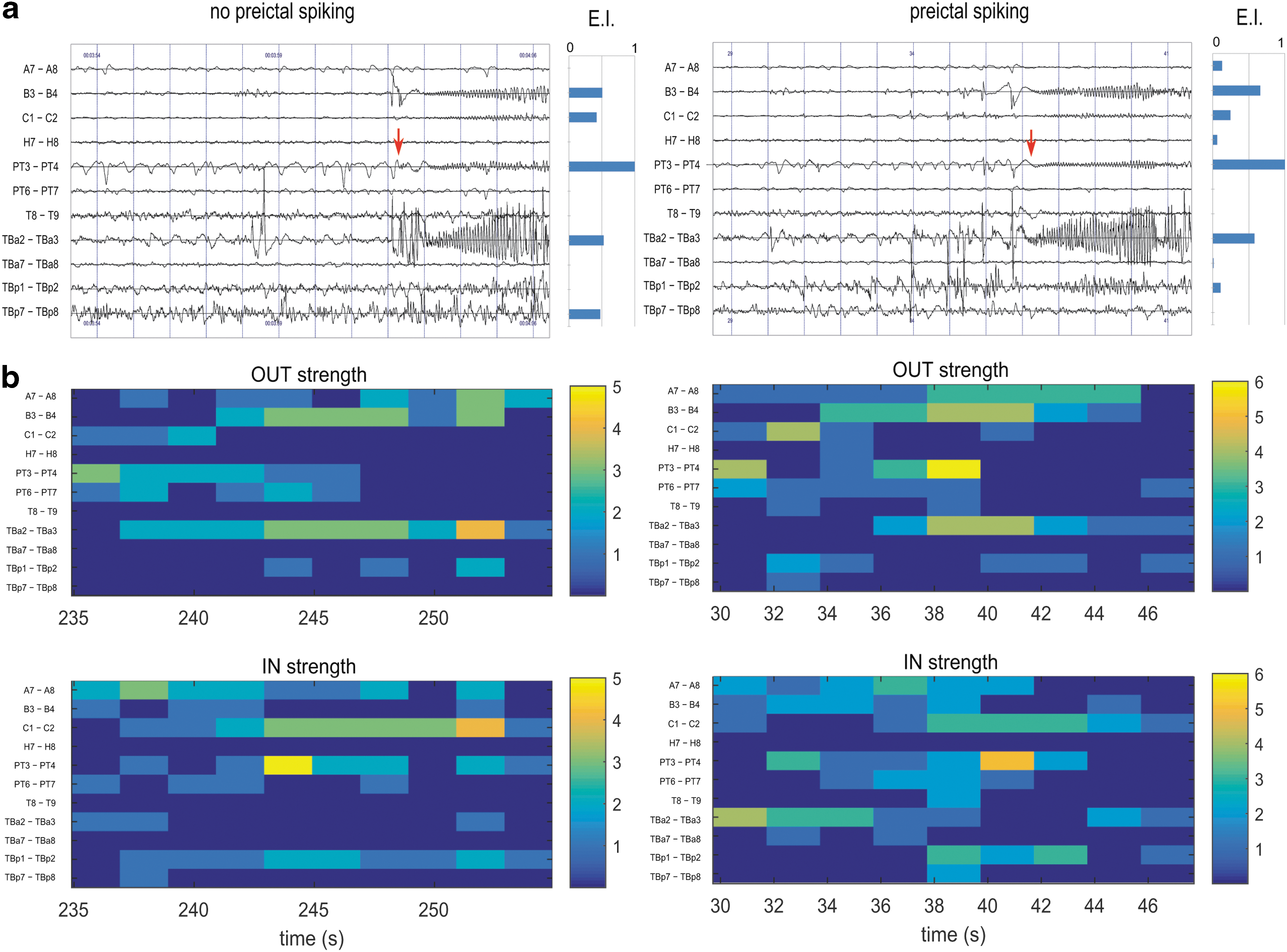
Impact of preictal spiking on synchrony (patient ARR; left column: without preictal spiking, right column with spiking). (a) Seizures on selected channels. Red arrow indicates the seizure start. (b) OUT and IN graph strength. In the “preictal spiking” case, increase in OUT strength can be seen just before the seizure start in the channels corresponding to high EI values (B3-B4, PT3-PT4, TBa2-TBa3). In the “no preictal spiking” case, the OUT strength is low in the channel with higher EI. Interestingly, there are high IN strength values in channels with higher EI value in both cases (PT3-PT4). Color images available online at www.liebertpub.com/brain

As preictal data can present a mixture of low frequencies (slow waves, delta, or theta rhythm) and spikes, we filtered the data in the 15–40 Hz band to be more sensitive to spiking activity. Figure 3 presents a case where this leads to dramatic improvement of the match between graph measures and EI. In Fig. 3a, the preictal and seizure start periods are shown together with the EI values. In the 38–45 s period (preictal phase) on the large-band data, there is a burst of very sharp spikes mixed with low-frequency oscillation at around 1.5 Hz. In the OUT graphs corresponding to the large band activity (Fig. 3b), there is a widespread spatial pattern with high values, with maximal values at SC10-11 and LP7-8, which corresponds to channels with an EI of zero. In contrast, data filtered in the 15–40 Hz band (Fig. 3c) points to regions that correspond well to those with high EI (LP1-LP2 and SC1-SC2).

FIG. 3.

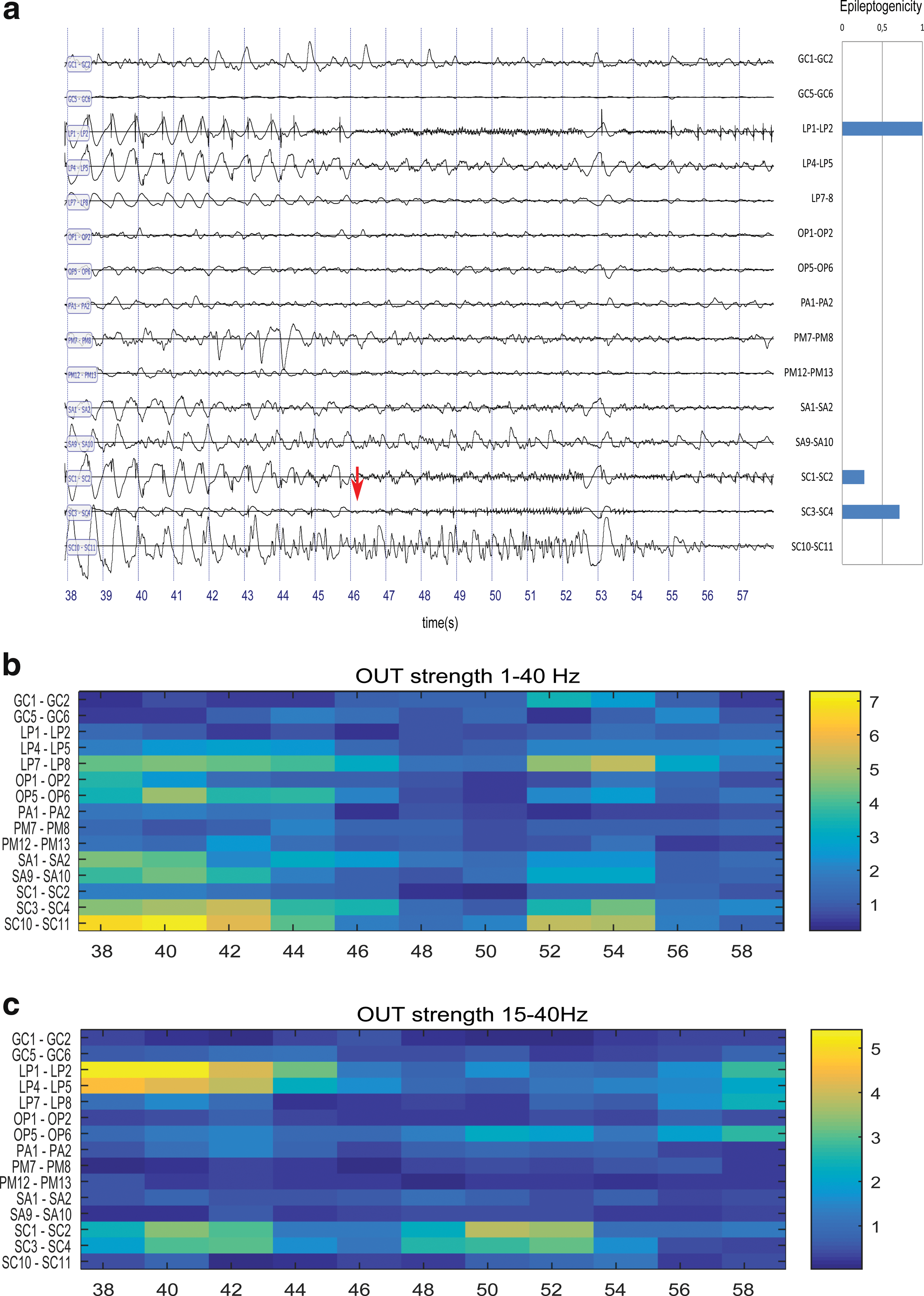
Effect of filtering (patient GAL). (a) The seizure presents clear rythmic spike-and-wave activity in the preictal phase. Red arrow indicates the seizure start. (b) In the OUT degrees filtered in the 1–40 Hz band, there is a widespread spatiotemporal pattern with high values, which does not match the high EI values. The graph measures have likely been sensitive to the prominent slow-frequency activity, which does not seem to have localizing value in this case. (c) In the data filtered in the 15–40 Hz band, high values are obtained in the LP1-LP2 region and SC1-SC2 region, which matches well the EI values. Color images available online at www.liebertpub.com/brain

Figure 4 presents the results of the ROC analysis on the different graph strength measures. In Figure 4a, all seizures are included, whether presenting visible interictal synchrony or not. For all the frequency sub-bands, there is a tendency for the OUT measure to give better results than IN measures (the only significant difference is for the 15–40 Hz, at p < 0.05 with Bonferroni correction for multiple comparisons). The TOT measure is also a good detector, whereas this is not the case for the “leadership” measures (OUT-IN and OUT/IN). The best results are obtained for OUT and TOT measure in the 15–40 Hz sub-band. In Figure 4b, only seizures with visible interictal synchrony are shown. Difference between OUT and IN measure is significant for both 8–12 Hz and 15–40 Hz bands (p < 0.05 for a Wilcoxon rank sum test with Bonferroni correction for multiple comparisons).

FIG. 4.

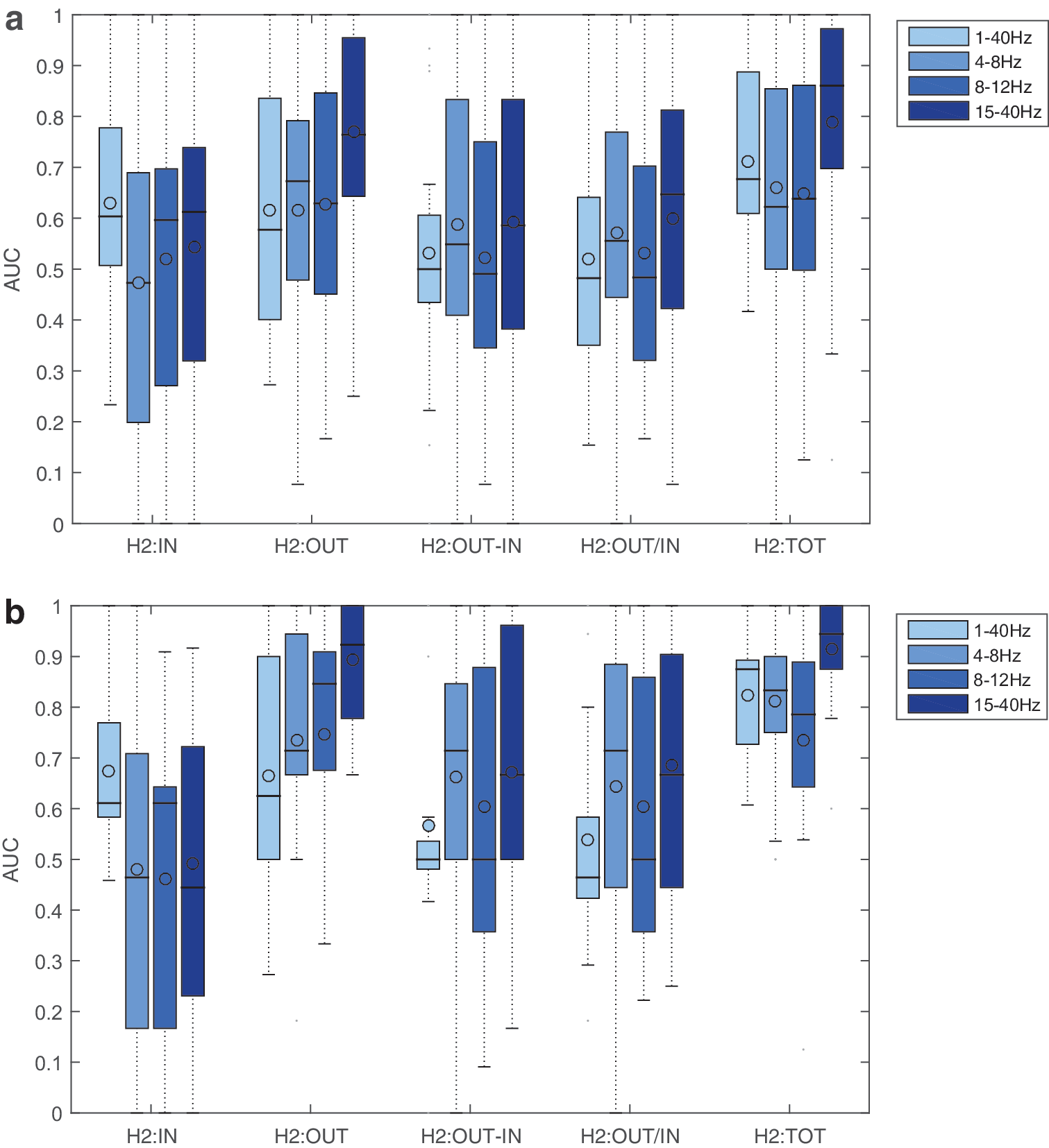
Receiver operating characteristic study of the different strength measures, for several filter settings and preictal spiking conditions. The reference is the list of EI values, with a threshold of 0.3. The AUC was computed under the different settings and conditions. (a) All contacts, independently of whether they present preictal spiking. The best results were obtained for the OUT and TOT measures for the 15–40 Hz filter. (b) Only contacts presenting preictal spiking. All measures based on OUT strength (OUT, OUT-IN, OUT/IN, and TOT) are improved, especially for the 15–40 Hz filter. AUC, area under the curve. Color images available online at www.liebertpub.com/brain

In these results, we used a fixed EI threshold of 0.3, a heuristic value that was obtained from previous experience (Bartolomei et al., 2010). In Supplementary Fig. S1, we show the impact of the EI threshold on the AUC for the OUT and TOT measures. The best concordance was obtained for EI thresholds ranging from 0.1 to 0.4.

In Figure 5, we map the relationships between EI and the best graph measures (OUT and TOT). To be noted, all graph measures have been normalized with respect to the higher value in a given seizure (giving values in the 0–1 range). This permits to investigate qualitatively what thresholds could be used, and what are the sensitivity and specificity or the measures in different conditions (with or without preictal spiking). For all condition and measures, there is a large proportion in the “high values” quadrant (graph measures greater than 0.5 and EI >0.5). This corresponds to the contacts with a good match between the measures (OUT or TOT) and the EI, and to the true positive detections in the ROC study. For the OUT, TOT, and “TOT with preictal spiking” measure, there is, however, a large number of contacts with high measure values (>0.5) and low EI (<0.5). This corresponds to false detections in the ROC study. The OUT measure with preictal spiking has better specificity (few contacts in the “false detection” quadrant), but at the expense of more missed detections (OUT <0.5 and EI >0.5 quadrant).

FIG. 5.

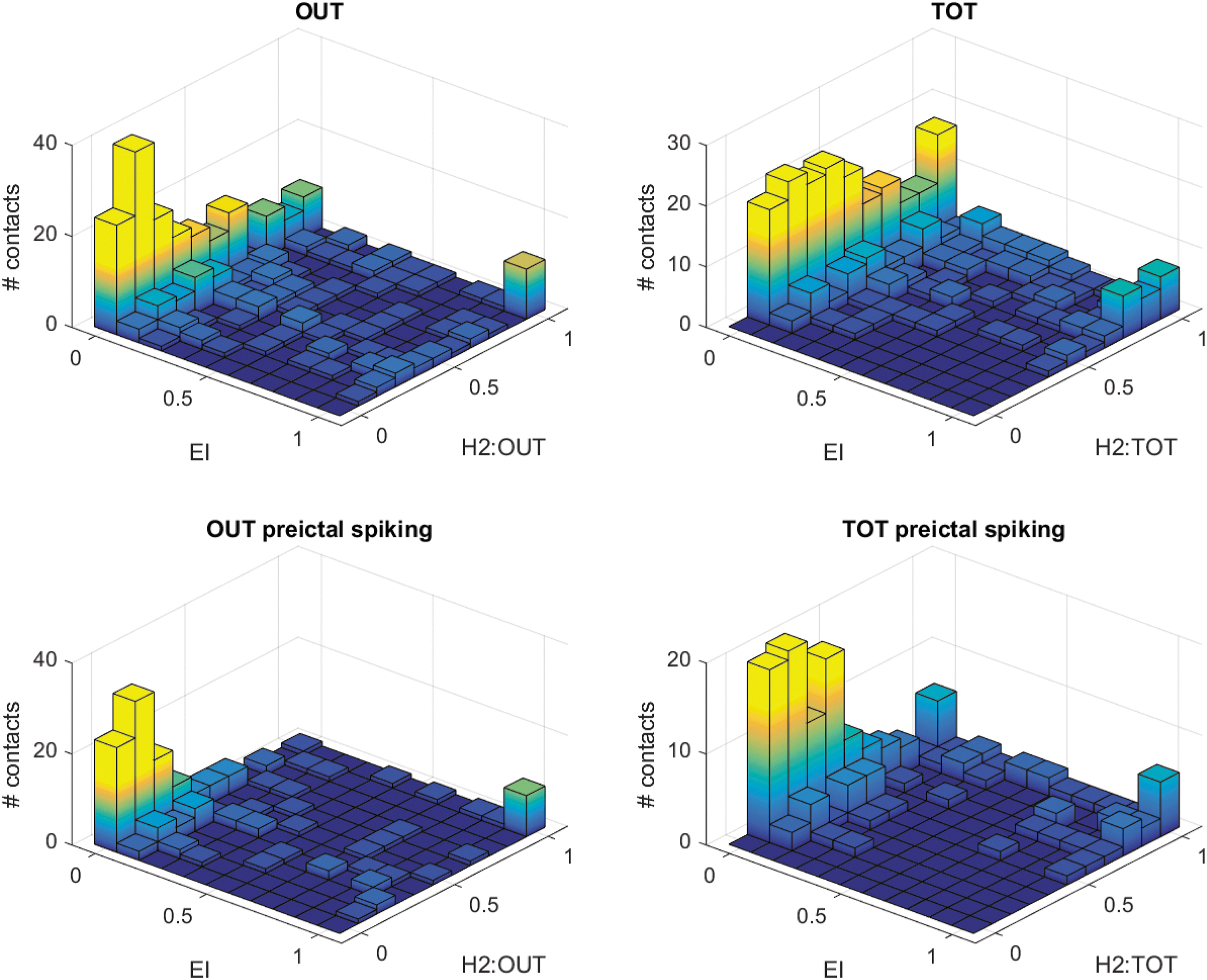
Joint histogram of OUT or TOT graph strength measures and EI. For each patient, measures were normalized by the maximal value across electrodes (relative strength). Top line: all contacts are included. A large proportion of values lie either in the low value quadrant (EI and relative strength <0.5) or high value quadrant (EI and relative strength >0.5). Bottom line: only contacts with preictal spiking were included. In this configuration, values have less dispersion. The OUT measure has better specificity (less values in the EI <0.5 and strength >0.5 quadrant), but less sensitivity (more values in the EI >0.5 and OUT <0.6 quadrant). Color images available online at www.liebertpub.com/brain

Discussion

We found in the present study that patterns of hypersynchrony are visible in SEEG during the preictal period in a large proportion of seizures. This confirms the study by Bartolomei and colleagues performed in the particular case of medial temporal lobe epilepsy (Bartolomei et al., 2004). Here, we extend this work to other types of epilepsies, with larger number of nodes taken into account in the analysis of networks. Moreover, we use various graph measures of IN and OUT strength (van Mierlo et al., 2013; Wilke et al., 2011), which allowed quantifying the leading nodes in the network.

Concordance between measures and EI

We observed that, in a large proportion of cases, the out strength (OUT) and total strength (TOT) measures in the preictal period match the seizure onset zone as defined by the EI. This is consistent with the findings of Van Mierlo and colleagues (2013), which were obtained on mixed electrocorticography/intracerebral recordings with a different connectivity method and a visual analysis of the epileptogenic zone. Our findings extend to an SEEG setting, which are recordings directly within the brain structures, using EI as a quantified way to assess the extent of the rapid discharge at seizure onset.

The fact that TOT gives the best results (especially in the case with precital spiking), compared with OUT and IN taken separately, suggests that there is an interaction between measures: the best marker is when there are both a high number of OUT and a high number of IN. This is plausible, because a region that receives many incoming links without driving other regions may not be hyperexcitable. Future modeling work could help understanding better such phenomenon (Proix et al., 2014).

The best concordance between OUT and EI was seen for the high-pass filtered data in the 15–40 Hz band. This suggests that the best marker of epileptogenicity may reside in the fast part of epileptic spike activity—the spike per se—and not the following slow wave, which may involve large networks and be less specific spatially. In line with this, Sato and colleagues have found a decrease of the slow frequency content of spikes with respect to high frequencies in the preictal period (Sato et al., 2014). Concordance was also higher for seizures with visible preictal synchronous discharges. These discharges correspond to highly synchronous pathological activity, which potentially constitute the best marker for hyperexcitable tissues. Changes in synchrony associated with preictal spiking have already been shown (Bartolomei et al., 2004). Still, it is important to note that previous studies have found abnormal synchrony that could be a surrogate of epileptogenic tissues independently of the presence of interictal spiking (Bettus et al., 2008). This indicates that the graph analysis of networks outside of spikes could potentially be a source of information on the level of excitability of brain regions.

Delineation of epileptogenic tissues

We used the EI as a reference measure to which graph measures were compared. From a fundamental perspective, such good concordance suggests that there could be common mechanisms between the synchrony building up immediately before the seizure and the actual fast discharge—the hallmark of seizure onset. From a clinical point of view, graph measures could be a new way to delineate the extent of the epileptogenic zone based on preictal activity. The EI requires a somehow arbitrary threshold, and is dependent on several parameters (for the detection of increase of energy, or for the weighting between energy increase and time). Graph measures also rely on thresholding, but arise from a completely different—and thereby complementary—source of information. In addition, the EI is a measure that cannot be applied in seizures starting by clonic or slower discharges, which represent in our center around 20% of the seizure onset patterns recorded with SEEG. In these cases, connectivity measures could be more suited for the quantification of the seizure onset zone.

An important question that is raised in the context of epileptic patients is the influence of antiepileptic drugs on IN/OUT strength. Douw and colleagues have reported no dependence of functional connectivity at rest on the dose of antiepileptic drug (Douw et al., 2010). Moreover, during SEEG, antiepileptic drugs are typically reduced, which should further lower the potential impact.

Limitations and future directions

In this study, we avoided as much as possible the used thresholds, which are difficult to tune as pointed above. Thus, we used node strength (sum of values) instead of node degrees (number of significant links), and we performed an ROC analysis that is independent of the choice of a threshold. However, as the goal of signal processing methods is to quantify the actual extent of epileptogenic tissues, this sets the emphasis on selecting a proper threshold. Further work will be required to find a correct null hypothesis to threshold the graph measures, which is a difficult issue (van Wijk et al., 2010).

It will be important to extend our results to the interictal period. Interictal activity is known to often involve large brain areas, which can be different from the epileptogenic zone (Bartolomei et al., 2016). Graph measures could, therefore, be a way to emphasize the important nodes within the interictal network (Malinowska et al., 2014). Proving that interictal graph measures are also a good marker of seizure onset would lower the need to record seizures—which would be of great importance for presurgical evaluation, either invasive or noninvasive.

Other measures of connectivity have been proposed in the literature. In particular, there is a growing interest in Granger Causality measures (Bressler and Seth, 2011) that assess whether incorporating the past from a signal from another channel improves the prediction of the signal in a channel of interest. Thus, several variants of connectivity have been applied to epilepsy (Amini et al., 2011; Coito et al., 2015; Epstein et al., 2014). It is interesting to note that Granger causality as implemented with autoregressive models (Brovelli et al., 2004) or with a covariance-based approach (Brovelli et al., 2015) may not be radically different from a classical correlation analysis (Davey et al., 2013). What is likely to be a more influential choice is the fact of considering pairwise or multivariate methods, which could remove indirect correlation arising from a common driving node (Kuś et al., 2004). Another promising venue is to investigate high-frequency oscillations (Epstein et al., 2014). Such high frequencies have been shown to be a good marker of the epileptogenic zone (Urrestarazu et al., 2007), but require careful handling of the frequency overlap between epileptic spikes and oscillations (Bénar et al., 2010; Jmail et al., 2011). Further work is needed to test the impact of these methodological choices.

Summary

In summary, our results suggest that the OUT and TOT graph measures on h ² in the preictal period can be used as additional quantities for assessing the epileptogenicity of the different brain areas. As the threshold on EI is difficult to set, graph measures performed on preictal spikes constitute additional information that could potentially help delineating the regions to be resected, better than plain counting of preictal spikes. Such mapping would then correspond to a “primary irritative zone” (Badier and Chauvel., 1995; Malinowska et al., 2014). Future directions will be to extend this study to the different interictal patterns, taking into account the variability in dynamics observed across time and brain states.

Footnotes

Acknowledgment

Part of this work was funded by a joint Agence Nationale de la Recherche (ANR) and Direction Génerale de l'Offre de Santé (DGOS) under grant “VIBRATIONS” ANR 13 PRTS 0011 01.

Author Disclosure Statement

No competing financial interests exist.

References

Amini

, Jutten

, Achard

, David

, Soltanian-Zadeh

, Hossein-Zadeh

, et al. 2011. Directed differential connectivity graph of interictal epileptiform discharges. IEEE Transact Biomed Eng, 58:884–893.

Andrzejak

, David

, Gnatkovsky

, Wendling

, Bartolomei

, Francione

, et al. 2014. Localization of epileptogenic zone on pre-surgical intracranial EEG recordings: toward a validation of quantitative signal analysis approaches. Brain Topogr, 28:832–837.

Badier

, Chauvel

. 1995. Spatio-temporal characteristics of paroxysmal interictal events in human temporal lobe epilepsy. J Physiol, 89:255–264.

Barrat

, Barthelemy

, Pastor-Satorras

, Vespignani

. 2004. The architecture of complex weighted networks. Proc Natl Acad Sci U S A, 101:3747–3752.

Bartolomei

, Chauvel

, Wendling

. 2008. Epileptogenicity of brain structures in human temporal lobe epilepsy: a quantified study from intracerebral EEG. Brain, 131:1818–1830.

Bartolomei

, Cosandier-Rimele

, McGonigal

, Aubert

, Regis

, Gavaret

, et al. 2010. From mesial temporal lobe to temporoperisylvian seizures: a quantified study of temporal lobe seizure networks. Epilepsia, 51:2147–2158.

Bartolomei

, Guye

, Wendling

. 2013. Abnormal binding and disruption in large scale networks involved in human partial seizures. EPJ Nonlinear Biomed Phys, 1:1–16.

Bartolomei

, Trebuchon

, Bonini

, Lambert

, Gavaret

, Woodman

, et al. 2016. What is the concordance between the seizure onset zone and the irritative zone? A SEEG quantified study. Clin Neurophysiol, 127:1157–1162.

Bartolomei

, Wendling

, Bellanger

, Régis

, Chauvel

. 2001. Neural networks involving the medial temporal structures in temporal lobe epilepsy. Clin Neurophysiol, 112:1746–1760.

10.

Bartolomei

, Wendling

, Regis

, Gavaret

, Guye

, Chauvel

. 2004. Pre-ictal synchronicity in limbic networks of mesial temporal lobe epilepsy. Epilepsy Res, 61:89–104.

11.

Bénar

, Chauvière

, Bartolomei

, Wendling

. 2010. Pitfalls of high-pass filtering for detecting epileptic oscillations: a technical note on “false” ripples. Clin Neurophysiol, 121:301–310.

12.

Bettus

, Wendling

, Guye

, Valton

, Régis

, Chauvel

, et al. 2008. Enhanced EEG functional connectivity in mesial temporal lobe epilepsy. Epilepsy Res, 81:58–68.

13.

Bressler

, Seth

. 2011. Wiener-Granger causality: A well established methodology. Neuroimage, 58:323–329.

14.

Brovelli

, Chicharro

, Badier

, Wang

, Jirsa

. 2015. Characterization of cortical networks and corticocortical functional connectivity mediating arbitrary visuomotor mapping. J Neurosci, 35:12643–12658.

15.

Brovelli

, Ding

, Ledberg

, Chen

, Nakamura

, Bressler

. 2004. Beta oscillations in a large-scale sensorimotor cortical network: directional influences revealed by Granger causality. Proc Natl Acad Sci U S A, 101:9849–9854.

16.

Coito

, Plomp

, Genetti

, Abela

, Wiest

, Seeck

, et al. 2015. Dynamic directed interictal connectivity in left and right temporal lobe epilepsy. Epilepsia, 56:207–217.

17.

Colombet

, Woodman

, Badier

, Benar

. 2015. AnyWave: a cross-platform and modular software for visualizing and processing electrophysiological signals. J Neurosci Methods, 242:118–126.

18.

Davey

, Grayden

, Gavrilescu

, Egan

, Johnston

. 2013. The equivalence of linear Gaussian connectivity techniques. Hum Brain Mapp, 34:1999–2014.

19.

Douw

, van Dellen

, de Groot

, Heimans

, Klein

, Stam

, et al. 2010. Epilepsy is related to theta band brain connectivity and network topology in brain tumor patients. BMC Neurosci, 11:103.

20.

Epstein

, Adhikari

, Gross

, Willie

, Dhamala

. 2014. Application of high-frequency Granger causality to analysis of epileptic seizures and surgical decision making. Epilepsia, 55:2038–2047.

21.

Grova

, Daunizeau

, Lina

, Bénar

, Benali

, Gotman

. 2006. Evaluation of EEG localization methods using realistic simulations of interictal spikes. Neuroimage, 29:734–753.

22.

Jmail

, Gavaret

, Wendling

, Kachouri

, Hamadi

, Badier

J-M

, et al. 2011. A comparison of methods for separation of transient and oscillatory signals in EEG. J Neurosci Methods, 199:273–289.

23.

Kuś

, Kamiński

, Blinowska

. 2004. Determination of EEG activity propagation: pair-wise versus multichannel estimate. IEEE Trans Biomed Eng, 51:1501–1510.

24.

Lopes da Silva

, Pijn

, Boeijinga

. 1989. Interdependence of EEG signals: linear vs. nonlinear associations and the significance of time delays and phase shifts. Brain Topogr, 2:9–18.

25.

Malinowska

, Badier

, Gavaret

, Bartolomei

, Chauvel

, Benar

. 2014. Interictal networks in magnetoencephalography. Hum Brain Mapp, 35:2789–2805.

26.

Ponten

, Bartolomei

, Stam

. 2007. Small-world networks and epilepsy: graph theoretical analysis of intracerebrally recorded mesial temporal lobe seizures. Clin Neurophysiol, 118:918–927.

27.

Proix

, Bartolomei

, Chauvel

, Bernard

, Jirsa

. 2014. Permittivity coupling across brain regions determines seizure recruitment in partial epilepsy. J Neurosci, 34:15009–15021.

28.

Sato

, Doesburg

, Wong

, Boelman

, Ochi

, Otsubo

. 2014. Preictal surrender of post-spike slow waves to spike-related high-frequency oscillations (80–200 Hz) is associated with seizure initiation. Epilepsia, 55:1399–1405.

29.

Schwartz

, Hong

S-B

, Bagshaw

, Chauvel

, Bénar

C-G

. 2011. Preictal changes in cerebral haemodynamics: review of findings and insights from intracerebral EEG. Epilepsy Res, 97:525–266.

30.

Stefan

, Lopes da Silva

. 2013. Epileptic neuronal networks: methods of identification and clinical relevance. Front Neurol, 4:8.

31.

Talairach

, Bancaud

. 1973. Stereotaxic approach to epilepsy: methodology of anatomo-functional stereotaxic investigations. Progr Neurol Surg, 5:297–354.

32.

Urrestarazu

, Chander

, Dubeau

, Gotman

. 2007. Interictal high-frequency oscillations (100–500 Hz) in the intracerebral EEG of epileptic patients. Brain, 130:2354–2366.

33.

van Mierlo

, Carrette

, Hallez

, Raedt

, Meurs

, Vandenberghe

, et al. 2013. Ictal-onset localization through connectivity analysis of intracranial EEG signals in patients with refractory epilepsy. Epilepsia, 54:1409–1418.

34.

van Wijk

, Stam

, Daffertshofer

. 2010. Comparing brain networks of different size and connectivity density using graph theory. PLoS One, 5:e13701.

35.

Wendling

, Bartolomei

. 2001a. Modeling EEG signals and interpreting measures of relationship during temporal-lobe seizures: an approach to the study of epileptogenic networks. Epileptic Disord Special, Issue:67–78.

36.

Wendling

, Bartolomei

, Bellanger

, Bourien

, Chauvel

. 2003. Epileptic fast intracerebral EEG activity: evidence for spatial decorrelation at seizure onset. Brain, 126:1449–1459.

37.

Wendling

, Bartolomei

, Bellanger

, Chauvel

. 2001b. Interpretation of interdependencies in epileptic signals using a macroscopic physiological model of the EEG. Clin Neurophysiol, 112:1201–1218.

38.

Wilke

, Worrell

, He

. 2011. Graph analysis of epileptogenic networks in human partial epilepsy. Epilepsia, 52:84–93.

Supplementary Material

Please find the following supplemental material available below.

For Open Access articles published under a Creative Commons License, all supplemental material carries the same license as the article it is associated with.

For non-Open Access articles published, all supplemental material carries a non-exclusive license, and permission requests for re-use of supplemental material or any part of supplemental material shall be sent directly to the copyright owner as specified in the copyright notice associated with the article.

0.00 MB

0.04 MB

Graph Measures of Node Strength for Characterizing Preictal Synchrony in Partial Epilepsy

Abstract

Introduction

Materials and Methods

Selection of patients

SEEG recordings

SEEG analysis

Definition of period of interest

Nonlinear correlation (h2 )

Node strength of h2 graphs

Seizure onset: the EI

ROC analysis

Results

Discussion

Concordance between measures and EI

Delineation of epileptogenic tissues

Limitations and future directions

Summary

Footnotes

Acknowledgment

Author Disclosure Statement

References

Supplementary Material

Nonlinear correlation (h² )

Node strength of h² graphs