Spatiotemporal Modeling of Brain Dynamics Using Resting-State Functional Magnetic Resonance Imaging with Gaussian Hidden Markov Model

Abstract

Analyzing functional magnetic resonance imaging (fMRI) time courses with dynamic approaches has generated a great deal of interest because of the additional temporal features that can be extracted. In this work, to systemically model spatiotemporal patterns of the brain, a Gaussian hidden Markov model (GHMM) was adopted to model the brain state switching process. We assumed that the brain switches among a number of different brain states as a Markov process and used multivariate Gaussian distributions to represent the spontaneous activity patterns of brain states. This model was applied to resting-state fMRI data from 100 subjects in the Human Connectome Project and detected nine highly reproducible brain states and their temporal and transition characteristics. Our results indicate that the GHMM can unveil brain dynamics that may provide additional insights regarding the brain at resting state.

Introduction

Understanding the human brain as a dynamical system is gaining traction in the literature (Fox et al., 2005; Rabinovich and Muezzinoglu, 2010), where the human brain is assumed to frequently switch among different metastable states instead of lingering in a single state. Moreover, dynamic approaches, such as sliding window correlation, have shown advantages over stationary ones in detecting neurological diseases, such as schizophrenia (Sakoğlu et al., 2010). These advantages arise from additional features gained by analyzing the brain signals dynamically. Therefore, modeling brain state switching as a dynamic system can unveil additional characteristics about the underlying processes of human brains.

Existing dynamic analysis approaches have limitations. For example, some techniques, such as coactivation patterns (CAPs) (Liu et al., 2013; Liu and Duyn, 2013;), spatial independent component analysis (ICA) (Beckmann et al., 2005), and temporal ICA (Smith et al., 2012) cannot fully exploit information contained in the temporal order of functional magnetic resonance imaging (fMRI) time frames. When the temporal order of fMRI time frames is ignored, each time frame is treated as an independent sample of the brain, and thus shuffling fMRI time frames does not affect the spatial patterns derived by these approaches. In addition, ICA-based approaches assume independence of components and rely on this assumption to derive spatial patterns. Other dynamic methods take the sequential order of fMRI time frames into consideration. For example, the sliding window approach, which has been applied to estimate fluctuations in functional connectivity (Allen et al., 2014), retains sequential information in the data. However, because the length of the sliding window is fixed (Keilholz, 2014), signals from multiple states may be mixed in each window, resulting in contamination between states and maybe even cancellation of signals. While these methods present simple statistics, such as the occurrence rate of CAPs or functional connectivity states, quantification of the sequential transitions between CAPs or states is not embedded in these models.

In contrast, we focus on quantifying the sequential transitions between different brain states using transition probabilities, and model the brain with a Gaussian hidden Markov model (GHMM) (Bilmes, 1998; Eddy, 1996). Assuming the brain transits among different states over time, our GHMM models the state switching process as a Markov chain, and the spontaneous activity pattern of each brain state as a multivariate Gaussian distribution. Unlike ICA, which assumes the components to be independent with each other, our model makes no hypothesis on the relationship between brain states.

The HMM has been previously employed as a sequential modeling tool in studying the brain (Baker et al., 2014; Eavani et al., 2013; Jones et al., 2007; Ou et al., 2014). The HMM was applied to electrophysiological data and detected 4 brain states of neuronal firing patterns in rodents subjected to different types of stimuli (Jones et al., 2007). Applied to human data, the HMM revealed temporal variability of functional connectivity in magnetoencephalography (Baker et al., 2014) and fMRI (Eavani et al., 2013; Ou et al., 2014). A generalized HMM, the hidden Markov random field, was applied in fMRI to detect binary state (on/off) switching on a voxel level (Lindquist et al., 2007; Liu et al., 2014; Robinson et al., 2010).

Compared to the previous applications of HMM in fMRI, our approach is substantially different. The model in Ou and coworkers (2014) was based on the functional connectivity strength derived by the sliding window method, while our model is directly based on fMRI time courses, which will not encounter the aforementioned blurring by the use of sliding window. Although Eavani and coworkers (2013) also modeled fMRI time courses using a HMM, they studied functional connectivity changes using covariance matrices from each state. In contrast, we investigate temporal dynamics of spontaneous brain activity by analyzing the average activity pattern of each state. The hidden Markov random field in (Lindquist et al., 2007; Liu et al., 2014; Robinson et al., 2010) assumed that each voxel had only two states (on/off), whereas our GHMM does not have assumption on the number of states. Furthermore, the criteria for determining the number of states in the previous work was relatively ambiguous with the number of states determined by the elbow point (Eavani et al., 2013) or local optimum (Ou et al., 2014) of the model's log-likelihood. In this study, we introduce a more quantitative and robust method of using stability as a criterion for determining the number of states.

To the best of our knowledge, GHMM has not hitherto been applied to model the sequential state switching process of spontaneous brain activities. The GHMM quantifies the sequential transition of brain states and is not restricted by the aforementioned limitations of CAPs, ICA, and sliding window. In this article, we describe this approach and its application in a comprehensive analysis of brain spontaneous activities based on the publicly available Human Connectome Project (HCP) dataset.

Materials and Methods

Dataset and preprocessing

One hundred subjects from HCP (Van Essen et al., 2013) S500 release were used in the present work (age: 22–36+, gender: 46 male/54 female, TR = 0.72 sec, scan duration: 14.4 min, one scan for each subject). Preprocessing was performed according to the minimal preprocessing pipelines of HCP (Glasser et al., 2013). In particular, we considered the data that had been processed with ICA-FIX (Griffanti, Salimi-Khorshidi et al., 2014; Salimi-Khorshidi et al., 2014), registered onto 32k Cento69 surface mesh (Van Essen et al., 2012), and slightly smoothed with 2 mm half width at half maximum kernel. All time courses were further filtered with a 0.01–0.1 Hz band-pass filter.

To reduce computational complexity, signals from 236 regions of interest (ROIs) (Power et al., 2011) were extracted by averaging time courses of voxels within a 5 mm radius. This distance was calculated based on surface distance by Dijkstra's algorithm (Hanke et al., 2009). The mean value of each time course was subtracted and the standard deviations were normalized to 1 before these time courses were fed into the GHMM.

Brain state switching model

To model resting-state fMRI time courses in a nonstationary manner, we applied a sequential modeling tool, GHMM, to analyze the data. It has been shown that the brain is constantly switching from one metastable state to another (Rabinovich and Muezzinoglu, 2010). In this work, the sequential switching process of brain states was modeled as a Markov chain, while an observation of a brain state (i.e., an fMRI time acquisition) was modeled by a multivariate Gaussian distribution. A toy example illustrating the use of a GHMM with two states is shown in Figure 1. In this example, the brain is switching between two different brain states (introspection state and external processing state), and the observation from fMRI are activations in default mode network (DMN) and dorsal attention network, respectively.

FIG. 1.

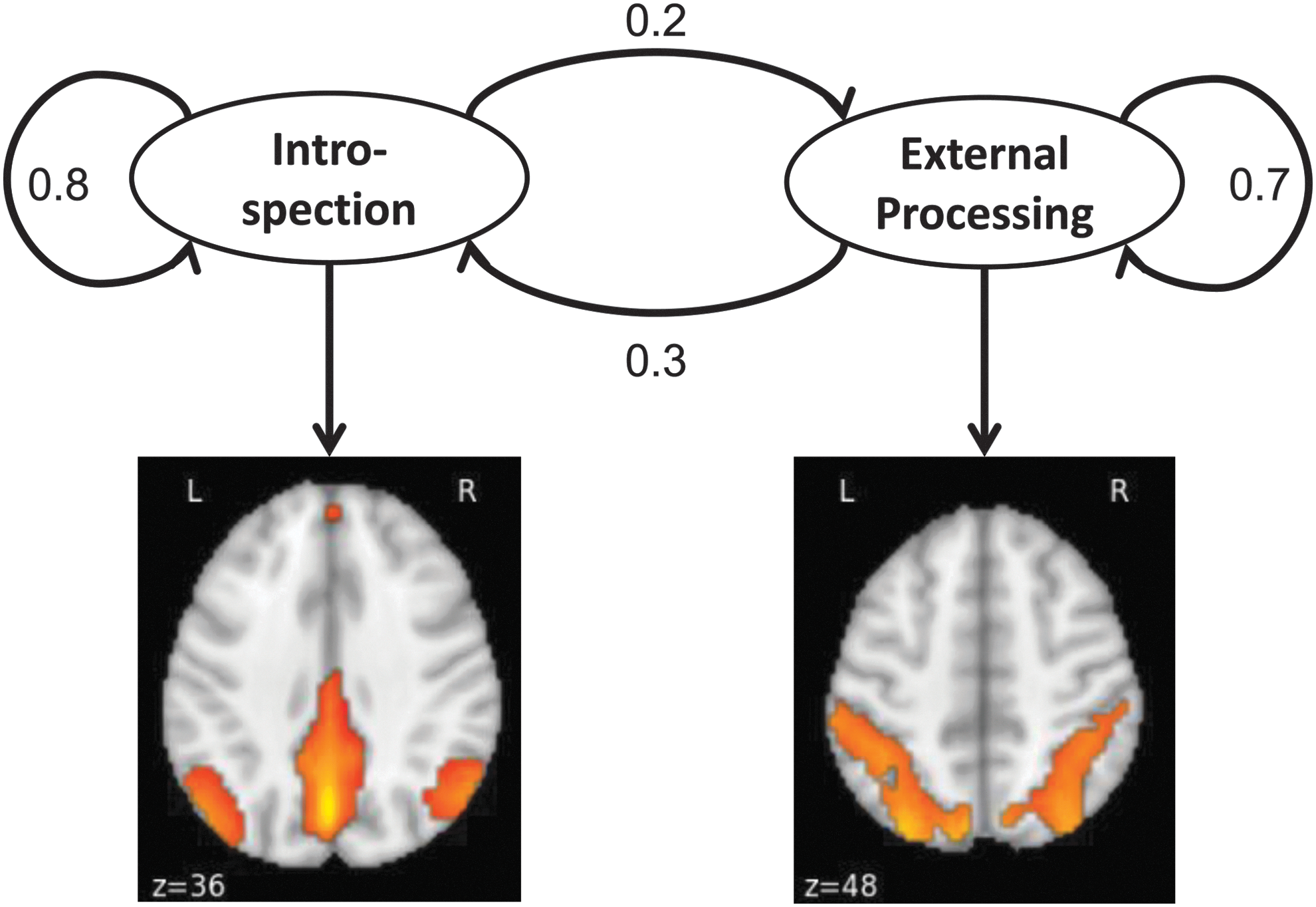
A two-state toy example of the brain's Gaussian hidden Markov model (GHMM). In this case, the brain is only switching between two states, introspection and external processing. The numbers on the arrows represent the probabilities of state switching. During the introspection state, the default mode network is activated, whereas in the external processing state, activation is assumed to be in the dorsal attention network. Color images available online at www.liebertpub.com/brain

To derive the GHMM that best fits the fMRI observations, its parameter set \documentclass{aastex}\usepackage{amsbsy}\usepackage{amsfonts}\usepackage{amssymb}\usepackage{bm}\usepackage{mathrsfs}\usepackage{pifont}\usepackage{stmaryrd}\usepackage{textcomp}\usepackage{portland, xspace}\usepackage{amsmath, amsxtra}\pagestyle{empty}\DeclareMathSizes{10}{9}{7}{6}\begin{document}$$\tilde { \lambda}$$ \end{document} was estimated using the following objective function: \documentclass{aastex}\usepackage{amsbsy}\usepackage{amsfonts}\usepackage{amssymb}\usepackage{bm}\usepackage{mathrsfs}\usepackage{pifont}\usepackage{stmaryrd}\usepackage{textcomp}\usepackage{portland, xspace}\usepackage{amsmath, amsxtra}\pagestyle{empty}\DeclareMathSizes{10}{9}{7}{6}\begin{document} \begin{align*}\tilde { \lambda} = \arg \ { \max}_{ \lambda}\ { \Pi}_{ all\ subjects} \ P ( \textbf{\textit{O}} \mid \lambda ) , \tag{1}\end{align*} \end{document}

where λ is the parameter set for the GHMM; \documentclass{aastex}\usepackage{amsbsy}\usepackage{amsfonts}\usepackage{amssymb}\usepackage{bm}\usepackage{mathrsfs}\usepackage{pifont}\usepackage{stmaryrd}\usepackage{textcomp}\usepackage{portland, xspace}\usepackage{amsmath, amsxtra}\pagestyle{empty}\DeclareMathSizes{10}{9}{7}{6}\begin{document}$$\textbf{\textit{O}} = \{ \textbf{\textit{O}}_t \} , \,t=1 , 2 , \ldots , T$$ \end{document} , are the observations from fMRI and T denotes the total number of fMRI acquisitions per person. P( O |λ) is the probability of obtaining the fMRI observations O given that the parameter set is λ. In the GHMM, the probability of the observations under a state is modeled as a multivariate Gaussian distribution. In our case, the mean vector of the Gaussian distribution represents the average activation pattern of each brain state, and its covariance matrix is used to model the variability within each brain state. With a Gaussian assumption, the objective function can be written as:

the parameters in the above equation are as follows. \documentclass{aastex}\usepackage{amsbsy}\usepackage{amsfonts}\usepackage{amssymb}\usepackage{bm}\usepackage{mathrsfs}\usepackage{pifont}\usepackage{stmaryrd}\usepackage{textcomp}\usepackage{portland, xspace}\usepackage{amsmath, amsxtra}\pagestyle{empty}\DeclareMathSizes{10}{9}{7}{6}\begin{document}$$a_{ij} = P ( q_{t - 1} = i \mid q_t = j )$$ \end{document} denotes the probability of switching from state i to state j. μ _i and Σ _i are the mean vector and covariance matrix of the multivariate Gaussian distribution under state i. \documentclass{aastex}\usepackage{amsbsy}\usepackage{amsfonts}\usepackage{amssymb}\usepackage{bm}\usepackage{mathrsfs}\usepackage{pifont}\usepackage{stmaryrd}\usepackage{textcomp}\usepackage{portland, xspace}\usepackage{amsmath, amsxtra}\pagestyle{empty}\DeclareMathSizes{10}{9}{7}{6}\begin{document}$$\lambda = \{ a_{ij} , {\boldsymbol{\mu}}_i , {\boldsymbol{\Sigma}}_i \} , \,i , j = 1 , 2 , \cdots , M$$ \end{document} , where M is the total number of hidden brain states. N (N = 236) denotes the total number of time courses that are fed into the model and P(q₀ ) represents the initial state probability. \documentclass{aastex}\usepackage{amsbsy}\usepackage{amsfonts}\usepackage{amssymb}\usepackage{bm}\usepackage{mathrsfs}\usepackage{pifont}\usepackage{stmaryrd}\usepackage{textcomp}\usepackage{portland, xspace}\usepackage{amsmath, amsxtra}\pagestyle{empty}\DeclareMathSizes{10}{9}{7}{6}\begin{document}$$\Sigma_{q_0}\, P ( q_0 ) a_{q_0q_1}$$ \end{document} is assumed to be a uniform distribution such that q ₁ can start with any states with equal probability. To further reduce computational complexity, we set the covariance matrix of the multivariate Gaussian to be diagonal, that is, each dimension of the Gaussian distribution is uncorrelated, assuming that the signal changes (noise and individual variability) in different ROIs at each state are uncorrelated.

The observations from fMRI time courses, O , were fed into a k-means clustering program to identify M cluster centers, and the resultant cluster centers were used to initialize the mean of the Gaussian distribution, μ _i. The covariance matrices of the Gaussian, Σ _i, were initialized as the covariance matrix of the first subject's original fMRI time courses. The transition probabilities, a_ij , were set to be equal for all the possible switches. The Baum–Welch algorithm (Rabiner, 1989) was employed to solve the problem in equation (1). Details of the algorithm can be found in Scikit Learning (Pedregosa et al., 2011).

Stability and reproducibility

Different initializations of the Baum–Welch algorithm may lead to convergence into different local optima. To address this issue, we repeated the algorithm eight times with eight different initializations on 50 subjects and selected the model parameter, λ, which provided the best objective \documentclass{aastex}\usepackage{amsbsy}\usepackage{amsfonts}\usepackage{amssymb}\usepackage{bm}\usepackage{mathrsfs}\usepackage{pifont}\usepackage{stmaryrd}\usepackage{textcomp}\usepackage{portland, xspace}\usepackage{amsmath, amsxtra}\pagestyle{empty}\DeclareMathSizes{10}{9}{7}{6}\begin{document}$$P ( \textbf{\textit{O}} \mid \lambda )$$ \end{document} to increase the likelihood of reaching global optimum. To calculate the stability of brain states from different initializations, we employed the following method on each half of the dataset. We repeated the above procedure 10 times. The result of each run was called a realization of GHMM. An iterative approach similar to the work by Yang and coworkers (2008) was used to match brain states from different realizations. In each iteration, the most similar pair of brain states (with the largest correlation coefficient of Gaussian mean vectors) from different realizations was assigned to the same group. This process is iterated until all the states were assigned or all the remaining correlation coefficients were smaller than 0.8. Note that each realization can contribute at most one brain state to each grouped brain state.

The stability of brain states is assessed by summing up all the correlation coefficients between every pair of brain states in the same group (total number of pairs is 10(10 − 1)/2 = 45). In our case, the stability for each brain state was the summation of at most 45 correlation coefficients, and the sum was therefore normalized by dividing it by 45. Finally, brain states were sorted in the order of descending stability. The matching and sorting procedure is illustrated schematically in Figure 2A.

FIG. 2.

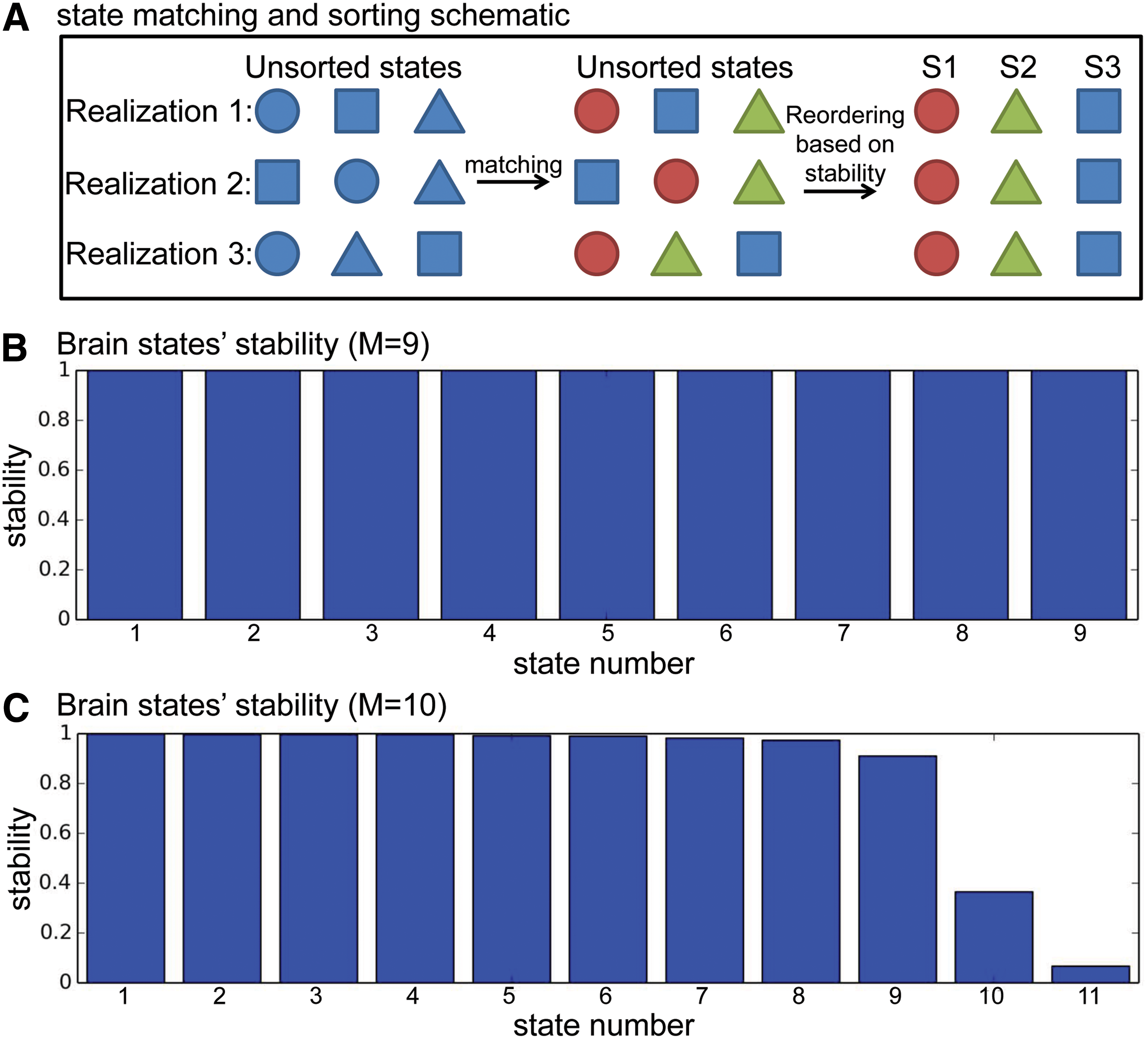
The schematic of state matching and sorting (A) and the resulting stability of each brain state when the total number of states is set to 9 (B), 10 (C). A toy example of the schematic of the state matching and sorting method with three states and three realizations is shown in (A). Spatial patterns of the brain states and the matched groups are represented by shapes and colors, respectively. The stability of brain states for M = 9 and M = 10 is shown in (B) and (C). Note that when M = 9, brain states from all the realizations are matched perfectly into 9 groups, while when M = 10, they are not matched perfectly, but grouped into 11 groups instead. Color images available online at www.liebertpub.com/brain

To test the reproducibility of our model on different datasets, we split the data of 100 subjects into two nonoverlapping groups of subjects (50 subjects each), and each half of the dataset was analyzed with the GHMM. The brain states extracted from both halves were compared to see whether the brain states were reproducible in different groups of subjects. Based on our results, we were able to find nine stable and highly reproducible brain states. Therefore, we subsequently set the total number of states to 9 when applying GHMM to resting-state fMRI data.

Brain state sequence decoding

The Viterbi algorithm (Viterbi, 1967) was used to decode the optimal brain state sequence, \documentclass{aastex}\usepackage{amsbsy}\usepackage{amsfonts}\usepackage{amssymb}\usepackage{bm}\usepackage{mathrsfs}\usepackage{pifont}\usepackage{stmaryrd}\usepackage{textcomp}\usepackage{portland, xspace}\usepackage{amsmath, amsxtra}\pagestyle{empty}\DeclareMathSizes{10}{9}{7}{6}\begin{document}$$\{ q_t \} , \,t = 1 , 2 , \ldots , T ,$$ \end{document} and determine which state the brain is under at each time point for all the scans after obtaining the optimal parameter set \documentclass{aastex}\usepackage{amsbsy}\usepackage{amsfonts}\usepackage{amssymb}\usepackage{bm}\usepackage{mathrsfs}\usepackage{pifont}\usepackage{stmaryrd}\usepackage{textcomp}\usepackage{portland, xspace}\usepackage{amsmath, amsxtra}\pagestyle{empty}\DeclareMathSizes{10}{9}{7}{6}\begin{document}$$\tilde { \lambda}$$ \end{document} in equation (1). We also calculated the posterior probability, \documentclass{aastex}\usepackage{amsbsy}\usepackage{amsfonts}\usepackage{amssymb}\usepackage{bm}\usepackage{mathrsfs}\usepackage{pifont}\usepackage{stmaryrd}\usepackage{textcomp}\usepackage{portland, xspace}\usepackage{amsmath, amsxtra}\pagestyle{empty}\DeclareMathSizes{10}{9}{7}{6}\begin{document}$$P ( q_t \mid \textbf{\textit{O}} , \tilde { \lambda} ) , t = 1 , 2 , \ldots , T$$ \end{document} , of each brain state at all the time points (Rabiner, 1989).

Spontaneous brain activity pattern of each state

We decoded the hidden brain state sequence for all the subjects and realizations with the Viterbi algorithm. After matching and grouping the brain states of different realizations, a time frame was labeled with a state only when it was assigned to the same state in all the realizations. Then the Z-scores of all the time frames that have been under the same state were computed as a representation of the spontaneous brain activity pattern of the brain state.

Results

After grouping the brain states from all 10 realizations, the stability of brain states was calculated. The states were subsequently sorted in the order of descending stability (S1 is defined to be the most stable state). Figure 2B and C show the stability of the resultant brain states when the total number of states, M, was set to 9 and 10, respectively. When M = 9, each of the nine states was able to match to a corresponding state in all 10 realizations, and thus only nine groups emerged (Fig. 2B). However, when M = 10, some states in some realizations failed to find a match in other realizations, so there were 11 possible groups for this case (Fig. 2C). Figure 2B and C illustrate that the stabilities of brain states are close to 1 when the total number of states is 9, whereas some states start to exhibit low stabilities when the total number of states is set to 10. In fact, with varying number of states (M = 5, 8, 9, 10, 11, 12, 20), it was found that the stabilities are almost 1 when M is set to 9 or less, but substantially less than 1 when M is greater than 9. Therefore, for the subsequent analysis, the number of states was set to 9.

The brain states detected from the nonoverlapping split-half samples of subjects are presented in Figure 3. The nine brain states extracted from the entire group of 100 subjects and two nonoverlapping samples of 50 subjects are almost identical (Fig. 3A). As can be seen in Figure 3B, correlation coefficients between the brain states from the two halves of the dataset indicate that the spatial patterns of all brain states are highly reproducible across different groups of subjects (p << 0.001). Although the correlation coefficient of the last state is the lowest, it is still statistically significant (p << 0.001). The last state also has relatively low Z-scores (darker colors in Fig. 3A and no patterns after thresholding in Fig. 4) compared to the other eight states. The spatial patterns of the nine stable and highly reproducible brain states detected from the entire dataset, denoted as S1 to S9, are further demonstrated in Figure 4. For better visualization, Figure 4 only displays Z-scores below −20 or above 20. For each state, a brain region with large positive or negative Z-scores indicates that it is highly activated or deactivated. Note that the absolute Z-scores in S9 are below 20 so no activation is seen in Figure 4 for S9.

FIG. 3.

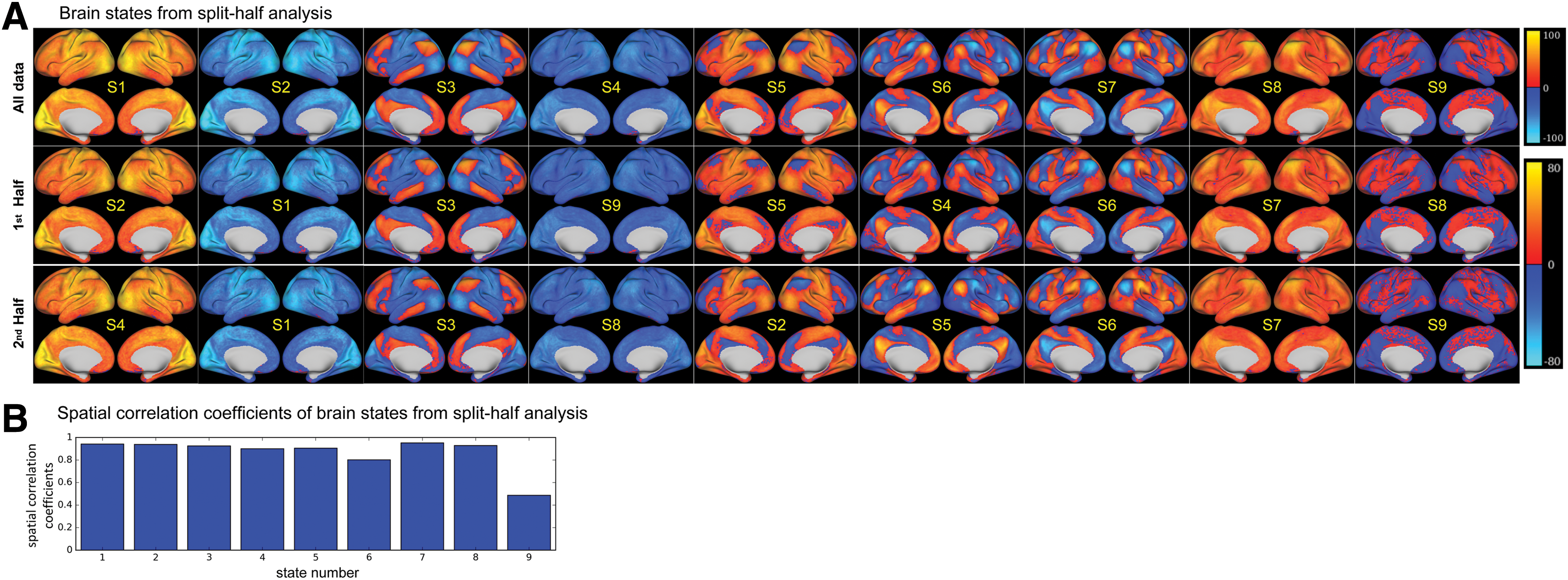
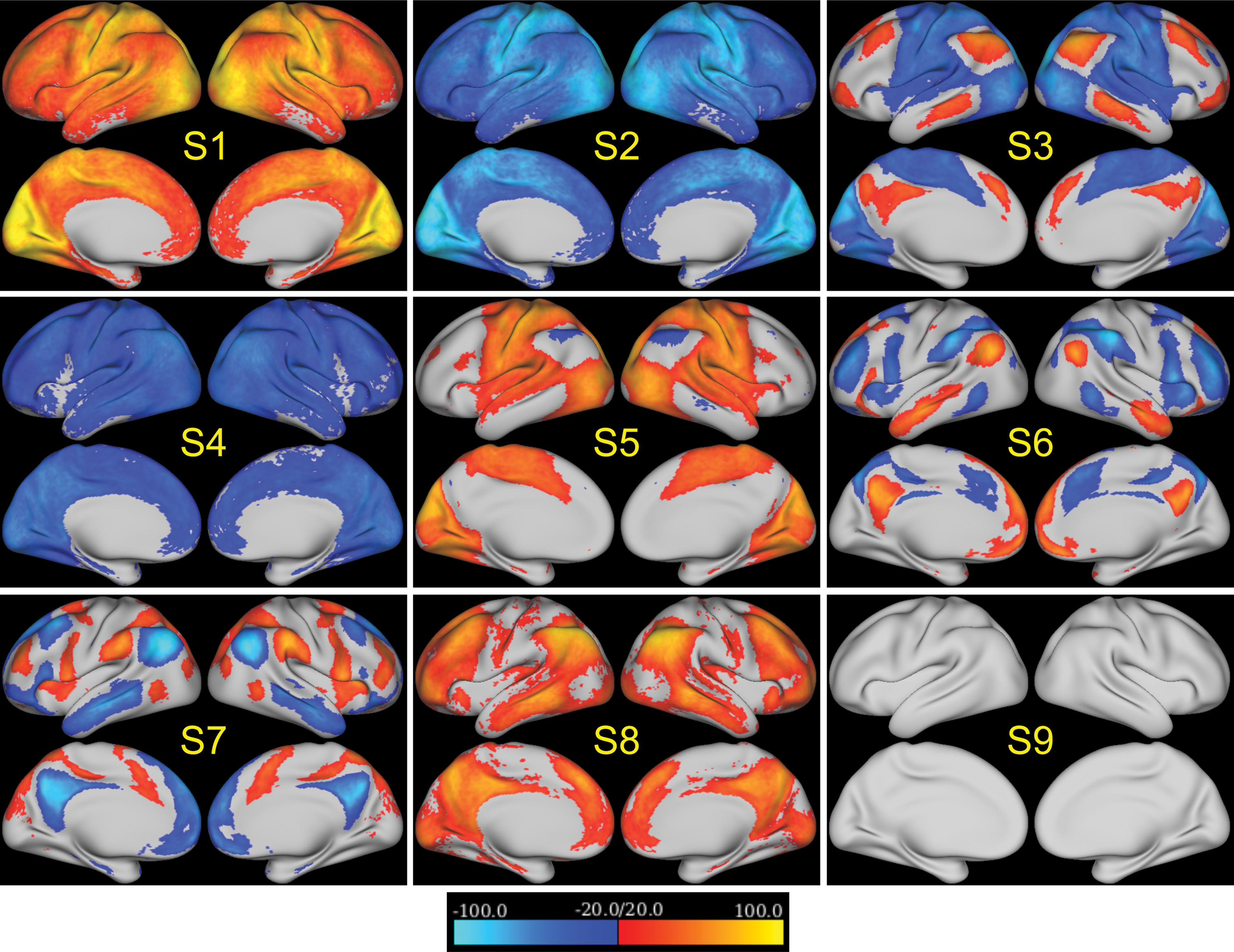
The reproducibility of brain states for split-half samples. (A) The Z-map of brain states detected from all 100 subjects and two nonoverlapping halves of the dataset. States with similar spatial patterns are aligned in the same column. (B) The spatial correlation coefficients of two states from the two halves are plotted to show the similarity between them. Note that the last state has the lowest spatial similarity and the lowest Z-score on its Z-map. Color images available online at www.liebertpub.com/brain

FIG. 4.

The Z-maps of nine reproducible brain states. The color bar is set to only display Z-scores below −20 or above 20. These brain states are different combinations of activated and deactivated brain regions. Color images available online at www.liebertpub.com/brain

All detected brain states consist of combinations of activated and deactivated brain regions. For example, as shown in Figure 4, brain activities in S6 and S7 are concentrated in regions specific to default mode and attention networks. S6 contains activation in the DMN and deactivation in the attention network, whereas S7 is comprised of deactivation in the DMN and activation in the attention network. Brain states S3 and S5 are almost opposite in a sense that S5 is comprised of activation in the sensorimotor and visual networks along with deactivation in the frontoparietal control network, while S3 contains deactivation in the sensorimotor and visual networks plus activation in the frontoparietal control network and DMN. Meanwhile, S1 and S2 are whole brain activation or deactivation with sensorimotor and visual networks being the most activated or deactivated. Also, S8 and S4 show whole brain activation and deactivation, but with lower intensities than those in S1 and S2. The final state, S9, has less apparent activation or deactivation patterns in known networks compared with other states.

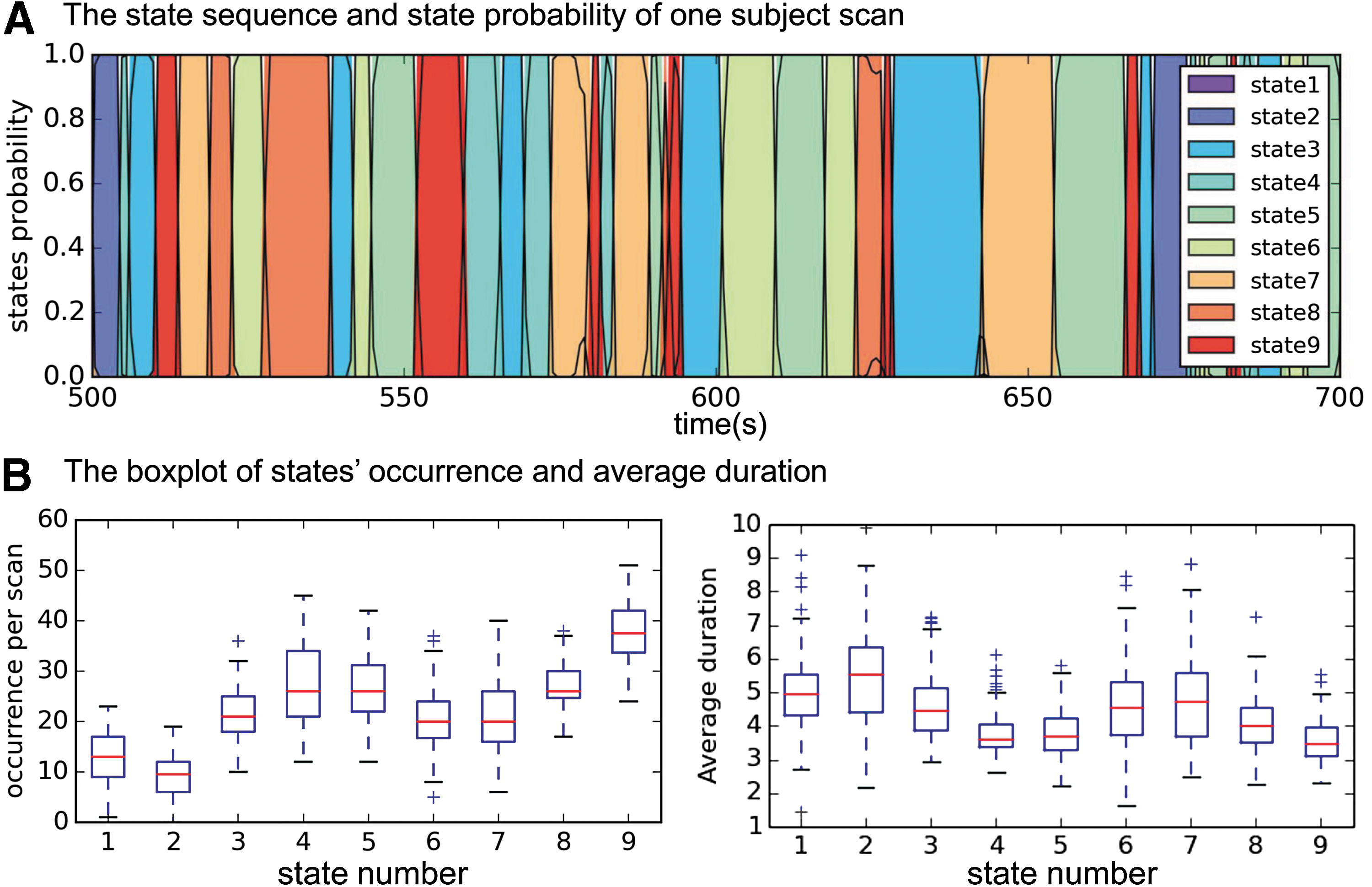
We also found that the brain is constantly switching among different states. Figure 5A shows an example of a sequence of brain states and how the posterior probability, \documentclass{aastex}\usepackage{amsbsy}\usepackage{amsfonts}\usepackage{amssymb}\usepackage{bm}\usepackage{mathrsfs}\usepackage{pifont}\usepackage{stmaryrd}\usepackage{textcomp}\usepackage{portland, xspace}\usepackage{amsmath, amsxtra}\pagestyle{empty}\DeclareMathSizes{10}{9}{7}{6}\begin{document}$$P ( q_t \mid \textbf{\textit{O}}_{\textbf{\textit{t}}} , \tilde{ \lambda} )$$ \end{document} , of each state changes over time. In Figure 5A, the state sequence decoded by the Viterbi algorithm is represented by different colors, while the posterior probability is plotted with black curves. Figure 5B illustrates the occurrence and average duration of each state. Note that S9 occurs most frequently while S1 and S2 occur less frequently.

FIG. 5.

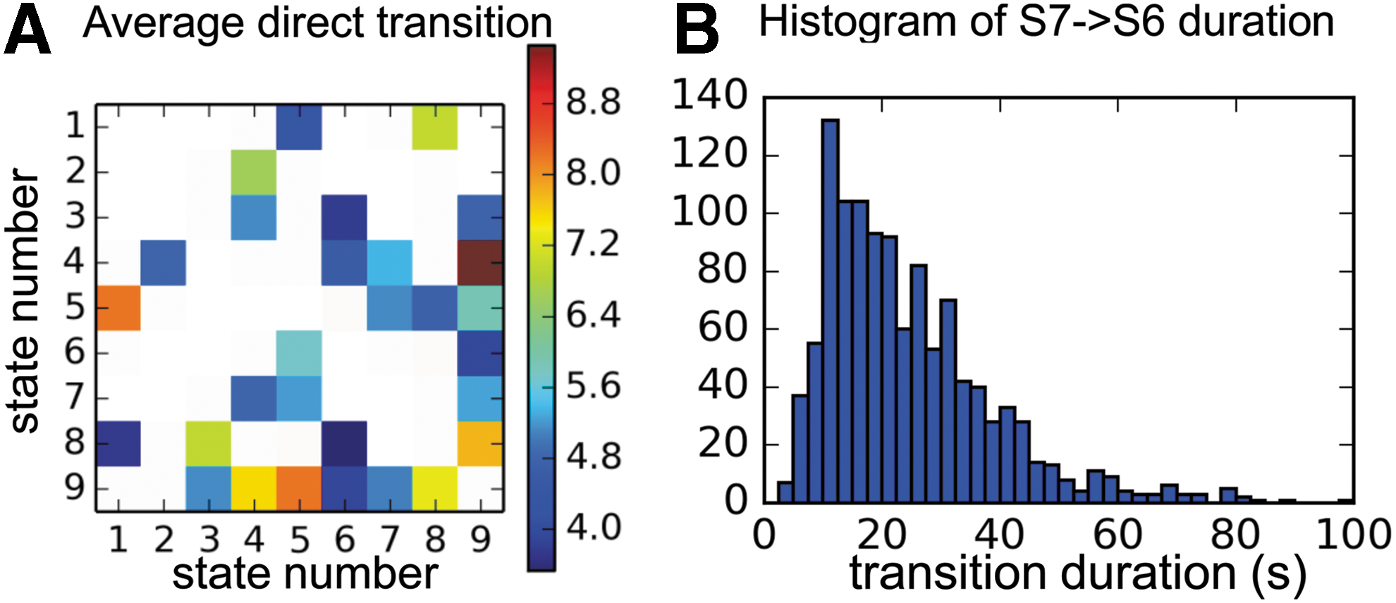
Temporal characteristics of the brain state. (A) The state sequence and state probability during one subject scan. Only a period of the scan is demonstrated in the figure for better visualization. Different colors indicate what the subject's brain state is at each time point. The black curves are the posterior probability of different brain states. (B) Boxplots of states' occurrence and average duration. Note that the length of each scan is 14.4 min. Color images available online at www.liebertpub.com/brain

After decoding the state sequence, we counted the number of transitions between states and calculated the average direct transition times between each pair of states. Only transitions that are significantly more frequent than the average are color coded in Figure 6A (p < 0.0007. Since this is a multiple comparison, Bonferroni correction has been applied to the α value). Note that most of the states (except S1 and S2) transit to S9 frequently, and S9 also switches back to other states frequently.

FIG. 6.

The transition properties of the brain states. (A) Average direct transition per scan. Note that only when the transition times from state i to state j is significantly higher than average (p < 0.0007), the block in the ith row and jth column will be color coded. (B) Histogram of the duration of the motif from the beginning of S7 to the end of S6. Color images available online at www.liebertpub.com/brain

The transition from the DMN activation to the attention network activation has been noted previously (Majeed et al., 2011). Based on our results, S7 shows attention network activation, whereas S6 exhibits DMN activation. Therefore, we investigated the duration of the motif from the beginning of S7 to the end of S6 (direct and indirect transitions have both been accounted for). Figure 6B shows the histogram of the duration, in which the peak of the distribution lies between 10 and 20 seconds.

To illustrate the advantage of exploiting temporal information, the method used in CAPs (Liu et al., 2013; Liu and Duyn, 2013), k-means, was applied on the signal from the 236 ROIs used in the GHMM analysis. For this analysis, the split-half approach described in the Materials and Methods section was repeated and the reproducibility of the states derived with the repeated application of k-means was tested. For comparison, the number of initializations and repetitions used was identical to that for the GHMM analysis. Supplementary Figure S1 (Supplementary Data are available online at www.liebertpub.com/brain) shows the spatial patterns of resultant cluster centers, which are denoted by C1 to C9. Note that for most of the states derived by GHMM (S1, S2, S3, S5, S6, and S8), we can find very similar patterns in these cluster centers derived by k-means, while whole brain deactivation (S4) and attention networks (S7), and their corresponding cluster centers (C1 and C8) have relatively low spatial correlation coefficients. No spatial patterns similar to S9 can be found in these cluster centers (Supplementary Fig. S1C and Fig. 3). Moreover, the reproducibility of C5 and C7 are relatively low compared to the rest (Supplementary Fig. S1B).

Discussion

In general, the Markov property can be applied on either temporal or spatial axes of data. When it is used to model spatial relationship among voxels, it is called a Markov random field and a binary state switch is typically assumed for each voxel (Lindquist et al., 2007; Liu et al., 2014; Robinson et al., 2010). When the Markov property is assumed on the temporal axis, it is a Markov random process and has been employed to investigate variability in functional connectivity over time (Eavani et al., 2013; Ou et al., 2014). In contrast to the previous application of HMM, we applied the GHMM on temporal axis to model the spontaneous brain activity state switching process. Moreover, we introduced a robust approach for determining the number of states based on the stability. The nonstationary assumption of the GHMM provides the ability to capture the dynamics of the brain activity measured by the resting-state fMRI. Our spatiotemporal model of spontaneous activities across the brain in resting-state fMRI was able to identify nine stable brain states with reproducibility near 1. Furthermore, the detected brain states have analogues to combinations of conventional resting-state networks (RSNs). The implications of these results are discussed in the following paragraphs.

The reproducibility of GHMM on estimating brain states is affected by two factors: (1) algorithmic stability and (2) the dataset that the model is trained on. Since the algorithm is nonconvex, there is no guarantee of a global optimum and different initializations can lead to different local optima. Increasing the repetitions of the algorithm with different initializations will increase the chance for the algorithm to reach the global optimum and, thus, increase the stability of the results. Increasing the total number of states will increase the number of parameters in the model, which may lead to a more complicated model with more local optima and thus a less stable result. This could explain the low stability of some states when the total number of states is larger than 9 (Fig. 2C). Meanwhile, different datasets, O , will result in different objective functions, P( O |λ), and thus different best-fitting model parameters λ. This is due to the fact that subjects in different fMRI scans may experience different brain states. Our results (Figs. 2 and 3) show that brain states detected by GHMM are both stable and reproducible on different datasets, indicating that the model is able to extract the common features within this group of subjects. The stabilities of all nine states are almost 1, as shown in Figure 2B, indicating the brain states from all realizations are very similar and can be matched perfectly into nine groups. Therefore, changing the threshold, 0.8, to a higher value, when matching states, will not lead to any differences in the final results. Moreover, when comparing the reproducibility of the cluster centers derived by k-means and our model (Supplementary Fig. S1B), the higher reproducibility of our result (Fig. 3B) is due to additional temporal information included in our model.

No spatial constraint is imposed in our GHMM, yet the nine states identified exhibit smooth contiguous activated and deactivated regions. We further note that these activated and deactivated brain regions resemble conventional RSNs. For example, the whole brain deactivation states, S2 and S4, have been found by temporal functional modes (Smith et al., 2012). Also, linear combinations of activated/deactivated DMN and deactivated/activated attention network, S6 and S7 (Fig. 4), have also been reported as CAPs (Liu et al., 2013; Liu and Duyn, 2013). The existence of these two brain states explains why DMN and attention network are often anticorrelated in seed-based correlation analysis (Fox et al., 2006). Our results further indicate that these two networks are only anticorrelated when the brain is in S6 and S7, rather than during the entire scan. Moreover, the switch between different states leads to changing correlation and anticorrelation patterns and, thus, can explain why the functional connectivity changes over time (Allen et al., 2014). Comparing Figure 3 and Supplementary Figure S1A, we note that most of the spatial patterns of brain states detected by our GHMM (S1, S2, S3, S5, S6, and S8) are similar to those detected by k-means (Supplementary Fig. S1C), indicating that most of our brain states are consistent with those detected by CAPs.

As shown in Figure 5, the duration of states differs for each state and even differs for each occurrence. Therefore, the use of conventional sliding window-based analysis with fixed window length can lead to signals from multiple brain states being merged together and possibly canceling each other. Based on our results, we recommend decoding the brain state sequence first and then determining the window length according to the duration of states rather than fixing the length and sliding the window.

To the best of our knowledge, a state similar to S9 has not been presented in previous literature. We hypothesize that S9 is the “ground” state of the brain, in which brain activity (or deactivity) is similar for the entire cortex (no apparent activation or deactivation as shown in Fig. 4). Note that different groups of subjects have different spatial patterns for state S9 (Fig. 3A). Therefore, S9 has the lowest reproducible spatial pattern (Fig. 3B). However, its temporal characteristics allowed us to distinguish it consistently from other states. S9 occurs more frequently (37.5 ± 6.4 times per scan. or per 14.4 min) compared to other brain states and has a short duration (3.6 ± 0.6 sec; Fig. 5B). From the transition matrix in Figure 6A, we can see that most states (except S1 and S2) often switch to S9 and then transit back to other states from S9. The spatial and temporal characteristics of S9 indicate that it is an intermediate transient state that appears when the brain is switching between other more reproducible brain states and could represent a “ground” state. Note that the low reproducibility of S9's spatial pattern makes it difficult to detect using methods that only consider spatial information when defining states. This may be the reason why k-means cannot detect this state (Supplementary Fig. S1A). Our ability to detect it could be due to the additional temporal information inherent in our model.

States S7 and S6 have similar spatial activation patterns as the attention network and DMN, respectively, reported in literature (Broyd et al., 2009; Buckner et al., 2008) (Supplementary Fig. S2). Prior work (Majeed et al., 2011) found a reproducible transition from activation in attention network (similar to S7) to activation in DMN (similar to S6) within a 20 sec sliding window. Interestingly, the present method also detected similar transition duration between these states. The histogram of the motif from the beginning of S7 to the end of S6 in Figure 6B shows that there exists a peak between 10 and 20 sec, indicating that the motif is more likely 10 to 20 sec in duration, consistent with what was reported in the literature (Majeed et al., 2011). Note that this transition from S7 to S6 not only accounts for direct transition, but also includes indirect transitions through intermediate states (e.g., S7->S9->S6), which were also shown by Majeed and coworkers (2011).

The intrinsic advantage of GHMM over CAPs is that GHMM quantifies state transitions explicitly using a Markov chain in the model. The quantification of state transition not only provides the ability to capture temporal characteristics (Figs. 5 and 6), but also give rise to additional brain states. Specifically, the 9th state, detected by GHMM, due to a relatively low reproducibility of its spatial pattern, is difficult to capture by methods that only consider spatial similarity, such as k-means used by CAPs. However, since S9 has distinctive temporal properties (high occurrence frequency and short duration), GHMM is able to detect it consistently (Fig. 3). Supplementary Figure S1C further illustrates that there are spatial differences in activation patterns between CAPs and GHMM in other brain states as well, including the whole brain deactivation (C1 for CAPs and S4 for GHMM) and attention networks (C8 for CAPs and S7 for GHMM).

The results in this work must be considered in the context of several limitations. First, we assume a memory-less transition between brain states by using Markov chains, that is, the current brain state only depends on the previous state. Fortunately, the HMM is robust to violations of this assumption and has been successfully applied to speech recognition (Rabiner, 1989) as well as detection of brain states from electrophysiological measurements (Jones et al., 2007), neither of which is a memory-less system. Another methodological limitation is that state duration is not modeled explicitly in the present work, and to stay in the same state, the system needs to conduct a self-transition, which would decrease the probability of staying in the same state exponentially over time. In future work, the HMM with explicit duration can be applied, and the duration probability distribution will be trained with the dataset as well. Due to computational limitations, we only trained our GHMM with 236 time courses from the brain of each subject. A voxel-wise GHMM may be able to capture more detailed spatial characteristics of the states. In the present work, we have applied temporal filtering (0.01–0.1 Hz) to focus on the low frequency spontaneous activity (Fox et al., 2005). However, recent studies have demonstrated that visual and sensorimotor networks are also present in higher frequencies (0.5–0.8 Hz) (Lee et al., 2013). We plan to study the effect of different temporal resolutions by applying GHMM to high temporal resolution data and study brain state switching process at other time scales.

Conclusion

We have applied GHMM to analyze resting-state fMRI. The GHMMs the brain state switching process as a Markov chain and the brain states as multivariate Gaussian distribution. Spatially, nine stable and reproducible brain states were discovered and found to be combinations of activated or deactivated RSNs. Temporally, we were able to derive the brain state sequence for individual subjects with the model, and evaluate the occurrence and duration of each state. One transient state, S9, was identified based on its spatiotemporal characteristics. The motif from activated attention network (S7) to activated DMN (S6) was also found to be consistent with previous literature. Therefore, we conclude that the study of brain state sequential switching process can unveil spatiotemporal pattern of the brain and further improve our understanding of brain dynamics.

Footnotes

Acknowledgments

The authors thank Jaemin Shin for his useful suggestions. This work was supported in part by the Georgia Research Alliance.

Author Disclosure Statement

No competing financial interests exist.

References

Allen

, Damaraju

, Plis

, Erhardt

, Eichele

, Calhoun

. 2014. Tracking whole-brain connectivity dynamics in the resting state. Cereb Cortex, 24:663–676.

Baker

, Brookes

, Rezek

, Smith

, Behrens

, Smith

PJP

, Woolrich

. 2014. Fast transient networks in spontaneous human brain activity. Elife, 3:e01867.

Beckmann

, DeLuca

, Devlin

, Smith

. 2005. Investigations into resting-state connectivity using independent component analysis. Philos Trans R Soc Lond B Biol Sci, 360:1001–1013.

Bilmes

. 1998. A gentle tutorial of the EM algorithm and its application to parameter estimation for Gaussian mixture and hidden Markov models. Int Comput Sci Inst, 4:126.

Broyd

, Demanuele

, Debener

, Helps

, James

, Sonuga-Barke

. 2009. Default-mode brain dysfunction in mental disorders: a systematic review. Neurosci Biobehav Rev, 33:279–296.

Buckner

, Andrews‐Hanna

, Schacter

. 2008. The brain's default network. Ann N Y Acad Sci, 1124:1–38.

Eavani

, Satterthwaite

, Gur

, Davatzikos

. 2013. Unsupervised learning of functional network dynamics in resting state fMRI. Inf Proce Med Imaging, 23:426–437.

Eddy

. 1996. Hidden markov models. Curr Opin Struct Biol, 6:361–365.

Fox

, Corbetta

, Snyder

, Vincent

, Raichle

. 2006. Spontaneous neuronal activity distinguishes human dorsal and ventral attention systems. Proc Natl Acad Sci U S A, 103:10046–10051.

10.

Fox

, Snyder

, Vincent

, Corbetta

, Van Essen

, Raichle

. 2005. The human brain is intrinsically organized into dynamic, anticorrelated functional networks. Proc Natl Acad Sci U S A, 102:9673–9678.

11.

Glasser

, Sotiropoulos

, Wilson

, Coalson

, Fischl

, Andersson

, Xu

, Jbabdi

, Webster

, Polimeni

. 2013. The minimal preprocessing pipelines for the Human Connectome Project. Neuroimage, 80:105–124.

12.

Griffanti

, Salimi-Khorshidi

, Beckmann

, Auerbach

, Douaud

, Sexton

, Zsoldos

, Ebmeier

, Filippini

, Mackay

. 2014. ICA-based artefact removal and accelerated fMRI acquisition for improved resting state network imaging. Neuroimage, 95:32–247.

13.

Hanke

, Halchenko

, Sederberg

, Hanson

, Haxby

, Pollmann

. 2009. PyMVPA: a python toolbox for multivariate pattern analysis of fMRI data. Neuroinformatics, 7:37–53.

14.

Jones

, Fontanini

, Sadacca

, Miller

, Katz

. 2007. Natural stimuli evoke dynamic sequences of states in sensory cortical ensembles. Proc Natl Acad Sci U S A, 104:18772–18777.

15.

Keilholz

. 2014. The neural basis of time-varying resting-state functional connectivity. Brain Connect, 4:769–779.

16.

Lee

H-L

, Zahneisen

, Hugger

, LeVan

, Hennig

. 2013. Tracking dynamic resting-state networks at higher frequencies using MR-encephalography. Neuroimage, 65:216–222.

17.

Lindquist

, Waugh

, Wager

. 2007. Modeling state-related fMRI activity using change-point theory. Neuroimage, 35:1125–1141.

18.

Liu

, Awate

, Anderson

, Fletcher

. 2014. A functional network estimation method of resting-state fMRI using a hierarchical Markov random field. NeuroImage, 100:520–534.

19.

Liu

, Chang

, Duyn

. 2013. Decomposition of spontaneous brain activity into distinct fMRI co-activation patterns. Front Syst Neurosci, 7:101.

20.

Liu

, Duyn

. 2013. Time-varying functional network information extracted from brief instances of spontaneous brain activity. Proc Natl Acad Sci U S A, 110:4392–4397.

21.

Majeed

, Magnuson

, Hasenkamp

, Schwarb

, Schumacher

, Barsalou

, Keilholz

. 2011. Spatiotemporal dynamics of low frequency BOLD fluctuations in rats and humans. Neuroimage, 54:1140–1150.

22.

, Xie

, Jin

, Li

, Zhu

, Jiang

, Chen

, Zhang

, Li

, Liu

. 2014. Characterizing and differentiating brain state dynamics via hidden Markov models. Brain Topogr, 28:666–679.

23.

Pedregosa

, Varoquaux

, Gramfort

, Michel

, Thirion

, Grisel

, Blondel

, Prettenhofer

, Weiss

, Dubourg

. 2011. Scikit-learn: machine learning in Python. J Mach Learn Res, 12:2825–2830.

24.

Power

, Cohen

, Nelson

, Wig

, Barnes

, Church

, Vogel

, Laumann

, Miezin

, Schlaggar

. 2011. Functional network organization of the human brain. Neuron, 72:665–678.

25.

Rabiner

. 1989. A tutorial on hidden Markov models and selected applications in speech recognition. Proc IEEE, 77:257–286.

26.

Rabinovich

, Muezzinoglu

. 2010. Nonlinear dynamics of the brain: emotion and cognition. Phys Usp, 53:357.

27.

Robinson

, Wager

, Lindquist

. 2010. Change point estimation in multi-subject fMRI studies. Neuroimage, 49:1581–1592.

28.

Sakoğlu

, Pearlson

, Kiehl

, Wang

, Michael

, Calhoun

. 2010. A method for evaluating dynamic functional network connectivity and task-modulation: application to schizophrenia. Magn Reson Mater Phys Biol Med, 23:351–366.

29.

Salimi-Khorshidi

, Douaud

, Beckmann

, Glasser

, Griffanti

, Smith

. 2014. Automatic denoising of functional MRI data: combining independent component analysis and hierarchical fusion of classifiers. Neuroimage, 90:449–468.

30.

Smith

, Miller

, Moeller

, Xu

, Auerbach

, Woolrich

, Beckmann

, Jenkinson

, Andersson

, Glasser

. 2012. Temporally-independent functional modes of spontaneous brain activity. Proc Natl Acad Sci U S A, 109:3131–3136.

31.

Van Essen

, Glasser

, Dierker

, Harwell

, Coalson

. 2012. Parcellations and hemispheric asymmetries of human cerebral cortex analyzed on surface-based atlases. Cereb Cortex, 22:2241–2262.

32.

Van Essen

, Smith

, Barch

, Behrens

, Yacoub

, Ugurbil

, and Wu-Minn

HCP

. Consortium. 2013. The WU-Minn Human Connectome Project: an overview. Neuroimage, 80:62–79.

33.

Viterbi

. 1967. Error bounds for convolutional codes and an asymptotically optimum decoding algorithm. Inform Theory IEEE Trans, 13:260–269.

34.

Yang

, LaConte

, Weng

, Hu

. 2008. Ranking and averaging independent component analysis by reproducibility (RAICAR). Hum Brain Mapp, 29:711–725.

Supplementary Material

Please find the following supplemental material available below.

For Open Access articles published under a Creative Commons License, all supplemental material carries the same license as the article it is associated with.

For non-Open Access articles published, all supplemental material carries a non-exclusive license, and permission requests for re-use of supplemental material or any part of supplemental material shall be sent directly to the copyright owner as specified in the copyright notice associated with the article.

0.00 MB

0.29 MB

0.27 MB