
Abstract
The relationship between structural and functional brain networks is still highly debated. Most previous studies have used a single functional imaging modality to analyze this relationship. In this work, we use multimodal data, from functional MRI, magnetoencephalography, and diffusion tensor imaging, and assume that there exists a mapping between the connectivity matrices of the resting-state functional and structural networks. We investigate this mapping employing group averaged as well as individual data. We indeed find a significantly high goodness of fit level for this structure–function mapping. Our analysis suggests that a functional connection is shaped by all walks up to the diameter in the structural network in both modality cases. When analyzing the inverse mapping, from function to structure, longer walks in the functional network also seem to possess minor influence on the structural connection strengths. Even though similar overall properties for the structure–function mapping are found for different functional modalities, our results indicate that the structure–function relationship is modality dependent.
Introduction
Applying network science has become a common practice in neuroscience to understand functional interactions in the healthy brain and identify abnormalities in brain disorders (Stam, 2014). The collection of these functional connections is often referred to as the functional network and is facilitated by the underlying structural network, that is, the set of physical connections between neuronal populations. At the same time, functional connections influence modulations of these physical connections by long-term potentiation, plasticity, or neuromodulation.
In recent years, there has been an increasing interest to understand the emergence of functional brain networks given the constraints of the underlying structural network (Abdelnour et al., 2014; Deco et al., 2012; Honey et al., 2009; Senden et al., 2014). However, the mutual relationship between the structural and functional networks remains highly debated (Deco et al., 2014; Robinson, 2012; Robinson et al., 2014).
Empirical studies have revealed an overlap between structural and (resting-state) functional connections, that is, the presence of both a structural and functional connection between two brain regions (Hermundstad et al., 2013; Skudlarski et al., 2008; van den Heuvel et al., 2009). However, this overlap is imperfect as functional interactions between brain regions exist in the absence of direct structural connections, and also, indirect structural connections with the length of two links cannot fully account for these functional connections either (Honey et al., 2009).
Moreover, the overlap between structural and functional connections also depends on the time scale considered, where functional connections estimated from larger time windows strongly overlap with the underlying structural connections, for smaller time windows there can be a structural–functional network discrepancy due to distributed delays between neuronal populations that cause transient phase (de-)synchronization (Honey et al., 2007; Messé et al., 2014; Ton et al., 2014).
On larger time scales, several properties of the underlying structural network have been shown to play an essential role in shaping the functional networks, such as the Euclidian distance between two brain regions (Alexander-Bloch et al., 2013). However, taking into account Euclidean distance alone is insufficient to explain the emergence of long-range functional connections (Vértes et al., 2012).
Two recent studies showed that such long-range functional connections may be explained by the product of the degree of two nodes in the structural network, indicating the crucial role of structural hubs for explaining long-range functional connections (Stam et al., 2015; Tewarie et al., 2014). Moreover, Goñi and colleagues (2014) demonstrated that shortest paths in the structural network and perturbations from these paths are strong predictors for functional connections as these paths are favorable because of metabolic efficiency and fast communication.
Given these dependencies between structural and functional networks, the challenge is to integrate these different interdependencies into a single framework, for which we may need a more abstract representation. For example, a significant overlap in the connectivity profile of structural and functional networks suggests that part of the functional network connectivity matrix is a linear mapping from its structural counterpart. In addition, functional connections can also be accounted for by several other higher order features of the structural network as outlined above, which refer to nonlinear relationships [see Tewarie et al. (2014) for an example of such nonlinearity].
Based on the presence of these linear and nonlinear features of the relationship between structural and functional networks, we go one step further by assuming that there is a mathematical function that maps the adjacency matrix of the structural network on that of the (resting-state) functional network and vice versa [see Fig. 1b and Eq. (1) below]. If we further assume that our mathematical function is analytic (Titchmarsh, 1939; Whittaker et al., 1996), then the map between structural and functional network can be expressed by a weighted sum of the matrix powers as explained in Mathematical Background section.
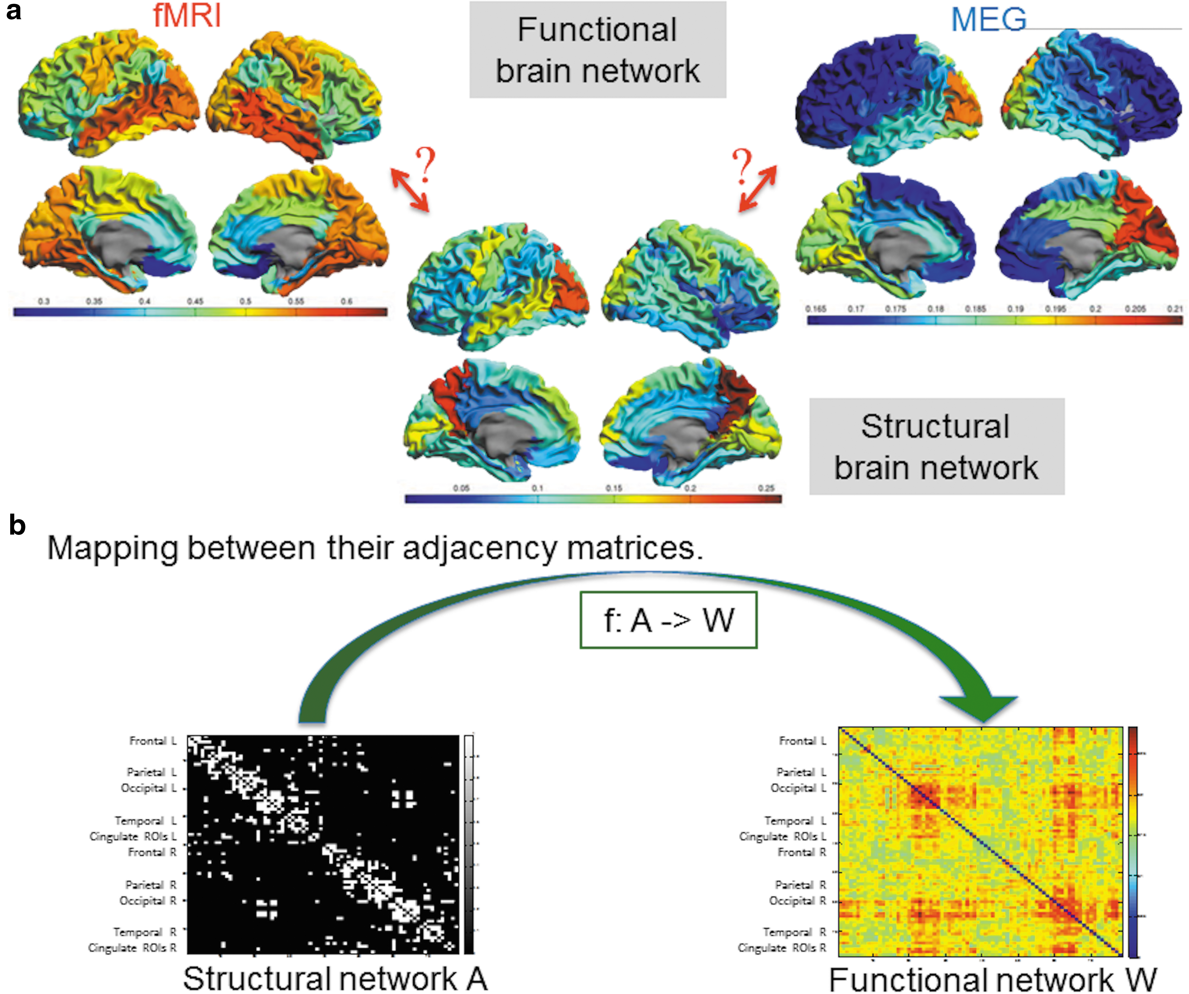
Our method consists of a data-driven approach, from which the successive coefficients of this matrix mapping are determined. The major advantage of our method is that an a-priori specific form of a function is not needed. Another implication of such a function is the possible existence of an inverse function, that is, a mapping from functional networks back to structural networks.
Most previous studies have found relationships between structural and functional networks using a single functional neuroimaging modality (Damoiseaux and Greicius, 2009; Honey et al., 2009), often using functional MRI (fMRI). As the fMRI response is an indirect measure for the neuronal activity and contains nonneuronal signals, a structure–function dependency based on this modality could deviate from the same dependency derived from neuroimaging modalities that directly measure the neuronal activity and connectivity. In contrast to fMRI, magnetoencephalography (MEG) measures the neuronal activity and connectivity directly with excellent temporal resolution.
However, given the increasing interest in multimodal imaging approaches, there is a need to understand the modality dependency of the structure–function relationship in a single framework. A data-driven approach in the form of a matrix function may be helpful when investigating the modality dependency of the structural–functional network relationship: different modality-dependent coefficients may point to different specific functions for each modality. The relevance of elucidating the modality dependency of a mathematical function can be extended to the clinical field where we could answer questions such as the following: which modality would be the most sensitive for picking up functional network changes given disease-specific structural network damage?
The aim of this study is to analyze the structural–functional network relationship through a mathematical function in a multimodal framework. We use two datasets containing multimodal imaging data ranging from diffusion tensor imaging (DTI) data to MEG and fMRI data. We extend our analysis by also considering the relationship between structural and functional networks at the subject level in a third data set and finally discuss how that relationship can be interpreted neurobiologically.
Materials and Methods
Participants and data acquisition
In total, we use three data sets, which have been used in different previous studies. The first two data sets are group-averaged data sets, obtained from two different centers, but analyzed together in one mapping.
(i) A group-averaged structural imaging data set, that is, a DTI network from 80 healthy subjects in 78 cortical automated anatomical labeling (AAL) brain areas (Gong et al., 2009).
(ii) Two group-averaged data sets with functional imaging data, that is, resting-state MEG and fMRI signals in the same 78 AAL cortical areas, one with 17 and another with 21 healthy subjects (Tewarie et al., 2014, 2015).
(iii) An individual data set from 11 healthy subjects' structural and functional imaging data, that is, with DTI, resting-state MEG, and fMRI time courses in 219 brain areas (Douw et al., 2015).
For the group-averaged structural connectivity matrix, we use a literature-based structural network [data set (i)] (Gong et al., 2009). In every subject, cortical regions in the AAL atlas were considered to be connected if the end-points of two white matter tracts were located in these regions (Gong et al., 2009). Then, a group-averaged structural connectivity matrix was obtained by testing each possible connection for its significance using a nonparametric sign test.
For the group-averaged functional imaging data set [data set (ii)], we use data obtained from our own imaging center. We employ the first data set with 17 healthy controls for our main analysis and the second data set from 21 healthy controls only for validation (Tewarie et al., 2014, 2015). The study was approved by the institutional ethics review board of the VUmc and all subjects gave written informed consent before participation. Both fMRI and MEG data sets underwent to some extent different pipelines (Tewarie et al., 2014, 2015) and are obtained from two different MEG scanners (CTF and Elekta). Detailed information about data acquisition and postprocessing can be found in the previous articles.
In short, for both MEG and fMRI, cortical networks were constructed using the same cortical AAL regions as for the structural network consisting of 78 cortical regions (Gong et al., 2009). The Pearson correlation coefficient was computed between time signals to construct functional networks for fMRI for each subject (the absolute value was taken to avoid negative matrix elements).
For MEG, a beamformer approach was used to reconstruct the neuronal activity in AAL regions. Subsequently, the phase lag index (PLI), a measure for phase synchronization, was computed between time series to reconstruct a functional connectivity matrix for each subject in the alpha2 frequency band (10–13 Hz) (Stam et al., 2007). This study can be considered a continuation from previous work where we found a strong relationship between structural and functional networks in the alpha2 band, and therefore, we limited our analysis to this frequency band, although the fit could be generalized (Tewarie et al., 2014).
Similar to the structural connectivity matrix, we averaged functional connectivity matrices across subjects for fMRI and MEG separately to obtain one group-averaged functional connectivity matrix for each modality. The averaging over multiple subjects was pursued in the attempt of reducing noise.
For the individual data set [data set (iii)], eleven healthy participants were included, exclusion criteria being psychiatric or neurological disease and use of medication influencing the central nervous system. This study was approved by MGHs institutional review board, and was performed in accordance with the Declaration of Helsinki. All participants gave written informed consent before participation. Preprocessing methodology of the DTI and fMRI data has been described in detail before (Douw et al., 2015). In short, a surface-based atlas approach was used for connectivity analysis of the fMRI and DTI data, using a parcellation scheme with 219 cortical surface parcels (Daducci et al., 2012; Gerhard et al., 2011). In addition, for every entry of the fMRI-based adjacency matrix, the absolute value was taken to avoid negative matrix elements.
MEG eyes-open resting-state data were collected in a magnetically shielded room with a 306-channel whole-head system (Elekta-Neuromag) and a sampling rate at 1037 Hz. Vertical and horizontal electrooculograms were acquired simultaneously for off-line eye-movement artifact rejection. Head positions relative to the MEG sensors were recorded from four head-position indicator coils attached to the scalp. Landmark points of the head were digitized using a 3D digitizer (Polhemus FASTRAK). MEG data underwent a number of preprocessing steps: (1) bad channel and bad epoch rejection, (2) eye-movement artifact removal by Signal Space Projection, (3) downsampling with a decimate factor of 8 (to reduce computational expense).
To compute the physical forward solution (lead fields), a single-layer boundary element method was applied to model the brain volume conduction, following an established procedure (Hämäläinen and Sarvas, 1987). The lead field of freely oriented dipoles was then evaluated at each location. In solving the inverse problem, current density at each source location was approximated by a minimum two-norm estimate in the same six frequency bands as was used for the second dataset (Hämäläinen and Ilmoniemi, 1994), with noise covariance computed from empty-room recordings on the same day (also band-pass filtered).
For each subject, the cortical surface defined by the boundary between the gray and the white matter was reconstructed using FreeSurfer (Fischl et al., 1999), after which time series from the above-mentioned 219 cortical surface parcels were reconstructed. The PLI was used as a connectivity measure on these time series (Stam et al., 2007). An average connectivity matrix per participant was calculated over all epochs.
Mathematical background
We will refer to matrix A as the binary adjacency matrix of the structural network for the group-averaged data [data set (i)] and to matrix W as one of the possible representations of the functional networks, W MEG for MEG functional networks and W fMRI for fMRI functional networks. Both A and W are N × N symmetric matrices, where N equals the number of cortical regions [N = 78 for data set (i) and (ii); N = 219 for data set (iii)]. For both group-averaged and individual data, the matrix W has real elements w ij between 0 and 1. In the case of the individual data, the structural network is described by a weighted adjacency matrix V with real elements between 0 and 1.
As mentioned before, we assume that there exists a function f such that
or W = f(V) in the case of a weighted structural connectivity matrix V (see also Fig. 1). Under quite mild conditions (Markushevich, 1985), the inverse f
−1 of the function f exists such that
If f(z) is a function of the complex number z and analytic in a disk with radius R around z
0, then f(z) possesses a Taylor series in the complex plane ℂ that converges for all points z that lie in a disk with radius R around the point
where |z − z
0| < R and R is called the radius of convergence (Titchmarsh, 1939; Whittaker et al., 1996). It can be shown (Higham, 2008; Van Mieghem, 2011) that, if f(z) is analytic around z
0 and, hence, possesses a Taylor series Eq. (3), then for all matrices A, the matrix function f(A) also satisfies this Taylor series, provided each eigenvalue λ of A obeys |λ−z
0| < R. Caley-Hamilton's famous theorem (Van Mieghem, 2011) states that any square matrix A satisfies its own characteristic polynomial, which implies that we can write
shows that
where c k[f] are coefficients depending on the function f (provided each eigenvalue λ of A lies within the disk, that is, obeys |λ−z 0| < R). Because all the analyzed matrices have only zeros on the diagonal, their trace is 0. Since the trace equals the sum of the eigenvalues of a matrix (Van Mieghem, 2011), the average of the eigenvalues of the empirical matrices here is zero, which suggests us to choose z 0 = 0.
Mathematical methodology
The first term
where K ≤ N − 1 is the maximal fitted exponent (N is the dimension of matrix A). We use the nonlinear regression algorithm in MATLAB (using the routine nlinfit.m version R2015a) to estimate the coefficients in Eq. (5) by iterative least-squares estimation (for details see Supplementary Information [SI]-H; Supplementary Data are available online at
Denoting
where N = 78 regions in the case of the group-averaged data and N = 219 in the case of the individual data. In this study, we only sum the elements of the lower triangular and the diagonal because all our matrices are symmetric. Since the SSEs is proportional to the number of fitted elements and to compare the different data sets with each other, we introduce a normalized version of SSE where we divide SSE by the degrees of freedom, which is in our case the number of fitted elements minus one
where df top = N*(N − 1)/2 + N − 1, N number of regions. Similarly, we can define the goodness of fit measure from Eq. (7) for the function f −1: W → A by interchanging W and A in the description above. When we map all entries of one matrix on the entries of another matrix, we implement our matrix mapping in the so-called topological domain (at the level of the whole adjacency matrix). The same mapping can also be analyzed in the spectral domain, that is, at the level of the eigenvalues of the matrices (see SI-A.3).
Results
Mapping structural networks to functional networks
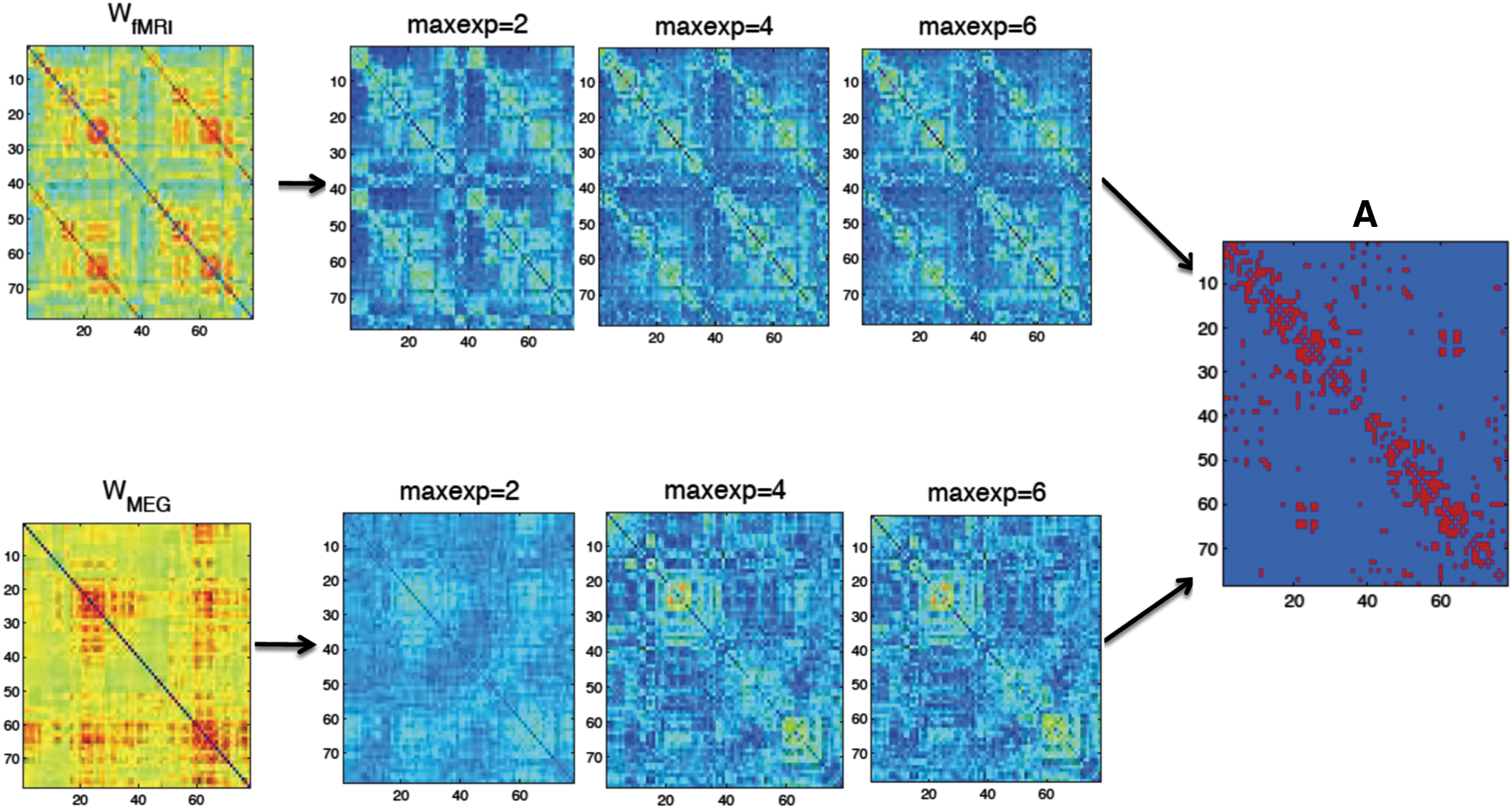
First, we estimated the coefficients in Eq. (5) for the mapping from structural networks to functional networks at the group level (see Supplementary Table S1 for K = 6). For both modalities, we can observe that the SSEnorm becomes lower, that is, the fit becomes better, for increasing number of terms (Fig. 2). Similarly, with an increasing number of fitted coefficients in Eq. (5), the patterns of the fitted functional connectivity matrices resemble better the empirical fMRI and MEG connectivity matrices (Fig. 3, for a complete list of the ROIs see SI-B.1).
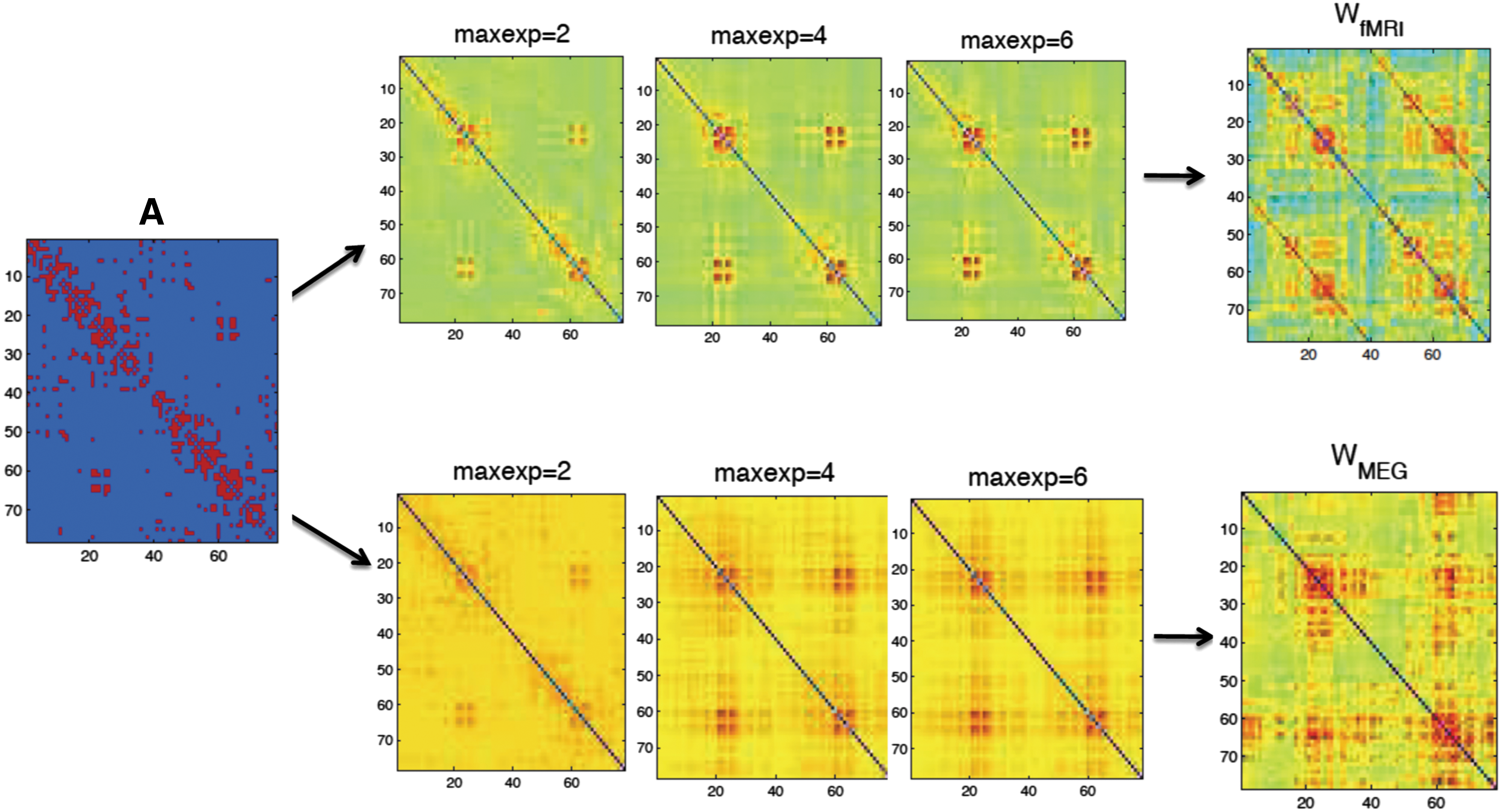
Visualization of the fitted matrices for different maximally fitted exponents K (abbreviation: maxexp) for the function f: A → W
fMRI and f: A → W
MEG versus the empirical matrices for the group-averaged data set. Color images available online at
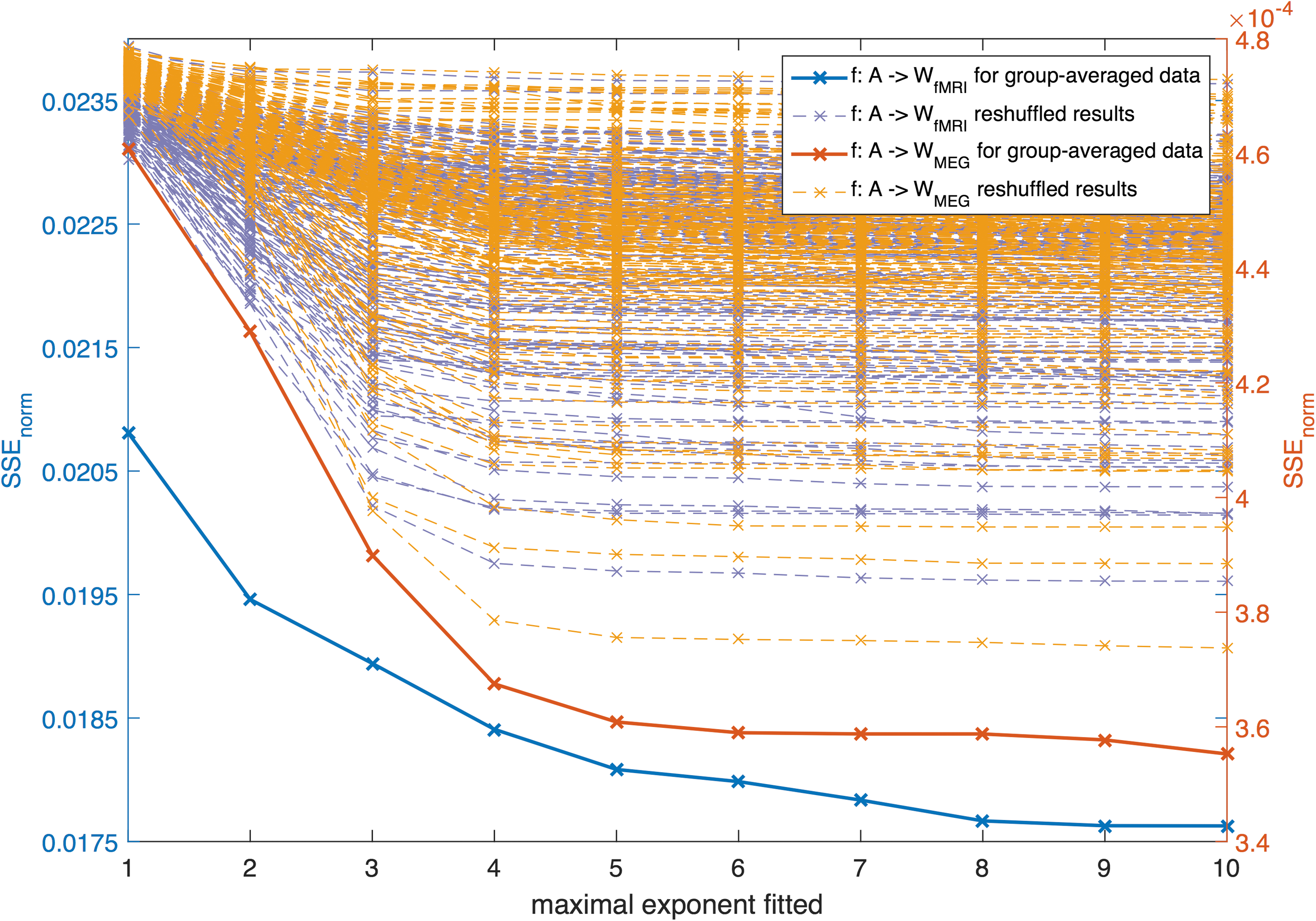
SSEnorm for the group-averaged data set for different maximally fitted exponents K displayed together with the results of the reshuffled matrices. For each mapping, we ran the same analysis with 100 reshuffled versions of the matrix A and with 100 reshuffled versions of matrix W. SSE, sum of squared errors. Color images available online at
However, for the group-averaged data, there seems to be a limit for the number of terms, since including terms of 6th order and higher did not significantly improve the estimation anymore for both MEG and fMRI under the 5% significance level. For these group-averaged networks, the best fit was reached for the mapping f: A → W MEG. We obtained significantly different values of the estimated coefficients for the two different modalities under the 5% significance level (see Supplementary Fig. S10, 95% confidence intervals did not overlap), indicating a modality-dependent mapping.
For the mapping f: A → W fMRI, estimated coefficient values showed a clear decrease when going from lower- to higher-order terms, indicating that lower-order terms in the expansion Eq. (5) contribute more to the estimation of the fMRI network (Supplementary Fig. S10). For the mapping f: A → W MEG, this steep decline in coefficients for higher-order terms was not observed (see Supplementary Fig. S10). The SSEnorm for the data set of individual healthy controls was slightly higher (i.e., worse) than for the group-averaged matrices (Fig. 4). Similar to the group level results, the mapping from structural to MEG networks provided better fits than from structural to fMRI networks also at the individual level.
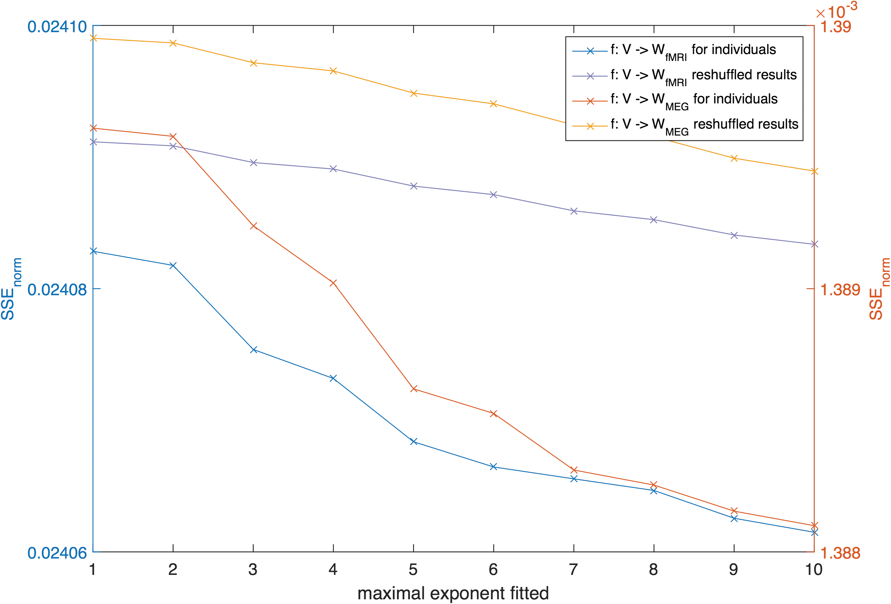
SSEnorm for the individual data set for different maximally fitted exponents K (after averaging over all 11 individual SSEnorm results) displayed together with the averaged result of the reshuffled matrices. For each mapping, we ran the same analysis with 100 reshuffled versions of the matrix V and with 100 reshuffled versions of matrix W. Color images available online at
We repeated the same analysis where either the structural or functional connectivity matrices were substituted by a reshuffled version of the empirical matrix (for details see SI-G). The results of this analysis are also displayed in Figure 2, showing a higher SSEnorm for all reshuffled cases compared to the original matrices, that is, the empirical results differed significantly (p < 0.001) from the reshuffled results. In addition, we observe that the decline in SSEnorm was in most cases for the reshuffled matrices, rather narrow in comparison with the empirical matrices (Fig. 2). Thus, the observed relationship between structure and function can hardly be reproduced by any reshuffled versions of the matrices.
For individual networks, the average performance of the reshuffled matrices was also worse than the empirical original results (Fig. 4). We tested the empirical results versus their reshuffles for significant difference with a Mann–Whitney–Wilcoxon (MWW) test and displayed the p-values in Table 1. From these test results, we can conclude that the mapping f: V → W fMRI was able to outperform its random reshuffle for all subjects (see Table 1). However, the goodness of fit for the mapping f: V → W MEG was for 5 out of 11 subjects, not better than the random reshuffles, indicating that the relation between the two matrices is less unique than for the anatomical matrix and the fMRI matrices.
p-Values for the Comparison Between SSEnor m for the Empirical and Reshuffled Matrices
The matrix V denotes the structural network matrices for the individual data and the different columns are for the different 11 analyzed persons (p1 till p11). Note that in most cases a significantly better goodness-of-fit was obtained for the empirical matrices than for the reshuffled matrices (p < 0.05, indicated with *).
fMRI, functional MRI; MEG, magnetoencephalography; SSE, sum of squared errors.
To cross-validate our mapping, we ran the same analysis on a second group-averaged data set (with similar processing pipeline) and found overlapping confidence intervals for the estimated coefficient values (Figs. 5 and 6).

Estimated coefficients for the mapping f: A → W
MEG for K = 5 together with their 95% confidence interval for the first group-averaged data set and a second group-averaged data set. Color images available online at
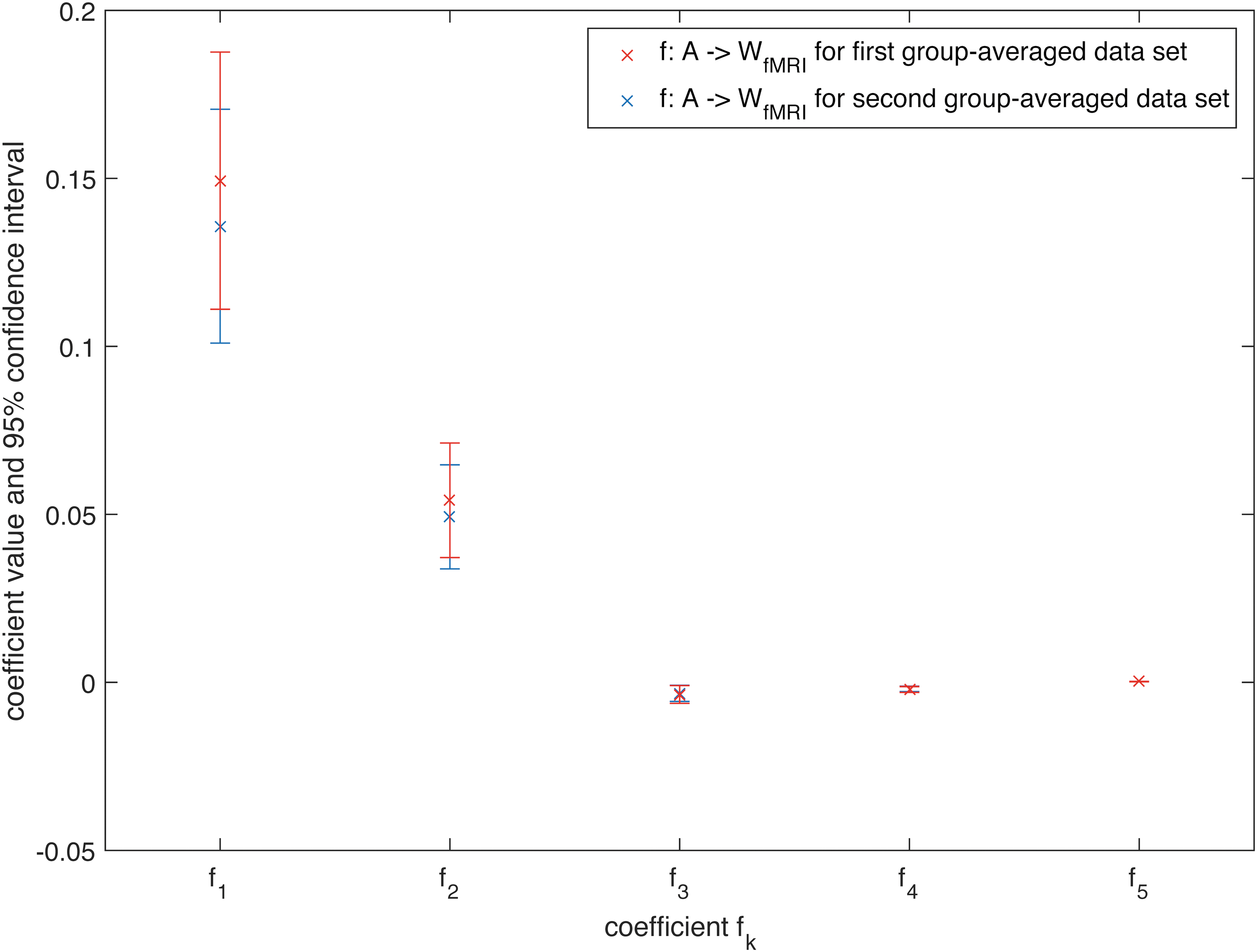
Estimated coefficients for the mapping f: A → W
fMRI for K = 5 together with their 95% confidence interval for the first group-averaged data set and a second group-averaged data set. Color images available online at
Mapping functional networks to structural networks
By reversing the role of A and W and following the same approach as before, we obtained goodness of fit values for the inverse mapping. More specifically, for the group-averaged data, we acquired better fits when starting from W fMRI than from W MEG (see Figs. 7 and 8). Similar to the mapping from structural to functional networks, the estimated coefficients were significantly different under the 5% significance level for the two modalities for the group-averaged data pointing toward a modality-dependent mapping (see Supplementary Fig. S11, 95% confidence intervals did not overlap). An overview of the estimated coefficients for this data set is given in Supplementary Table S1.
Visualization of the fitted matrices for different maximally fitted exponents K (abbreviation: maxexp) for the function f
−1: W
fMRI→A and f
−1: W
MEG→A versus the empirical matrices for the group-averaged data set. Color images available online at
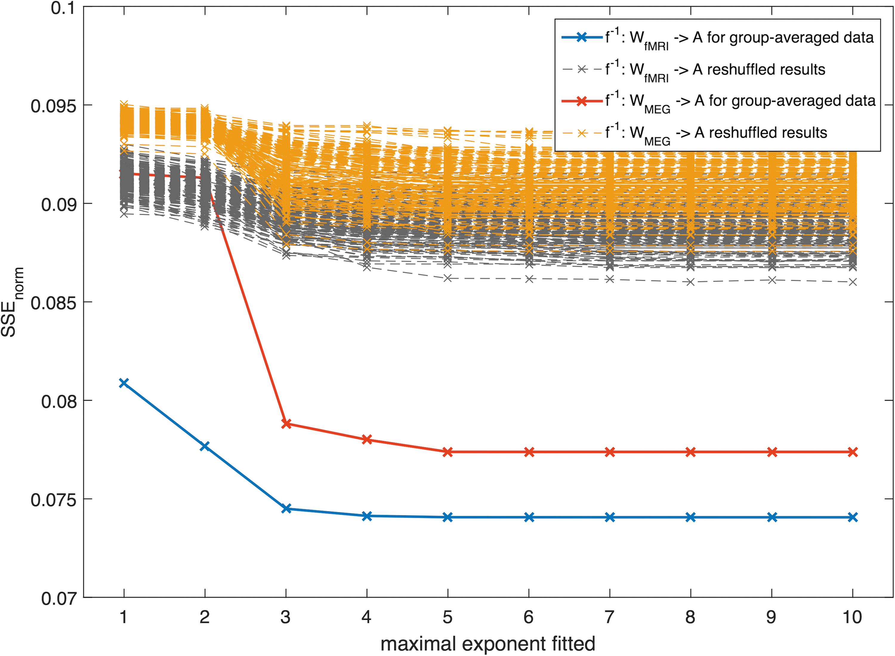
SSEnorm for the group-averaged data set for different maximally fitted exponents K displayed together with the results of the reshuffled matrices. For each mapping, we ran the same analysis with 100 reshuffled versions of the matrix A and with 100 reshuffled versions of matrix W. Color images available online at
Furthermore, similar to the mapping f, no significant improvement of the goodness of fit level was found by including terms of a higher order than 5 for f −1: W MEG→A. Even including W 5 fMRI in the mapping f −1: W fMRI→A hardly improved the fit (no significant improvement under the 5% significance level). Applying the same approach for the individual data, we were able to reach a lower overall error, thus a better fit, for f −1 than for f and the differences in modalities with respect to the residuals were very small for f −1 (see Fig. 9).
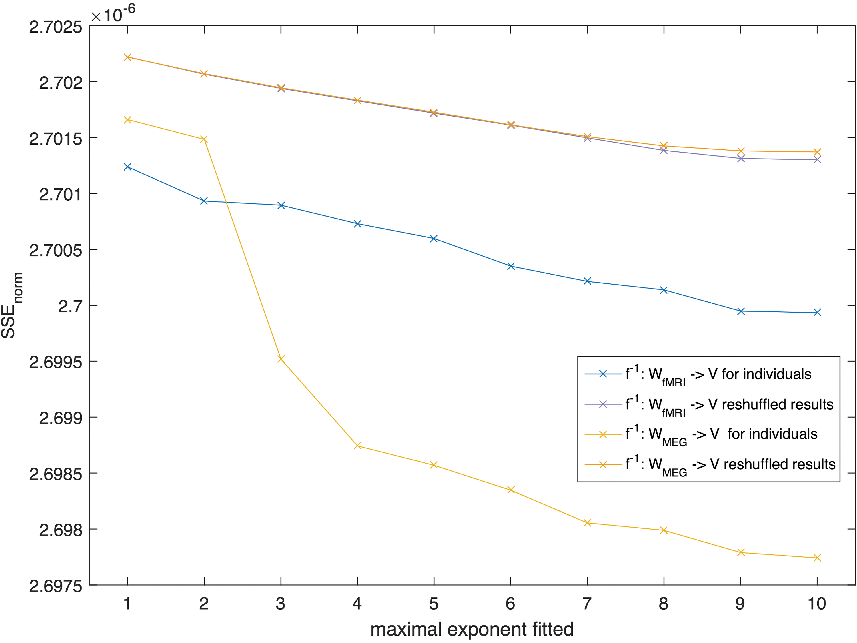
SSEnorm for the individual data set for different maximally fitted exponents K (after averaging over all 11 individual SSEnorm results) displayed together with the averaged result of the reshuffled matrices. For each mapping, we ran the same analysis with 100 reshuffled versions of the matrix V and with 100 reshuffled versions of matrix W. Color images available online at
To have a benchmark for the overall residuals, we again repeated the same analysis with reshuffled matrices. Similar to f, the function f −1 outperformed the random reshuffles for group-averaged networks (see Fig. 7, p-value of 0% for MWW-test). On the subject level, the function f −1 obtained significantly better results for the empirical matrices than their random reshuffles for most of the individuals under the 5% significance level (two outliers for the p-values of the MWW-test for f −1: W fMRI→A, see Table 1 and Fig. 9).
Again, the same analysis using the second group-averaged data set for MEG revealed significant differences only for the estimated coefficients c 1[f] and c 2[f] from Eq. (5) between the first and the second data set (for K = 5, Figs. 10 and 11). For fMRI, a significant difference could only be determined for c 1[f], but not for the other estimated coefficients from Eq. (5), which again cross-validates our mapping between different data sets.
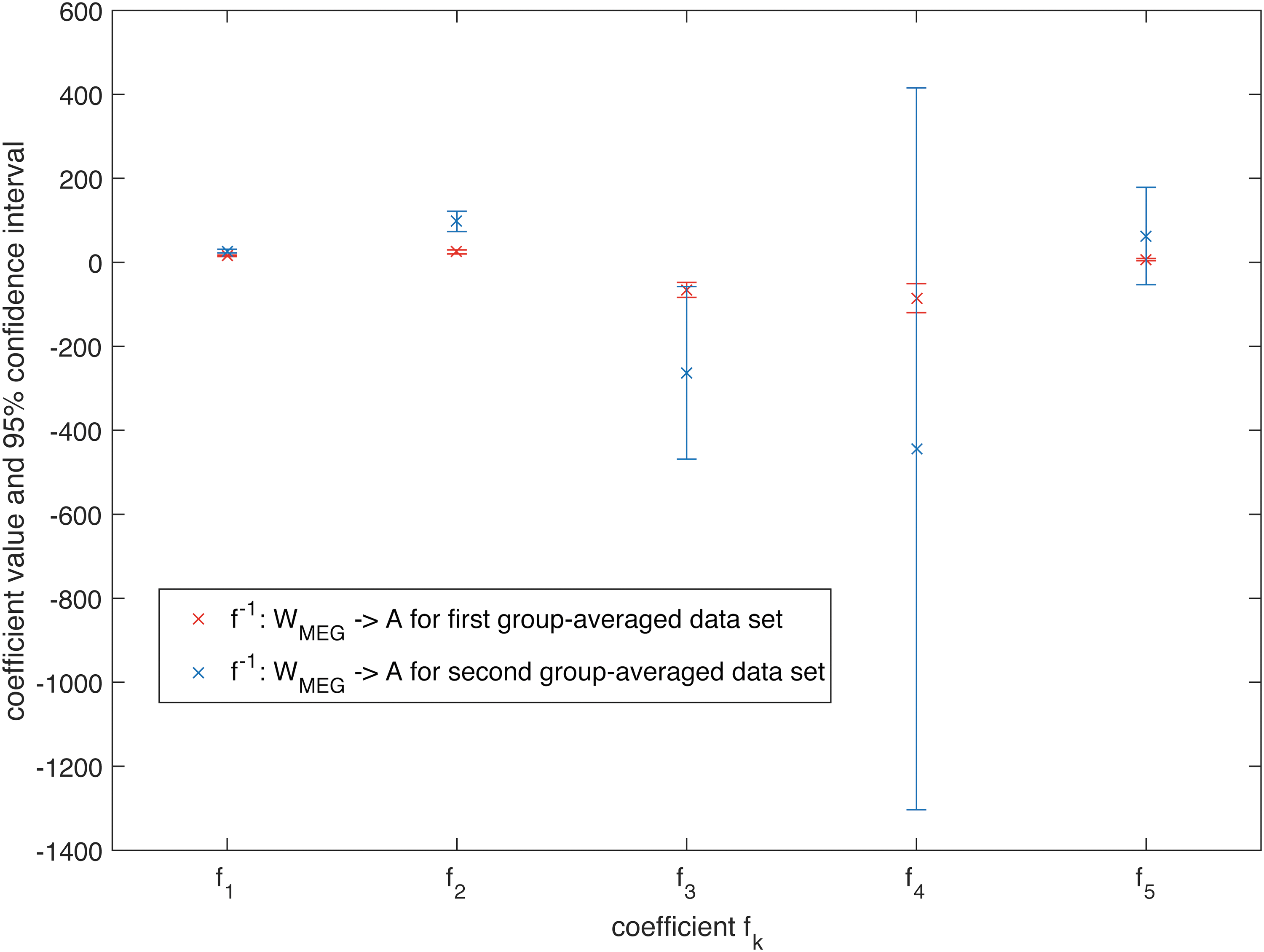
Estimated coefficients for the mapping f
−1: W
MEG→A for K = 5 together with their 95% confidence interval for the first group-averaged data set and a second group-averaged data set. Color images available online at
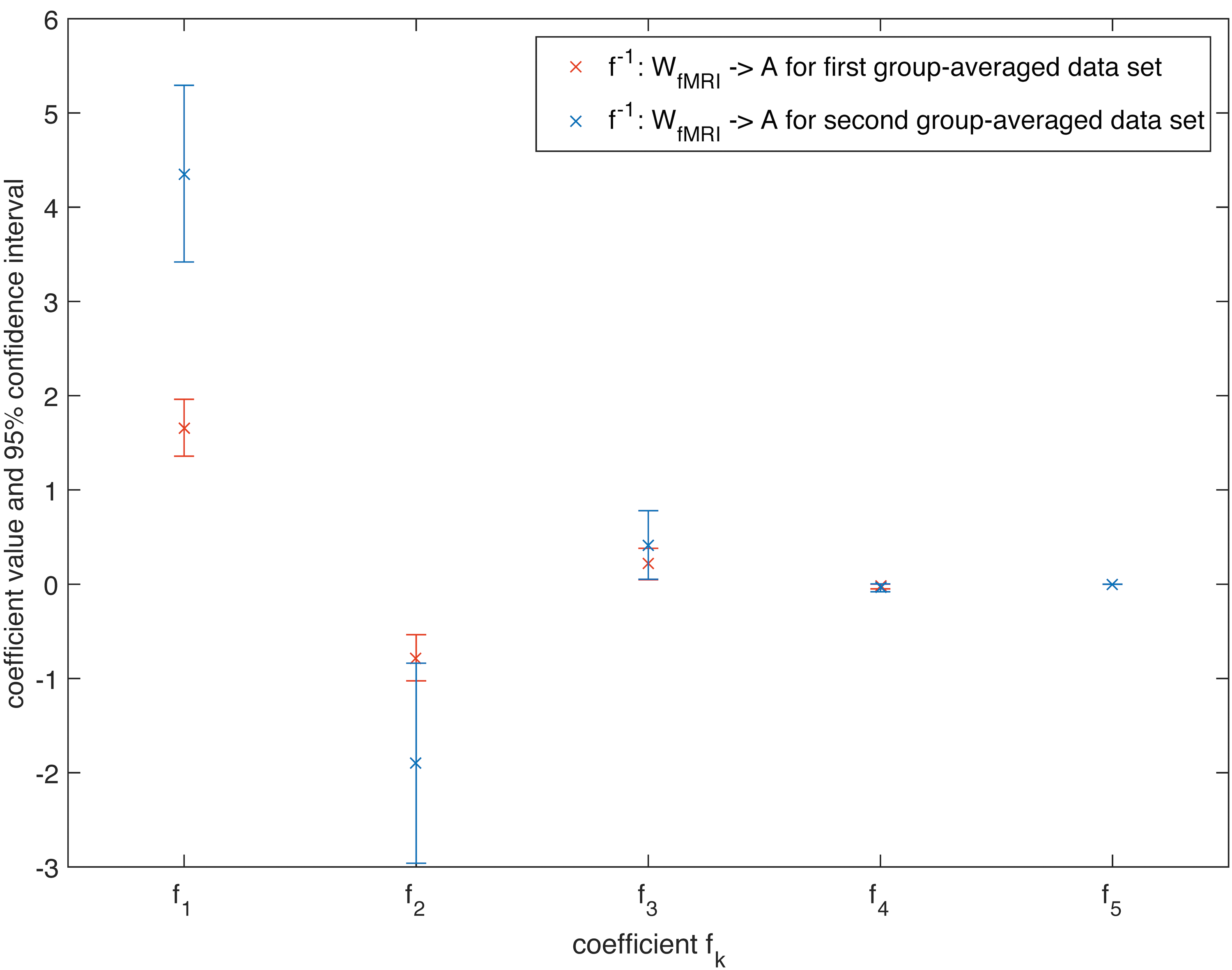
Estimated coefficients for the mapping f
−1: W
fMRI→A for K = 5 together with their 95% confidence interval for the first group-averaged data set and a second group-averaged data set. Color images available online at
Moreover, the whole analysis was repeated multiple times to check for the stability of the estimated coefficients, which resulted in exactly the same coefficients every time, underlining the robustness of our results. We also analyzed in more detail which connections were well predicted by our approach and which were estimated less accurately (see Supplementary Figs. S16–S23). A corresponding analysis in the spectral domain (see SI-B.2 for the results) illustrated that the estimated coefficient values were similar to those in the topology domain for the function f, but not for f −1 (see Supplementary Figs. S6–S9). The dissimilarities between the spectral and topology domain are most probably due to eigenvector perturbations between the different analyzed empirical matrices. These eigenvector perturbations can probably be traced back to noisy measurements (see SI-F).
Discussion
In this study, we have analyzed the mutual dependency of structural and (resting-state) functional networks in a multimodal framework by assuming that there exists a mathematical function that allows for a mapping between the two networks. This function was then analyzed without assuming a priori any specifics and by estimating the coefficients for the mappings in both directions (i.e., structural to functional and functional to structural networks). Our analysis convincingly implicated that our assumption of a mapping between the two networks was justified because we reached overall good fits outperforming random reshuffles and resulting in similar matrix patterns. However, our results also indicated that the mapping was modality dependent as the coefficients for mappings with MEG- or fMRI-based networks significantly differed.
The existence of such a mathematical function points toward the fact that the functional connectivity of the brain can be described by a combination of the underlying structural connections. Because of the stability of the estimated coefficients and their cross-validation across different data sets, such a mathematical function could potentially be used to predict structure from function or vice versa in future studies. Also, once we can use this mathematical framework to predict “healthy” functional connectivity, we can compare the matrix to the actual measured functional network of the patient and identify possible malicious connections indicating disease.
Neurobiological interpretation
If we consider the case of a binary structural adjacency matrix, then the matrix element (A k)ij equals the number of walks of length k between node i and node j. Each term c k[f]A k can be considered the contribution of walks with hopcount k to the functional network (see Supplementary Fig. S12). In this study, hopcount is defined as the number of intermediate links between two nodes in a walk (length of the walk). Our approach confirms the ideas postulated by Robinson and coworkers that a functional connection can be regarded as a sum of all possible walks between two regions (Robinson, 2012; Robinson et al., 2014). In addition, our approach returns the coefficients c k[f], which can be interpreted as the influence of all walks with hopcount k (see Supplementary Table S1 and Supplementary Fig. S12).
In contrast to a path, a walk can traverse the same node more than once. Potential loops in walks are also in line with the belief that reentry loops can act as a resonating system to enhance a signal that needs to be spread over a long distance (Goñi et al., 2014).
In contrast to most previous studies, we followed a multimodal approach analyzing the mapping for MEG and fMRI data. As opposed to studies that assumed a specific function beforehand, we followed a data-driven approach by fitting coefficients of the general expression Eq. (5). More precisely, fMRI networks seemed to be shaped by walks of lower hopcount in the structural network since the coefficients were higher for these configurations (see Supplementary Fig. S10). In contrast, for MEG networks all walks from the underlying structural network up to hopcount 5 appeared to contribute more or less equally to the resulting fitted functional network matrix (see Supplementary Fig. S11). Overall, we found that estimations from structural networks were more accurate when predicting MEG networks on both individual and group level than when predicting fMRI networks.
However, when the functional network was used to predict the structural one, we saw only small differences at the individual level between the modalities, but at the group level the fitting using fMRI matrices performed better. These observations together with the significantly different coefficients for MEG and fMRI confirm the modality dependency of the mapping.
If ρ denotes the diameter of the network, defined as the hopcount of the longest shortest path in a graph (Van Mieghem, 2011), our analysis for both fMRI and MEG suggests that the diameter of the unweighted structural network (ρ = 6) is directly related to the number of terms K = 5 in Eq. (5) that are sufficient for the best fit of the mapping from structural to functional networks. Hence, a functional connection between two regions seems only to be shaped by walks in the structural network that are shorter than the diameter of this structural network. The important role of the diameter in this fitting procedure can also be mathematically justified (see also SI-A.2).
Besides the possibility of predicting the functional network using the structural network, our analysis also has practical implications on how communication processes the shape brain activity. Bullmore and Sporns (2012) proposed the hypothesis that the brain is optimized for efficiency and robustness. Our findings seem to be in line with this idea since the brain seems to use not only (structural) shortest paths (most efficient from a network perspective) for communication but is also transmitting information through less-efficient paths or walks. Thus, there seems to be some kind of degeneracy in the brain (Price and Friston, 2002). From a network science perspective, spreading information not only through the shortest path makes the (healthy) brain function more robust against link breakage.
However, there seems to be an upper bound for the length of the paths that the brain uses for communication, which corresponds to the diameter of the structural brain network. Walks that are longer than the diameter are highly inefficient for communication. The diameter therefore seems to symbolize the trade-off between efficiency and robustness (Bullmore and Sporns, 2012). It is this degeneracy and robustness that could keep two regions functionally connected when the direct structural connection is damaged in disease.
In multiple sclerosis, the structural network gets damaged due to lesions and diffused white matter damage. With this theory we could predict which detours are likely to be taken for functional connections to uphold (sub)-optimal network efficiency. Thus, based on the damaged structural network, we could be able to make predictions on how this damaged structural network might map on a functional network. These practical implications seem to agree with several studies that have shown that the averaged path length is higher in diseases than in the healthy brain (Stam, 2014).
Our mathematical approach incorporates previous models on the relationship between structural and functional networks into one single model. For example, a previous study found that the shortest paths and detours along these paths in the structural network were the strongest predictors for functional connections (Goñi et al., 2014). This result agrees with our finding of the structural–functional network mapping being dependent on the combination of walks with small hopcounts (corresponding to the shortest paths in the network) and detours from these shortest paths. Also, the suggestion that network diffusion has the ability to predict functional connections (Abdelnour et al., 2014) is in line with our work. Network diffusion indicates that information is not merely transmitted through the shortest paths, but also through less-efficient paths.
Furthermore, our mathematical function also includes the predictive value of common neighbors for functional connections (Vértes et al., 2012). The term c 2 [f]A 2 in Eq. (5) corresponds to the weighted number of walks between any pair of nodes with hopcount 2, that is, walks from any node i to a node j through a common neighbor. In a previous study, Tewarie and coworkers (2014) demonstrated that the degree product between nodes in the structural network together with the Euclidean distance has the ability to predict the functional connections between these nodes. We observed in this study that our approach with the sum of structural matrices A k in Eq. (5) is correlated not only with the degree product (Supplementary Fig. S13) but also with the complete previous model (including Euclidean distance, Supplementary Fig. S14).
Predicting the structural network from the functional network has received relatively little attention (Abdelnour et al., 2014; Deco et al., 2014; Robinson, 2012; Robinson et al., 2014). We assumed that the structural network is a weighted sum of powers of the functional network matrix W. However, unlike the structure-to-function mapping f, the interpretation of this mathematical function is less straightforward: If we define the weight of a walk as the product of all weights along this walk, then the matrix entry (W k)ij represents the summed weights of all possible walks with hopcount k between node i and node j. Similar to the function f, we find for f −1 that higher powers of W do not contribute substantially to the goodness of fit of our mapping.
In contrast to the powers of a binary matrix, W k does not only contain the number of walks with hopcount k but also incorporates information about their weight structure. Still, we can conclude that longer walks in the functional network seem to influence the structural brain network less. Practically, this result not only helps us to reconstruct the structural connections when we have only the functional connectivity matrices but also indicates that a direct structural connection between two brain regions seems to be influenced not only by their direct functional connectivity but also by the (functional) communication within a small hopcount neighborhood of those two regions.
Using an additional data set of individual healthy controls [data set (iii)], we found that our mapping can also be generalized to the individual level. For the individual mappings, we also found that nearly all mappings were able to outperform their reshuffled benchmark except for some outliers (see Table 1). Furthermore, we compared the results of the group-averaged data and the individual data (each of these containing data from multiple modalities). In the case of the mapping from structural to functional networks, the performance when using individual fits was similar to that obtained when using the group-averaged matrices (see Figs. 2 and 4).
However, for the inverse mapping, the individual mappings provided a much better fit than the group-averaged mappings. These results could potentially be explained by the following factors: (1) there exists an even stronger relationship between function and structure at the individual level, (2) the use of weighted structural connectivity matrices (instead of the binary group-averaged structural connectivity matrix), which are more representative of the underlying fiber bundle structure, or (3) the fact that the structural and functional information were gathered from the same group for data set (ii) (in contrast, the group-averaged structural and functional connectivity matrices were based on two different sets of healthy controls).
Technical implications
Our approach may provide important information about the DTI-obtained structural network that is generally missed due to methodological issues with crossing versus kissing fibers, which usually affect interhemispheric connections. Given the functional networks, a mapping to the structural network could also allow to distinguish between genuine and false positive connections, which are inherently present in DTI data (Thomas et al., 2014). For example, in the structural networks estimated from MEG and fMRI networks, we observed more homologous interhemispheric connections than in the actual empirical structural network (see the off-diagonal in Supplementary Fig. S3).
In addition, for MEG functional connectivity metrics, there are well known methodological issues with volume conduction, signal leakage, and field spread. By using our approach and trying out different functional connectivity metrics, one could aim to find the common properties of these mappings, that is, those that are invariant of the functional metric that was used.
Methodological considerations
First, we investigated the relationship between the structural network and static patterns of (resting-state) functional connectivity, as functional connectivity was estimated over epochs of several seconds. Therefore, our approach does not consider the dynamical aspects of functional connectivity. It is well known that functional networks obtained from smaller time windows correspond less to the structural network (Honey et al., 2007; Messé et al., 2014; Ton et al., 2014) and therefore our approach could be less applicable to these smaller time scales.
Second, the mapping employed in this study can certainly be influenced by the choice of the parcellation of brain regions. However, as long as the ratio between genuine (functional or structural) connections and noise in the matrices remains similar between parcellation atlases, we do not expect it to have a significant impact on the goodness of fit of our mapping. Despite the well-known limitations of the AAL atlas, it still provides a commonly used framework in neuroimaging studies. By using it, the results from our study are directly relevant for this existing body of work. We also provided a suggestion of how to overcome the dimension differences of the matrices of different parcellations mathematically in SI-I.
Third, our mapping can be influenced by noise in the matrices, such as the presence of false positives in the structural connectivity matrix. However, by randomly adding some connections on top of the existing connections to the structural network and redoing the analysis, we observed that the fluctuation in goodness of fit was relatively small (see Supplementary Fig. S15).
Fourth, we have chosen the alpha2 band because of high SNR for this frequency band. The mapping between structure and function may be different in terms of coefficients for the other frequency bands because we face there is to some extent a different structure in the matrices. To explore the mapping for different frequency bands is a goal for future studies. Since the PLI probably underestimates the connectivity strengths (Stam et al., 2007), future research should apply our methods on other connectivity measures as well, which will probably lead to different mappings in terms of different coefficients. Previous studies have used the amplitude envelope correlation to study MEG/fMRI similarity (Brookes et al., 2011). This metric may be used in future studies to analyze structural versus functional network mappings, but this is beyond the scope of this study.
Conclusion
In this study, we have demonstrated that, irrespective of the functional imaging modality, the relationship between structural and functional networks can be described by a mapping. Such a mathematical function can predict resting-state functional networks from the structural network and vice versa. This mathematical function can be described by a weighted sum of matrix powers, which represent, in the binary case, the number of walks up to a certain hopcount in the network. Thus, according to our analysis, a functional connection seems to be shaped by shorter walks up to the diameter in the underlying structural network.
This result provides a general framework that incorporates previously published models on the relationship between structural and (stationary) functional networks. Also, when analyzing the mapping from functional to structural networks, longer walks in the functional brain network appear not to have a big influence on the structural connections. We found different coefficients for MEG and fMRI for our mapping, which point toward a modality dependency for the structure–function relationship.
Furthermore, this mathematical function could help to reduce noise and artifacts for the empirical estimation of structural and functional networks. We were also able to extend this mapping relationship to the subject level. For future work, differences in individual mappings between patients and healthy controls may provide insights in the disrupted relationship between the structural and functional brain networks in various diseases.
Footnotes
Acknowledgments
This work was partially supported by a private sponsorship to the VUmc MS center Amsterdam. The VUmc MS center Amsterdam is sponsored through a program grant by the Dutch MS Research Foundation (grant number 09-358d). We thank Menno Schoonheim for acquisition and postprocessing of fMRI data. We also thank Gaolang Gong for providing structural network data. We thank Cornelis J. Stam for his useful comments and input that improved the article.
Author Disclosure Statement
No competing financial interests exist.
References
Supplementary Material
Please find the following supplemental material available below.
For Open Access articles published under a Creative Commons License, all supplemental material carries the same license as the article it is associated with.
For non-Open Access articles published, all supplemental material carries a non-exclusive license, and permission requests for re-use of supplemental material or any part of supplemental material shall be sent directly to the copyright owner as specified in the copyright notice associated with the article.