Bridging the Gap: Dynamic Causal Modeling and Granger Causality Analysis of Resting State Functional Magnetic Resonance Imaging

Abstract

Granger causality (GC) and dynamic causal modeling (DCM) are the two key approaches used to determine the directed interactions among brain areas. Recent discussions have provided a constructive account of the merits and demerits. GC, on one side, considers dependencies among measured responses, whereas DCM, on the other, models how neuronal activity in one brain area causes dynamics in another. In this study, our objective was to establish construct validity between GC and DCM in the context of resting state functional magnetic resonance imaging (fMRI). We first established the face validity of both approaches using simulated fMRI time series, with endogenous fluctuations in two nodes. Crucially, we tested both unidirectional and bidirectional connections between the two nodes to ensure that both approaches give veridical and consistent results, in terms of model comparison. We then applied both techniques to empirical data and examined their consistency in terms of the (quantitative) in-degree of key nodes of the default mode. Our simulation results suggested a (qualitative) consistency between GC and DCM. Furthermore, by applying nonparametric GC and stochastic DCM to resting-state fMRI data, we confirmed that both GC and DCM infer similar (quantitative) directionality between the posterior cingulate cortex (PCC), the medial prefrontal cortex, the left middle temporal cortex, and the left angular gyrus. These findings suggest that GC and DCM can be used to estimate directed functional and effective connectivity from fMRI measurements in a consistent manner.

Introduction

Over the past years, many techniques have been proposed to characterize how brain areas interact with each other, under different experimental conditions. Several neuroimaging studies are available, describing neuronal dynamics under rest and task, considering the merits and demerits of different approaches. The concepts of directed functional connectivity and effective connectivity have become prominent in neuroimaging research (Friston, 1994). Directed functional connectivity, for example, Granger causality (GC) (Granger, 1969), assesses the recurrent functional integration, among different brain areas. This approach is exploratory and rests on the notion of predictability and statistical dependencies to establish causal relationships. On the contrary, effective connectivity—as measured with dynamic causal modeling (DCM) (Friston et al., 2003), considers the influence of one neural system over the other. DCM is based on theoretical assumptions and specifies different hypotheses in terms of different models or architectures.

GC and DCM are the predominant techniques for exploring directed coupling or connectivity among brain regions using electroencephalography (EEG), magnetoencephalography (MEG), and functional magnetic resonance imaging (fMRI) data. However, both have been a topic of debate for some time. GC has been used to provide useful descriptions of directed functional connectivity using electrophysiological data (Bastos et al., 2015; Bernasconi et al., 1999; Brovelli et al., 2004; Ding et al., 2000), electrocorticographic data (Bosman et al., 2012), MEG or EEG data either at the source or sensor level (following spatial filtering) (Barrett et al., 2012), and spike train data derived from single-unit recordings (Kim et al., 2011). Applications of GC to fMRI time series have been considered as contentious because GC does model the hemodynamic generation of observed signals from underlying neuronal states (Friston, 2011b, 2009; Roebroeck et al., 2011). FMRI studies suggest that the hemodynamic response function (HRF) varies over the brain regions and individuals (Aguirre et al., 1998), which can confound the temporal precedence of neuronal events assumed by GC. However, GC is a well-accepted measure in the analysis of electrophysiological time series, because of zero temporal lag between observed responses and their neuronal causes (Brovelli et al., 2004; Friston et al., 2013). Seth et al. (2013) showed both theoretically and in a series of simulations that Granger causal inferences are robust to a wide variety of changes in hemodynamic response properties, noting that severe downsampling and/or excessive measurement noise in fMRI data may lead to incorrect inferences.

In contrast to GC, DCM relies on probabilistic graphical models of distributed dynamics, which are specified in terms of priors on connectivity or coupling parameters. It assumes that causal interactions among brain areas are mediated by hidden neuronal dynamics, specified in terms of nonlinear differential equations in continuous time. The parameters of these equations reflect the connection strength, which are estimated using Bayesian techniques (Stephan et al., 2010). DCM eludes the controversies related to variations in the HRF because it models (regionally specific) hemodynamic and neuronal state variables that generate observed data. Furthermore, it has been shown that DCMs, which include hidden regions, outperform equivalent DCMs, based only on regions that can be observed directly. For example, Boly et al. (2012) showed that a DCM that included a hidden thalamic source outperformed an equivalent DCM based only on cortical sources. Hence, GC and DCM are based on different assumptions and ideas, but both model neural interactions and are concerned with directed causal interactions—and both may provide complementary or even consistent perspectives (Friston et al., 2013; Valdes-Sosa et al., 2011).

In the current study, we used the GC and DCM techniques to analyze resting state fMRI (rsfMRI) data and compared the resulting connectivity estimates. We assumed that both GC and DCM could be applied to a common data set to ask whether the connectivity parameters obtained from both techniques show similar connectivity or network architecture.

We applied GC and DCM to simulated fMRI time series data and to empirical rsfMRI data. For the simulations, we used a stochastic integration scheme, with random fluctuations on neuronal activity driving hemodynamic states—under a simple (linear) model of neuronal coupling—to generate simulated fMRI time series data for two nodes. For posterior estimates, we used a Bayesian filtering approach in generalized coordinates over the simulated data (Friston et al., 2010). The nonparametric GC (Dhamala et al., 2008a) approach was then applied to the same simulated data to examine the direction of the information flow between these nodes and to compare the results with those of DCM.

For the empirical data, we selected four brain regions of default mode network (DMN): the posterior cingulate cortex (PCC), the medial prefrontal cortex (mPFC), the left middle temporal cortex (LMTC), and the left angular gyrus (LAG), all of which are anatomically connected (Bajaj et al., 2013). We performed connectivity analysis; applying GC and DCM on the resulting rsfMRI data, collected from 17 healthy subjects. Nonparametric GC (Dhamala et al., 2008a) was applied to characterize the network interactions among these four nodes, and net in-degree was calculated for each node. We then applied DCM to the same data by defining a model space that allowed for various combinations of connections. Finally, we compared the optimal model and its connectivity parameters—obtained from Bayesian model selection (BMS) and Bayesian model averaging (BMA), respectively—with the corresponding estimates of GC.

Materials and Methods

Participants

We collected resting state fMRI data from 17 participants (mean age: 25.2 ± 4.7 years, 12 males, 5 females). All the participants had normal neurological functioning and normal or corrected to normal visual acuity. A written consent was obtained from each participant before the experiment, and all the participants were compensated for their participation and time. Georgia State University Institutional Review Board and the Joint Institutional Review Board of Georgia State University and Georgia Institute of Technology, Atlanta, approved experimental protocol. All the participants were instructed to be at rest and relax with their eyes open, focusing at the central cross on a computer screen.

Imaging

All the functional data were collected at BITC (Georgia Tech and Emory University Biomedical Imaging Technology Center, Atlanta) using 3-Tesla Siemens whole-body MRI scanners. Functional imaging was 7 min and 54 sec long and included a T2*-weighted echo planner imaging (EPI) sequence (echo time [TE] = 40 ms; repetition time [TR] = 2000 ms; flip angle = 90°; field of view [FOV] = 24 cm, matrix = 64 × 64; number of slices = 33 and slice thickness = 5 mm). High-resolution anatomical T1-weighted images were acquired for anatomical references using a magnetization-prepared rapid gradient-echo (MPRAGE) sequence with an isotropic voxel size of 2 mm.

Conventional image analysis

FMRI data were preprocessed using SPM8 (Wellcome Trust Centre for Neuroimaging, London; www.fil.ion.ucl.ac.uk/spm/software/spm8/), with slice time correction, motion correction, coregistration, normalization, and spatial smoothing. Motion correction to the first functional scan was performed within participant, using a six-parameter rigid-body transformation. The mean of the motion-corrected images was coregistered to the individual structural image using a 12-parameter affine transformation. The images were then spatially normalized to the Montreal Neurological Institute (MNI) template (Talairach and Tournoux, 1988) by applying a 12-parameter affine transformation, followed by a nonlinear warping using basis functions (Ashburner et al., 1999). Furthermore, images were smoothed with an 8-mm isotropic Gaussian kernel and high pass filtered in the temporal domain (to remove low-frequency drifts).

Regions of interest

For functional connectivity maps, we used the seed-based correlation approach, choosing the PCC as a seed region (Fox et al., 2009) with an 8 mm radius sphere centered at −6, −52, 40 in MNI coordinate system (Chang and Glover, 2010; Fox et al., 2009). MARSBAR software package (http://marsbar.sourceforge.net/) was used to create masks and extract blood oxygen level-dependent (BOLD) time series for further network analysis. Time series from a further three regions, namely, mPFC (0, 48, −4), LMTC (−57, −19, −11), and LAG (−46, −64, 25), were significantly positively correlated to PCC (p < 0.05). Coordinates of these regions are reported in MNI coordinate system. All these regions are known to be anatomically connected to each other (Bajaj et al., 2013).

For effective connectivity analysis using DCM, the above regions of interest (ROIs) were defined in SPM12 (www.fil.ion.ucl.ac.uk/spm/software/spm12/) using the first eigen variate of activations within a sphere of radius 8 mm in the MNI coordinate system. Central coordinates for all the ROIs were same for both analyses.

Dynamic causal modeling

DCM is based on dynamical systems theory: activity in one area causes dynamics in another and this dynamics causes observations. The aim of DCM is to estimate the directed connectivity mediating the dynamics or interactions among functionally connected brain areas (Friston et al., 2003; Stephan et al., 2010). Using bilinear approximations to coupled brain states and modeling the influence of external inputs, DCM detects the coupling between brain regions. Different models are constructed, where each model has specific intrinsic connections that are modulated by different external changes. Bayesian model selection is based on the exceedance probability. This is a measure used to compare the posterior probabilities of alternative models to find the “winning” model (Stephan et al., 2009). BMS explores the model space, scoring each model in terms of its model evidence. To infer model parameters, one generally uses BMA (Penny et al., 2010; Stephan et al., 2010). BMA computes a weighted average of each parameter under each model, where the weighting depends upon model evidence. It is particularly useful when (1) one is interested in determining the strength of a particular connection to compare across groups or (2) there is no clearly winning model or (3) when different subjects have different winning models. In these situations, the Bayesian model average properly accommodates uncertainty about the underlying model; here, connectivity architecture of directed connections.

Granger causality

GC is based on the idea that causes precede and predict their effects. GC can be implemented through parametric (autoregressive [AR] modeling) or nonparametric (spectral factorization based) methods (Dhamala, 2015; Dhamala et al., 2008a). If the AR prediction of the first time series “X1” at present could be improved by including the past information of the second time series “X2”, over and above the information already in the past of X1 itself, one concludes that X2 has a causal influence on X1. The role of X1 and X2 can be reversed to address the causal influence in the opposite direction. The spectral decomposition of Granger's time domain causality was proposed by Geweke (1982, 1984). This characterization identifies the frequency bands over which different areas interact with each other. GC is based on a mathematical framework that extends the well-accepted coherence measure. It rests upon dependencies among data themselves without any reference to how these dependencies are caused. In the current study, we used nonparametric GC approach for pairwise GC calculation (Dhamala et al., 2008a). AR modeling, the basis of the parametric GC technique, has proven effective for the data modeled by low-order AR processes. However, AR methods sometimes fail to capture complex spectral features in the data that require higher order AR models (Mitra and Pesaran, 1999). Nonparametric GC approach bypasses the step of parametric data modeling and combines the spectral density matrix factorization with Geweke's time series decomposition. Using the nonparametric spectral estimation technique on time series for two nodes l and m, spectral density matrix \documentclass{aastex}\usepackage{amsbsy}\usepackage{amsfonts}\usepackage{amssymb}\usepackage{bm}\usepackage{mathrsfs}\usepackage{pifont}\usepackage{stmaryrd}\usepackage{textcomp}\usepackage{portland, xspace}\usepackage{amsmath, amsxtra}\pagestyle{empty}\DeclareMathSizes{10}{9}{7}{6}\begin{document}$$\left[ {S ( f ) } \right]$$ \end{document} , transfer function \documentclass{aastex}\usepackage{amsbsy}\usepackage{amsfonts}\usepackage{amssymb}\usepackage{bm}\usepackage{mathrsfs}\usepackage{pifont}\usepackage{stmaryrd}\usepackage{textcomp}\usepackage{portland, xspace}\usepackage{amsmath, amsxtra}\pagestyle{empty}\DeclareMathSizes{10}{9}{7}{6}\begin{document}$$\left[ {H ( f ) } \right]$$ \end{document} , and noise covariance matrix \documentclass{aastex}\usepackage{amsbsy}\usepackage{amsfonts}\usepackage{amssymb}\usepackage{bm}\usepackage{mathrsfs}\usepackage{pifont}\usepackage{stmaryrd}\usepackage{textcomp}\usepackage{portland, xspace}\usepackage{amsmath, amsxtra}\pagestyle{empty}\DeclareMathSizes{10}{9}{7}{6}\begin{document}$$( \Sigma )$$ \end{document} are obtained (Dhamala et al., 2008a; Ding et al., 2006).

In the frequency domain, using \documentclass{aastex}\usepackage{amsbsy}\usepackage{amsfonts}\usepackage{amssymb}\usepackage{bm}\usepackage{mathrsfs}\usepackage{pifont}\usepackage{stmaryrd}\usepackage{textcomp}\usepackage{portland, xspace}\usepackage{amsmath, amsxtra}\pagestyle{empty}\DeclareMathSizes{10}{9}{7}{6}\begin{document}$$S ( f ) = H ( f ) \Sigma {H^*} (f)$$ \end{document} , where the transfer function \documentclass{aastex}\usepackage{amsbsy}\usepackage{amsfonts}\usepackage{amssymb}\usepackage{bm}\usepackage{mathrsfs}\usepackage{pifont}\usepackage{stmaryrd}\usepackage{textcomp}\usepackage{portland, xspace}\usepackage{amsmath, amsxtra}\pagestyle{empty}\DeclareMathSizes{10}{9}{7}{6}\begin{document}$$H (f )$$ \end{document} and the noise covariance matrix \documentclass{aastex}\usepackage{amsbsy}\usepackage{amsfonts}\usepackage{amssymb}\usepackage{bm}\usepackage{mathrsfs}\usepackage{pifont}\usepackage{stmaryrd}\usepackage{textcomp}\usepackage{portland, xspace}\usepackage{amsmath, amsxtra}\pagestyle{empty}\DeclareMathSizes{10}{9}{7}{6}\begin{document}$$\Sigma$$ \end{document} are derived from spectral matrix factorization, the causality from m to l at frequency f can be calculated as follows: \documentclass{aastex}\usepackage{amsbsy}\usepackage{amsfonts}\usepackage{amssymb}\usepackage{bm}\usepackage{mathrsfs}\usepackage{pifont}\usepackage{stmaryrd}\usepackage{textcomp}\usepackage{portland, xspace}\usepackage{amsmath, amsxtra}\pagestyle{empty}\DeclareMathSizes{10}{9}{7}{6}\begin{document} \begin{align*}{ I_ { m \to l } } ( f ) = \ln { \frac { { S_ { ll } } ( f ) } { { S_ { ll } } (\, f ) - ( { \Sigma _ { mm } } - \Sigma _ { lm } ^2 / { \Sigma _ { ll } } ) \vert { H_ { lm } } (\, f ) { \vert ^2 } } } \tag { 1 } \end{align*} \end{document}

GC values are integrated over the frequency range 0.0021 Hz \documentclass{aastex}\usepackage{amsbsy}\usepackage{amsfonts}\usepackage{amssymb}\usepackage{bm}\usepackage{mathrsfs}\usepackage{pifont}\usepackage{stmaryrd}\usepackage{textcomp}\usepackage{portland, xspace}\usepackage{amsmath, amsxtra}\pagestyle{empty}\DeclareMathSizes{10}{9}{7}{6}\begin{document}$$( {f_1} )$$ \end{document} to 0.1 Hz \documentclass{aastex}\usepackage{amsbsy}\usepackage{amsfonts}\usepackage{amssymb}\usepackage{bm}\usepackage{mathrsfs}\usepackage{pifont}\usepackage{stmaryrd}\usepackage{textcomp}\usepackage{portland, xspace}\usepackage{amsmath, amsxtra}\pagestyle{empty}\DeclareMathSizes{10}{9}{7}{6}\begin{document}$$( {f_2} )$$ \end{document} (Bajaj et al., 2015, 2014): \documentclass{aastex}\usepackage{amsbsy}\usepackage{amsfonts}\usepackage{amssymb}\usepackage{bm}\usepackage{mathrsfs}\usepackage{pifont}\usepackage{stmaryrd}\usepackage{textcomp}\usepackage{portland, xspace}\usepackage{amsmath, amsxtra}\pagestyle{empty}\DeclareMathSizes{10}{9}{7}{6}\begin{document} \begin{align*} iG { C_ { m \to l } } = \frac { 1 } { { { f_2 } - { f_1 } } } \int \limits_ { { f_1 } } ^ { { f_2 } } { { I_ { m \to l } } } (\, f ) df \tag { 2 } \end{align*} \end{document}

Finally, we estimated the total causal flow into a node (total in-degree) m, as follows: \documentclass{aastex}\usepackage{amsbsy}\usepackage{amsfonts}\usepackage{amssymb}\usepackage{bm}\usepackage{mathrsfs}\usepackage{pifont}\usepackage{stmaryrd}\usepackage{textcomp}\usepackage{portland, xspace}\usepackage{amsmath, amsxtra}\pagestyle{empty}\DeclareMathSizes{10}{9}{7}{6}\begin{document} \begin{align*}{F_m} = \mathop \sum \limits_{i = 1}^N { \left( {{I_{i \to m}}} \right){\hbox {\rm ,}} } \tag{3} \end{align*} \end{document}

where N is the total number of nodes in a network. Here, self-causality is assumed to be zero: \documentclass{aastex}\usepackage{amsbsy}\usepackage{amsfonts}\usepackage{amssymb}\usepackage{bm}\usepackage{mathrsfs}\usepackage{pifont}\usepackage{stmaryrd}\usepackage{textcomp}\usepackage{portland, xspace}\usepackage{amsmath, amsxtra}\pagestyle{empty}\DeclareMathSizes{10}{9}{7}{6}\begin{document}$${I_{i \to m}} = 0$$ \end{document} for \documentclass{aastex}\usepackage{amsbsy}\usepackage{amsfonts}\usepackage{amssymb}\usepackage{bm}\usepackage{mathrsfs}\usepackage{pifont}\usepackage{stmaryrd}\usepackage{textcomp}\usepackage{portland, xspace}\usepackage{amsmath, amsxtra}\pagestyle{empty}\DeclareMathSizes{10}{9}{7}{6}\begin{document}$$i = m$$ \end{document} .

Simulations

We used a stochastic integration scheme to generate synthetic fMRI data from a model of coupled neurons and hemodynamics (Friston et al., 2014b). The (neuronal) equations of motion (Friston et al., 2014b) can be summarized as follows: \documentclass{aastex}\usepackage{amsbsy}\usepackage{amsfonts}\usepackage{amssymb}\usepackage{bm}\usepackage{mathrsfs}\usepackage{pifont}\usepackage{stmaryrd}\usepackage{textcomp}\usepackage{portland, xspace}\usepackage{amsmath, amsxtra}\pagestyle{empty}\DeclareMathSizes{10}{9}{7}{6}\begin{document} \begin{align*}{ \frac { dx } { dt } } = A \cdot x ( t ) + v ( t ) { \hbox { \rm , } } \tag { 4 } \end{align*} \end{document}

where \documentclass{aastex}\usepackage{amsbsy}\usepackage{amsfonts}\usepackage{amssymb}\usepackage{bm}\usepackage{mathrsfs}\usepackage{pifont}\usepackage{stmaryrd}\usepackage{textcomp}\usepackage{portland, xspace}\usepackage{amsmath, amsxtra}\pagestyle{empty}\DeclareMathSizes{10}{9}{7}{6}\begin{document}$x ( t ) = { [ {x_1} ( t ) {\hbox {\rm ,}}\ {x_2} ( t ) {\hbox{\rm ,}} \ldots . , {x_n} ( t ) ] ^T}$ \end{document} is a column vector of hidden neuronal states for n regions.

As shown in Equation (4), the dynamics of these regions depends upon the states of other regions and endogenous fluctuations \documentclass{aastex}\usepackage{amsbsy}\usepackage{amsfonts}\usepackage{amssymb}\usepackage{bm}\usepackage{mathrsfs}\usepackage{pifont}\usepackage{stmaryrd}\usepackage{textcomp}\usepackage{portland, xspace}\usepackage{amsmath, amsxtra}\pagestyle{empty}\DeclareMathSizes{10}{9}{7}{6}\begin{document}$$v ( t )$$ \end{document} . Hidden neuronal states here represent neuronal activity and correspond to amplitude of order parameters, which summarize the dynamics of larger neuronal populations. These neuronal states are supplemented with hemodynamic states (e.g., blood flow and deoxyhemoglobin content) using corresponding equations of motion (Stephan et al., 2007).

The MATLAB routine generating these synthetic data is available as part of the SPM software (DCM12-DEM_demo_DCM_LAP.m).

Using the above scheme, we simulated two sorts of coupling: unidirectional and reciprocal for two regions, and for each coupling, we generated simulated fMRI data for both regions over 10,000 time-bins using TR of 3.22 sec (Friston and Penny, 2011). In this study, each coupling architecture represents a particular model—with either unidirectional or reciprocal coupling. To specify the likelihood model for DCM, we considered the probability of observing the data, given the model parameters \documentclass{aastex}\usepackage{amsbsy}\usepackage{amsfonts}\usepackage{amssymb}\usepackage{bm}\usepackage{mathrsfs}\usepackage{pifont}\usepackage{stmaryrd}\usepackage{textcomp}\usepackage{portland, xspace}\usepackage{amsmath, amsxtra}\pagestyle{empty}\DeclareMathSizes{10}{9}{7}{6}\begin{document}$$\theta$$ \end{document} , under each model. These parameters are shown in Table 1 (Friston et al., 2003, 2014b).

Table 1.

Biophysical Priors on Parameters

		Prior mean		Prior variance
Parameter	Definition	Unidirectional	Reciprocal	Unidirectional	Reciprocal
\documentclass{aastex}\usepackage{amsbsy}\usepackage{amsfonts}\usepackage{amssymb}\usepackage{bm}\usepackage{mathrsfs}\usepackage{pifont}\usepackage{stmaryrd}\usepackage{textcomp}\usepackage{portland, xspace}\usepackage{amsmath, amsxtra}\pagestyle{empty}\DeclareMathSizes{10}{9}{7}{6}\begin{document}$$\ln ( - {A_{ii}} )$$ \end{document}	Inhibitory self-connections	ln(0.5)	ln(0.5)	1/256	1/256
\documentclass{aastex}\usepackage{amsbsy}\usepackage{amsfonts}\usepackage{amssymb}\usepackage{bm}\usepackage{mathrsfs}\usepackage{pifont}\usepackage{stmaryrd}\usepackage{textcomp}\usepackage{portland, xspace}\usepackage{amsmath, amsxtra}\pagestyle{empty}\DeclareMathSizes{10}{9}{7}{6}\begin{document}$${A_{ij}}$$ \end{document}	Extrinsic effective connectivity	1/128	1/128	1/64	1/16
C	Exogenous input scaling	0	0	1	1
\documentclass{aastex}\usepackage{amsbsy}\usepackage{amsfonts}\usepackage{amssymb}\usepackage{bm}\usepackage{mathrsfs}\usepackage{pifont}\usepackage{stmaryrd}\usepackage{textcomp}\usepackage{portland, xspace}\usepackage{amsmath, amsxtra}\pagestyle{empty}\DeclareMathSizes{10}{9}{7}{6}\begin{document}$$\ln ( \alpha )$$ \end{document}	Amplitude of fluctuations	0	0	1/64	1/64
\documentclass{aastex}\usepackage{amsbsy}\usepackage{amsfonts}\usepackage{amssymb}\usepackage{bm}\usepackage{mathrsfs}\usepackage{pifont}\usepackage{stmaryrd}\usepackage{textcomp}\usepackage{portland, xspace}\usepackage{amsmath, amsxtra}\pagestyle{empty}\DeclareMathSizes{10}{9}{7}{6}\begin{document}$$\ln ( \beta )$$ \end{document}	Exponent of fluctuations	0	0	1/64	1/64

In the case of resting state fMRI—when there is no exogenous input—each node shows smooth fluctuations. In this study, a mean field assumption was adopted, where dynamics of one node is calculated using the average neuronal activity in all other nodes to which it is connected (Deco et al., 2008). To generate simulated BOLD responses, each node is equipped with five hemodynamic states. A nonlinear function of two of these hemodynamic states (deoxyhemoglobin and blood volume) is then used to simulate observed BOLD (fMRI) responses.

When simulating unidirectional connectivity from the first to the second node, the connectivity matrix (A) was as follows: \documentclass{aastex}\usepackage{amsbsy}\usepackage{amsfonts}\usepackage{amssymb}\usepackage{bm}\usepackage{mathrsfs}\usepackage{pifont}\usepackage{stmaryrd}\usepackage{textcomp}\usepackage{portland, xspace}\usepackage{amsmath, amsxtra}\pagestyle{empty}\DeclareMathSizes{10}{9}{7}{6}\begin{document} \begin{align*} A = \left[ { \begin{matrix} { - 0.5} & \hfill{0.01} \\ \hfill{0.7} & { - 0.5} \\ \end{matrix} } \right] \tag{5{\rm a}} \end{align*} \end{document}

On the contrary, for bidirectional connection we used the following: \documentclass{aastex}\usepackage{amsbsy}\usepackage{amsfonts}\usepackage{amssymb}\usepackage{bm}\usepackage{mathrsfs}\usepackage{pifont}\usepackage{stmaryrd}\usepackage{textcomp}\usepackage{portland, xspace}\usepackage{amsmath, amsxtra}\pagestyle{empty}\DeclareMathSizes{10}{9}{7}{6}\begin{document} \begin{align*} A = \left[ { \begin{matrix} { - 0.5} & \hfill{0.3} \\ \hfill{0.3} & { - 0.5} \\ \end{matrix} } \right] \tag{5{\rm b}} \end{align*} \end{document}

Model inversion was performed using the Bayesian filtering approach in generalized coordinates, also known as Generalized filtering (Friston et al., 2010; Liu and Duyn, 2013), under Gaussian priors (Friston et al., 2003). This estimates the posterior density and covariance for all the unknown coupling parameters.

GC and DCM

In brief, we applied (1) generalized filtering for DCM of fMRI responses (Friston et al., 2010) and (2) nonparametric GC (Dhamala et al., 2008a) to synthetic data, where we knew the underlying architecture (i.e., unidirectional or reciprocal). We wanted to find out whether these methods could distinguish between unidirectional and reciprocal coupling—and whether they yield converging results.

We then applied GC and DCM to the empirical data from four well-characterized nodes of the default mode. Our goals here were to (1) see whether the rank order of in-degree based upon GC estimates was consistent with the winning model obtained from DCM, using BMS, and (2) check if in-degree measures calculated using GC are related with connectivity strengths calculated from DCM using BMA.

To accomplish the above-mentioned goal (1), we used random effects Bayesian model selection (RFX BMS) approach has implemented in DCM12 in the SPM12a package to compute expected and exceedance probability of five plausible models based upon the literature (see details in Results section). To address goal (2), we obtained BMA coupling parameters by averaging over the five models above. The average afferent effective connectivity was then compared with total in-degree computed using GC.

For computational efficiency, Occam's window was applied during BMA, which discards all the models with probability ratio <0.05, relative to the best model (Penny et al., 2010; Stephan et al., 2010). Using the correlation coefficient, we compared the average in-degree of all nodes in each subject, estimated with nonparametric GC and the effective connectivity estimated with DCM, to determine if there was a significant relationship between the two.

Results

Directed functional and effective connectivity—simulated data

Using generalized (Bayesian) filtering, we estimated effective connectivity, under the two (unidirectional and reciprocal) models (Fig. 1) from the simulated time series data (Friston and Penny, 2011). The same data were then used to calculate the GC using nonparametric GC. We found that the directionality between the nodes obtained from DCM was consistent with the directionality obtained from GC—both showing unidirectional (Fig. 1A) and bidirectional connections (Fig. 1B) between the two nodes, under the appropriate model.

FIG. 1.

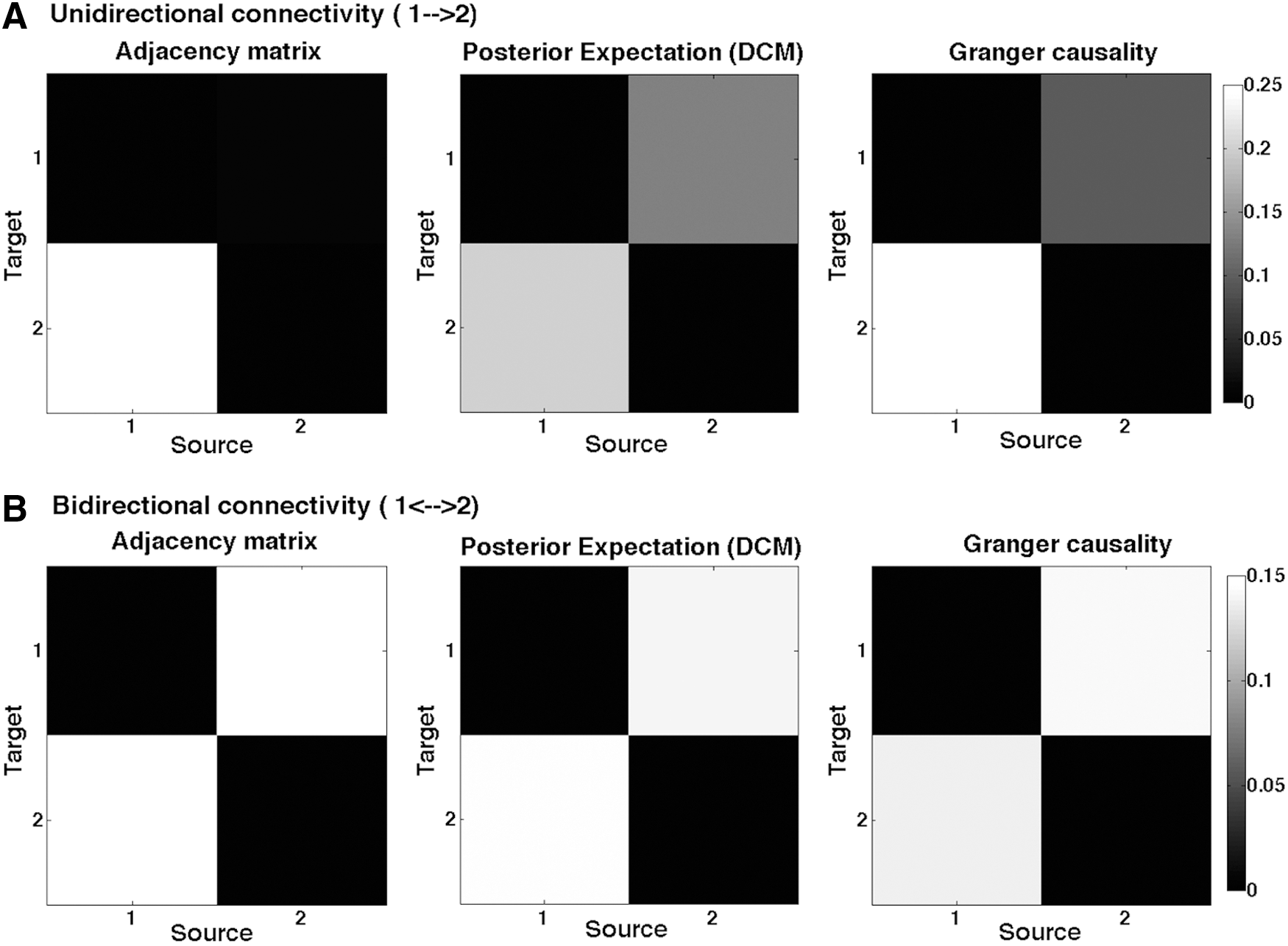
Connectivity between two sample nodes. (A) Asymmetric (unidirectional) and (B) symmetric (bidirectional) coupling between two nodes estimated from simulated time series data are shown. In this study, the adjacency matrices encoded the weighted coupling that provides a quantitative estimate of the directed functional or effective connectivity, posterior estimates (DCM) represent effective connectivity and GC matrices (calculated using nonparametric GC approach) represent directed functional connectivity. DCM, dynamic causal modeling; GC, Granger causality.

Figure 1 shows the connectivity or adjacency matrices that provide a quantitative estimate of the directed functional or effective connectivity. The posterior estimates from DCM represent effective connectivity, and the GC matrices represent directed functional connectivity between the nodes calculated using nonparametric GC. One can see that when data were simulated with asymmetric (unidirectional) coupling, both the DCM and GC estimates are asymmetric (with a greater connectivity from the first to the second node). Conversely, when connectivity was symmetric (reciprocal), both GC and DCM estimated the effective and functional connectivity to be the same in both directions.

GC: directed functional connectivity—empirical data

In the analysis of the empirical data, the in-degree for each node (from the remaining three nodes) was calculated using Equation (3). Figure 2 shows the total in-degree for each node, integrated over the frequency band 0.0021–0.1 Hz, averaging over all the trials (subjects and voxels combined). We found the minimum in-degree for mPFC (R2) and the maximum for LAG (R4) in the order: LAG (R4)>PCC (R1)>LMTC (R3)>mPFC (R2).

FIG. 2.

GC analysis: In-degree for each of the four ROIs. Total in-degree, calculated from GC analysis, for each region is shown from the other three regions in ascending order. ROIs, regions of interest.

DCM: effective connectivity–empirical data

Five models were compared using DCM, where the “optimal” model was identified using BMS. Models were based on the anatomical connections with established literature (model: 1) and the in-degree obtained from nonparametric GC approach (models: 2–5) (Fig. 3). In this study, model-1 represents bidirectional connections among all the nodes, whereas models 2–5 represent total in-degree [LAG (R4) (model-2)>PCC (R1) (model-3)>LMTC (R3) (model-4)>mPFC (R2) (model-5)] in the same order suggested by the GC analysis (Fig. 2). Using RFX-BMS approach, we found that model-1 was the winning model and model-2 was the second best model (Fig. 4). This suggested that there are direct projections to LAG (R4) from the remaining regions. This was consistent with GC, where we obtained the greatest in-degree for LAG (R4) (Fig. 2).

FIG. 3.

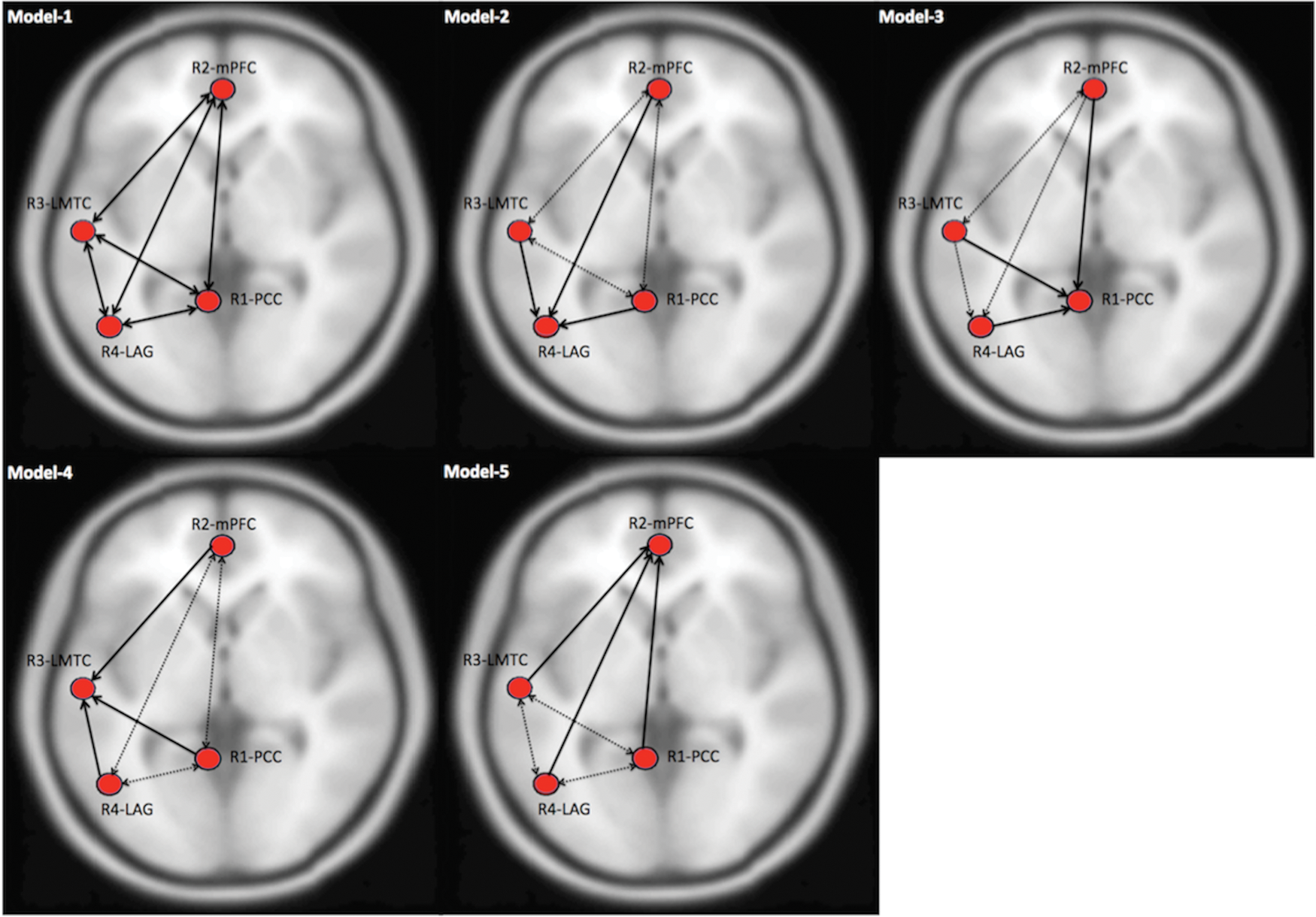
Defining a model space for DCM analysis. A base-model (model-1) is defined on the basis of anatomical connections (shown with solid lines) among the four ROIs, whereas models (2–5) are based on in-degree values calculated from GC analysis. In this study, LAG (R4) has the maximum in-degree (model-2), followed by PCC (R1) (model-3), LMTC (R3) (model-4), and mPFC (R2) (model-5), shown with solid lines, whereas anatomical connections in models 2–5 are shown with dashed lines. LMTC, left middle temporal cortex; mPFC, medial prefrontal cortex; PCC, posterior cingulate cortex. LAG, left angular gyrus. Color images available online at www.liebertpub.com/brain

FIG. 4.

Model expected and model exceedance probability. Model expected probability and model exceedance probability for five models are calculated using RFX-BMS approach in DCM. In this study, base model (model-1) is the winning model that shows maximum model exceedance probability of 78%, whereas the second best model (model-2) shows model exceedance probability of 22% verifying maximum in-degree for LAG (R4). RFX-BMS, random effects Bayesian model selection.

GC versus DCM—a comparative evaluation

The total in-degree for each node was compared to the average afferent connectivity for each node following BMA, averaging over all the subjects (Fig. 5A) and considering the subject-specific values for each node (Fig. 5B). Although we found higher in-degree for LMTC relative mPFC (whereas connectivity strength for LMTC was lower than mPFC), the results in Figure 5A suggest that a higher (GC) in-degree for a node is associated with a stronger (BMA) connection to that node and vice versa. This is further confirmed in Figure 5B, which shows a positive significant linear relationship (r = 0.38, p < 0.01) between the two directed connectivity measures, when subject-specific measures are taken into account.

FIG. 5.

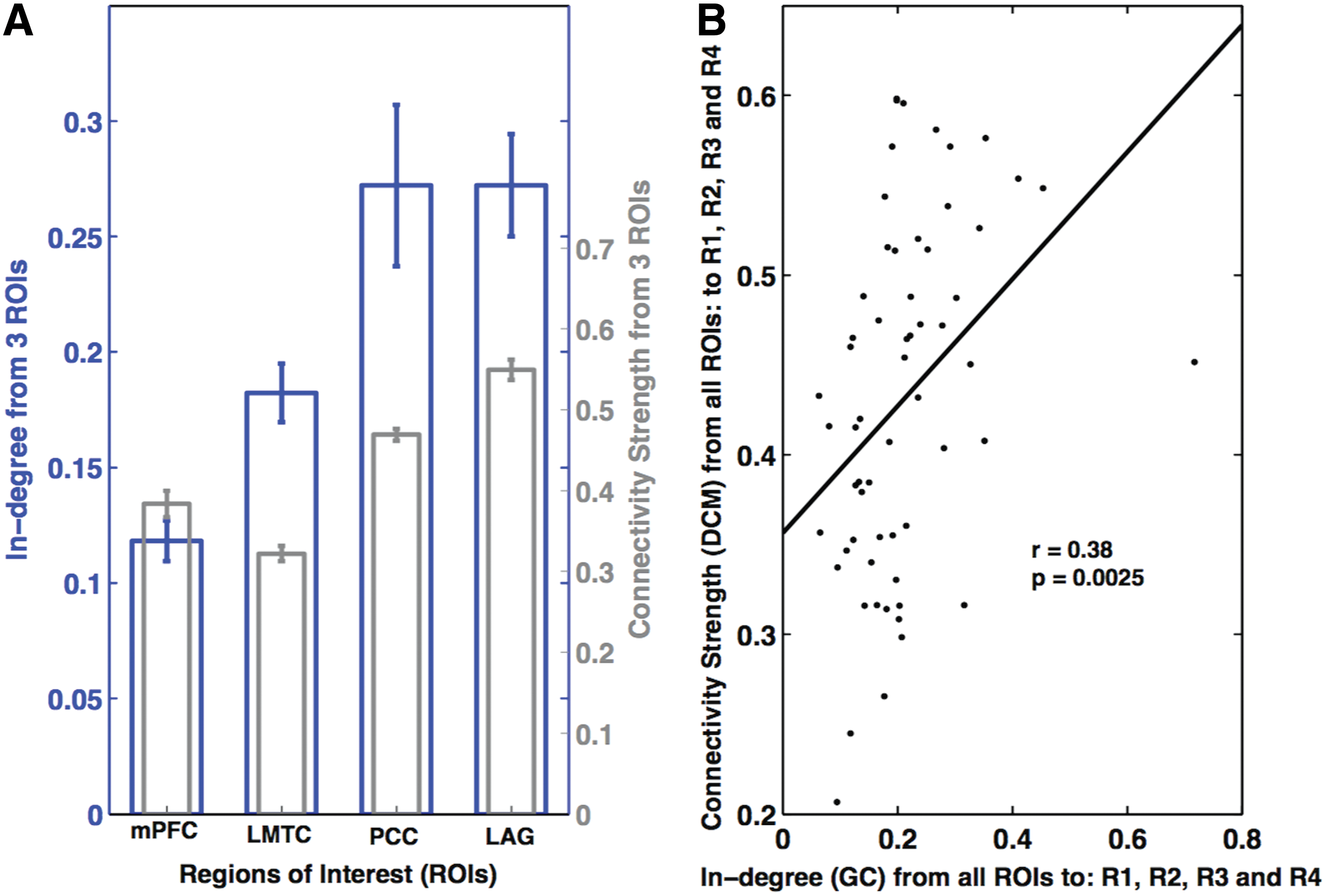
Explicit comparison of in-degree values obtained from GC and connectivity strength parameters obtained from DCM. (A) Total in-degree for each region, averaged over all the subjects and over the frequency interval 0.0021–0.1 Hz, is compared to average afferent connection strength for corresponding region, averaged over all the subjects. In this study, error bars represent standard error of mean. (B) A significant positive linear relationship (r = 0.38, p = 0.0025) is found between the two measures of afferent connectivity over the four nodes from each subject. Color images available online at www.liebertpub.com/brain

Discussion

In the current report, we investigated the directed coupling between two regions by modeling synthetic data (Friston et al., 2010). We obtained consistent inferences about directed connections, when we applied a nonparametric GC scheme and DCM to the synthetic data. Furthermore, using resting state MRI data, we computed Granger causal connectivity within the DMN comprising four regions (PCC, mPFC, LMTC, and LAG), which are anatomically connected. We estimated effective connectivity among these regions by defining a model space using DCM and compared average (afferent) connectivity to the total in-degree for each node obtained from GC approach. The winning model structure and Bayesian parameter averages (obtained from BMS) and the in-degree measures obtained from GC were found to be consistent. In addition, the connectivity from BMA was significantly correlated with directed functional connectivity values obtained from GC. Note that we did not assume that an asymmetry in GC means that a connection in the DCM is unidirectional. We simply considered the possibility that some directed connections could be zero by including (reduced) models in our model space—and then averaged over models using BMA. This accommodates a degree of uncertainty about the architecture generating the data. To our knowledge, these are new findings that speak to the convergence of GC and DCM and offer a degree of construct validity to both (Friston, 2011a, 2013; Mahroos and Kadah, 2011; Valdes-Sosa et al., 2011).

To redress face validity of both schemes, we used synthetic data, where we knew the underlying connectivity architecture. Using these simulated data, we found that both GC and DCM could recover the asymmetric (unidirectional) and symmetric (reciprocal) connectivity used to generate the data. Note that we simulated data, using the same sort of (DCM) model that was used for estimating effective connectivity. One might think that a more balanced test of the ability of DCM and GC to recover directed effective and functional connectivity might entail simulating data using models based upon DCM and GC, and then using both procedures to infer coupling with both sorts of simulated data. However, this is not possible, because the models underlying GC (especially nonparametric models) are not generative models. In other words, GC does not provide a model that can be used to generate data. Although one can generate time series using an AR process—of the sort used in GC—the implicit regression model simply describes dependencies among observed data. This is fundamentally different from having a forward or generative model that generates observed data from latent or hidden neuronal states.

Mathematically, this means that although one can always derive the AR equivalent of a time series generated by a DCM, it is not possible to uniquely identify the underlying (effective) connectivity that generated the AR coefficients. A fuller discussion of this can be found in Friston et al. (2014a) and Valdes-Sosa et al. (2011). In practice, this means that the only way to generate plausible fMRI time series is to use a DCM-like model to produce correlated observations—and then proceed (as we have above) by inferring the coupling in terms of parameter estimates; namely, the effective connectivity for DCM and the autoregression coefficients (or spectral equivalents) for GC. Granger causality then rests upon an implicit form of Bayesian model comparison—comparing models with and without particular coefficients. This model comparison is similar to the model comparison used by DCM, when trying to identify particular architectures. This highlights a further fundamental difference between measures of coupling using GC and DCM: the measures in GC pertain to the significance of directed functional connectivity—as assessed by comparing models with and without a particular dependency; whereas the estimated connectivity DCM is a quantitative measure of the coupling strength.

Furthermore, from empirical data analysis, we found that—within DMN—the directionality obtained from DCM analysis was consistent with the directionality obtained from GC. Both the approaches showed that LAG was subjected to the largest influences from other areas, with decreasing influences on PCC, LMTC, and the least on mPFC. We found a significant positive linear relationship between in-degree parameters and average connection strength parameters, considering values over all the subjects and nodes. Previous studies have illustrated the utility of GC and DCM for connectivity analysis, using simulated data as well as empirical fMRI/EEG data (Bressler and Seth, 2010; Friston et al., 2003; Li et al., 2011; Seth et al., 2013). Although none of the studies has compared the results of GC and DCM directly, some have discussed their integration (Friston et al., 2013; Mahroos and Kadah, 2011; Mitra and Pesaran, 1999; Valdes-Sosa et al., 2011).

In this study, we found that the first model was the winning model over other models, since these four areas are known to be connected to each other functionally as well as anatomically (Bajaj et al., 2013). Furthermore, model 2—with the maximum in-degree to LAG—was the second best model. This model, along with other models constituting the model space, was constructed by assuming that GC values reflect the directionality of coupling between the nodes.

GC is based on empirical observations, which enable the estimation of AR coefficients. We used the nonparametric GC approach in this study—instead of parametric approach that requires the proper determination of model order to balance variance and complexity and sometimes fails to capture complex data features (Dhamala et al., 2008b; Mitra and Pesaran, 1999). The application of GC to fMRI had been a topic of debate in recent years. Some studies have considered empirical and theoretical concerns regarding its application to fMRI data (Friston, 2009; Friston, 2011a; Zou and Feng, 2009). It has been suggested that GC cannot infer the true direction of the causal influences because of variability in the shape and latency of HRFs in different brain regions and different subjects (Aguirre et al., 1998; David et al., 2008; Schippers et al., 2011). However, a simulation study by Deshpande et al. (2010) found that GC was sufficiently flexible to accommodate hemodynamic variability. Bressler and Seth (2010) illustrated the applicability of GC to fMRI—showing GC can estimate causal statistical influences from simultaneously recorded neural time series data. Moreover, deconvolution of fMRI BOLD signals can be used to recover measures of the underlying neural processes (Aquino et al., 2014; David et al., 2008). Besides neural activity, various other factors such as slice timing differences, baseline cerebral blood flow, baseline hematocrit, hemodilution, alcoholic/lipid intakes, and different respiration rates across individuals are also responsible for HRF variability (Deshpande et al., 2010; Levin et al., 1998; Levin et al., 2001; Noseworthy et al., 2003). Furthermore, it was also found that lower sampling rates and noise could confound fMRI GC (Deshpande et al., 2010; Seth et al., 2013; Solo, 2007).

In the near future, because of advances in technology, it may be that concerns about lower sampling rate will not remain a major problem (Feinberg et al., 2010). Wen et al. (2013) addressed the effect of various factors such as (1) latency differences in HRF across brain areas, (2) low sampling rates, and (3) noise by linking fMRI GC and neural GC using simulated data. For TR = 2 sec and signal-to-noise ratio (SNR) = 5 (20% noise), they found a significant positive linear relationship (r = 0.96, p = 0) between the neural GC and fMRI GC in case of unidirectional coupling, but no correlation was found for reciprocal coupling. Interestingly, the correlation improved at higher sampling rates. This study is in agreement with other studies suggesting that the HRF had a less severe impact on GC calculations, whereas downsampling and noise can confound GC (Nalatore et al., 2007, 2009; Wen et al., 2013).

Hence, despite concerns regarding the use of GC with fMRI data, there are numerous studies available endorsing GC. We combined GC and DCM to compare both approaches, using the in-degree from GC as priors in the construction of a model space for DCM. Since DCM is well established for fMRI data—and we found an association between GC and DCM—the contribution of the current work is to establish their construct validity both in terms of model identification and quantitative estimation of directed coupling. Furthermore, we have illustrated how GC may provide useful constraints on the construction of model spaces or hypotheses that can be tested subsequently using DCM. We expect this work may address some previous concerns regarding connectivity analyses and contribute to the further study of distributed neuronal dynamics.

It should be acknowledged that the current results do not establish the criteria for a convergence between GC and DCM. They only provide proof of principle that convergence can be obtained under idealized settings; for example, the exceedingly long time series of the sort used in simulations. A formal analysis of the criteria for convergent results would entail a thorough analysis of the robustness and validity of both approaches under plausible assumptions of realistic synthetic data. Clearly, these are important (and outstanding) issues in their own right—irrespective of the construct facility we have tried to address. In summary, it might be better to regard the current report as a description of a protocol that can be used to assess the face and construct validity of GC and DCM, using simulated data. The future work should assess (1) how the convergence between the two approaches depends upon the data quality (signal-to-noise ratio, nonstationarity, strength of interactions), (2) how these two approaches compare in computation time for time series lengths and the size of the ROI, and (3) how the explicit connectivity changes in DCM relate to changes in GC estimates.

Conclusions

Using simulated data for two regions, we found that both directed functional connectivity and effective connectivity reflect asymmetries in the coupling between regions. Using empirical fMRI data, we found that an anatomically interconnected network of four nodes (PCC, mPFC, LMTC, LAG) was engaged during the resting state. Furthermore, we performed DCM analysis on this network, using GC to elaborate a hypothesis or model space. Directionality among the four regions reflected by the winning model obtained using BMS was consistent with the directed functional connectivity obtained from nonparametric GC. Furthermore, quantitatively, the positive correlation between connectivity obtained from BMA and in-degree parameters obtained from GC confirmed the consilience of both approaches for rsfMRI data. Future investigations of more complex data (e.g., task based and clinical) are required to generalize our construct validation of GC and DCM for fMRI data.

Footnotes

Acknowledgments

This work was supported by NSF CAREER Award (BCS 0955037) awarded to M. Dhamala. K.J.F. was supported by a Wellcome Trust Principal Research Fellowship (Ref: 088130/Z/09/Z). The authors would like to thank Dr. William Penny, Dr. Guillaume Flandin, and Dr. Klaas E. Stephan for their replies to our posts in SPM discussion forum (www.jiscmail.ac.uk) on numerous occasions.

Author Disclosure statement

No competing financial interests exist.

References

Aguirre

, Zarahn

, D'esposito

. 1998. The variability of human, BOLD hemodynamic responses. Neuroimage, 8:360–369.

Aquino

, Robinson

, Schira

, Breakspear

. 2014. Deconvolution of neural dynamics from fMRI data using a spatiotemporal hemodynamic response function. Neuroimage, 94:203–215.

Ashburner

, Friston

. 1999. Nonlinear spatial normalization using basis functions. Hum Brain Mapp, 7:254–266.

Bajaj

, Adhikari

, Dhamala

. 2013. Higher frequency network activity flow predicts lower frequency node activity in intrinsic low-frequency BOLD fluctuations. PLoS One, 8:e64466.

Bajaj

, Butler

, Drake

, Dhamala

. 2015. Functional organization and restoration of the brain motor-execution network after stroke and rehabilitation. Front Hum Neurosci, 9:1–14.

Bajaj

, Drake

, Butler

, Dhamala

. 2014. Oscillatory motor network activity during rest and movement: an fNIRS study. Front Syst Neurosci, 8:13.

Barrett

, Murphy

, Bruno

, Noirhomme

, Boly

, Laureys

, Seth

. 2012. Granger causality analysis of steady-state electroencephalographic signals during propofol-induced anaesthesia. PLoS One, 7:e29072.

Bastos

, Vezoli

, Bosman

, Schoffelen

, Oostenveld

, Dowdall

, et al. 2015. Visual areas exert feedforward and feedback influences through distinct frequency channels. Neuron, 85:390–401.

Bernasconi

, Konig

. 1999. On the directionality of cortical interactions studied by structural analysis of electrophysiological recordings. Biol Cybern, 81:199–210.

10.

Boly

, Moran

, Murphy

, Boveroux

, Bruno

M-A

, Noirhomme

, et al. 2012. Connectivity changes underlying spectral EEG changes during propofol-induced loss of consciousness. J Neurosci, 32:7082–7090.

11.

Bosman

, Schoffelen

, Brunet

, Oostenveld

, Bastos

, Womelsdorf

, et al. 2012. Attentional stimulus selection through selective synchronization between monkey visual areas. Neuron, 75:875–888.

12.

Bressler

, Seth

. 2010. Wiener-Granger causality: a well established methodology. Neuroimage, 58:323–329.

13.

Brovelli

, Ding

, Ledberg

, Chen

, Nakamura

, Bressler

. 2004. Beta oscillations in a large-scale sensorimotor cortical network: directional influences revealed by Granger causality. Proc Natl Acad Sci U S A, 101:9849–9854.

14.

Chang

, Glover

. 2010. Time-frequency dynamics of resting-state brain connectivity measured with fMRI. Neuroimage, 50:81–98.

15.

David

, Guillemain

, Saillet

, Reyt

, Deransart

, Segebarth

, Depaulis

. 2008. Identifying neural drivers with functional MRI: an electrophysiological validation. PLoS Biol, 6:2683–2697.

16.

Deco

, Jirsa

, Robinson

, Breakspear

, Friston

. 2008. The dynamic brain: from spiking neurons to neural masses and cortical fields. PLoS Comput Biol, 4:e1000092.

17.

Deshpande

, Sathian

, Hu

. 2010. Effect of hemodynamic variability on Granger causality analysis of fMRI. Neuroimage, 52:884–896.

18.

Dhamala

. 2015. Spectral interdependency methods. In: Jaeger

, Jung

(eds.) Encyplopedia of Computational Neuroscience. New York, NY: Springer, pp. 2789–2793.

19.

Dhamala

, Rangarajan

, Ding

. 2008a. Analyzing information flow in brain networks with nonparametric Granger causality. Neuroimage, 41:354–362.

20.

Dhamala

, Rangarajan

, Ding

. 2008b. Estimating Granger causality from Fourier and wavelet transforms of time series data. Phys Rev Lett, 100:018701.

21.

Ding

, Bressler

, Yang

, Liang

. 2000. Short-window spectral analysis of cortical event-related potentials by adaptive multivariate autoregressive modeling: data preprocessing, model validation, and variability assessment. Biol Cybern, 83:35–45.

22.

Ding

, Chen

, Bressler

. 2006. Granger Causality: Basic Theory and Application to Neuroscience. Wienheim: Wiley.

23.

Feinberg

, Moeller

, Smith

, Auerbach

, Ramanna

, Glasser

, et al. 2010. Multiplexed echo planar imaging for sub-second whole brain FMRI and fast diffusion imaging. PLoS One, 5:e15710.

24.

Fox

, Zhang

, Snyder

, Raichle

. 2009. The global signal and observed anticorrelated resting state brain networks. J Neurophysiol, 101:3270–3283.

25.

Friston

. 2011a. Dynamic causal modeling and Granger causality comments on: the identification of interacting networks in the brain using fMRI: model selection, causality and deconvolution. Neuroimage, 58:303–305.

26.

Friston

. 2011b. Functional and effective connectivity: a review. Brain Connect, 1:13–36.

27.

Friston

, Harrison

, Penny

. 2003. Dynamic causal modelling. Neuroimage, 19:1273–1302.

28.

Friston

, Moran

, Seth

. 2013. Analysing connectivity with Granger causality and dynamic causal modelling. Curr Opin Neurobiol, 23:172–178.

29.

Friston

, Penny

. 2011. Post hoc Bayesian model selection. Neuroimage, 56:2089–2099.

30.

Friston

, Stephan

, Li

, Daunizeau

. 2010. Generalised filtering. Math Probl Eng, 2010:1–34.

31.

Friston

. 1994. Functional and effective connectivity in neuroimaging: a synthesis. Hum Brain Mapp, 2:56–78.

32.

Friston

. 2009. Causal modelling and brain connectivity in functional magnetic resonance imaging. PLoS Biol, 7:220–225.

33.

Friston

, Bastos

, Oswal

, van Wijk

, Richter

, Litvak

. 2014a. Granger causality revisited. Neuroimage, 101:796–808.

34.

Friston

, Kahan

, Biswal

, Razi

. 2014b. A DCM for resting state fMRI. Neuroimage, 94:396–407.

35.

Geweke

. 1982. Measurement of linear dependence and feedback between multiple time series. J Am Statist Assoc, 77:304–313.

36.

Geweke

. 1984. Measures of conditional linear dependence and feedback between time series. J Am Statist Assoc, 79:907–915.

37.

Granger

CWJ

. 1969. Investigating causal relations by econometric models and cross-spectral methods. Econometrica, 37:424–438.

38.

Kim

, Putrino

, Ghosh

, Brown

. 2011. A Granger causality measure for point process models of ensemble neural spiking activity. PLoS Comput Biol, 7:e1001110.

39.

Levin

, Frederick

, Ross

, Fox

, von Rosenberg

, Kaufman

, et al. 2001. Influence of baseline hematocrit and hemodilution on BOLD fMRI activation. Magn Reson Imaging, 19:1055–1062.

40.

Levin

, Ross

, Mendelson

, Kaufman

, Lange

, Maas

, et al. 1998. Reduction in BOLD fMRI response to primary visual stimulation following alcohol ingestion. Psychiatry Res, 82:135–146.

41.

, Daunizeau

, Stephan

, Penny

, Hu

, Friston

. 2011. Generalised filtering and stochastic DCM for fMRI. Neuroimage, 58:442–457.

42.

Liu

, Duyn

. 2013. Time-varying functional network information extracted from brief instances of spontaneous brain activity. Proc Natl Acad Sci U S A, 110:4392–4397.

43.

Mahroos

, Kadah

. 2011. Brain causality investigation based on FMRI images time series using dynamic causal modelling augmented by Granger causality. In: National Radio Science Conference (NRSC) Egypt.

44.

Mitra

, Pesaran

. 1999. Analysis of dynamic brain imaging data. Biophys J, 76:691–708.

45.

Nalatore

, Ding

, Rangarajan

. 2007. Mitigating the effects of measurement noise on Granger causality. Phys Rev E Stat Nonlin Soft Matter Phys, 75:031123.

46.

Nalatore

, Ding

, Rangarajan

. 2009. Denoising neural data with state-space smoothing: method and application. J Neurosci Meth, 179:131–141.

47.

Noseworthy

, Alfonsi

, Bells

. 2003. Attenuation of brain BOLD response following lipid ingestion. Hum Brain Mapp, 20:116–121.

48.

Penny

, Stephan

, Daunizeau

, Rosa

, Friston

, Thomas

, Leff

. 2010. Comparing families of dynamic causal models. PLoS Comput Biol, 6:1000709.

49.

Roebroeck

, Formisano

, Goebel

. 2011. The identification of interacting networks in the brain using fMRI: model selection, causality and deconvolution. Neuroimage, 58:296–302.

50.

Schippers

, Renken

, Keysers

. 2011. The effect of intra- and inter-subject variability of hemodynamic responses on group level Granger causality analyses. Neuroimage, 57:22–36.

51.

Seth

, Chorley

, Barnett

. 2013. Granger causality analysis of fMRI BOLD signals is invariant to hemodynamic convolution but not downsampling. Neuroimage, 65:540–555.

52.

Solo

. 2007. On causality I: sampling and noise. In: Proceedings of the 46th IEEE Conference on Decision and Control. December, 12–14, 2007, New Orleans, LA, pp. 3634–3639.

53.

Stephan

, Penny

, Daunizeau

, Moran

, Friston

. 2009. Bayesian model selection for group studies. Neuroimage, 46:1004–1017.

54.

Stephan

, Penny

, Moran

, den Ouden

, Daunizeau

, Friston

. 2010. Ten simple rules for dynamic causal modeling. Neuroimage, 49:3099–3109.

55.

Stephan

, Weiskopf

, Drysdale

, Robinson

, Friston

. 2007. Comparing hemodynamic models with DCM. Neuroimage, 38:387–401.

56.

Talairach

, Tournoux

. 1988. Co-planar Stereotaxic Atlas of the Human Brain. New York: Thieme Medical.

57.

Valdes-Sosa

, Roebroeck

, Daunizeau

, Friston

. 2011. Effective connectivity: influence, causality and biophysical modeling. Neuroimage, 58:339–361.

58.

Wen

, Rangarajan

, Ding

. 2013. Is Granger causality a viable technique for analyzing fMRI data?. PLoS One, 8:e67428.

59.

Zou

, Feng

. 2009. Granger causality vs. dynamic Bayesian network inference: a comparative study. BMC Bioinformatics, 10:122.