Graph Theory at the Service of Electroencephalograms

Abstract

The brain is one of the largest and most complex organs in the human body and EEG is a noninvasive electrophysiological monitoring method that is used to record the electrical activity of the brain. Lately, the functional connectivity in human brain has been regarded and studied as a complex network using EEG signals. This means that the brain is studied as a connected system where nodes, or units, represent different specialized brain regions and links, or connections, represent communication pathways between the nodes. Graph theory and theory of complex networks provide a variety of measures, methods, and tools that can be useful to efficiently model, analyze, and study EEG networks. This article is addressed to computer scientists who wish to be acquainted and deal with the study of EEG data and also to neuroscientists who would like to become familiar with graph theoretic approaches and tools to analyze EEG data.

Introduction

The human brain is probably one of the most complex structures in nature and unraveling its mysteries constitutes maybe one of the greatest challenges faced by 21st century science. No other brain in the known universe is capable of generating the kind of higher and impressive consciousness that is associated with human ingenuity. Toward that direction, the Human Brain Project (Europe^* and USA^†), which is a large 10-year scientific research project, aims exactly at simulating the complete human brain to better understand how it functions. To accomplish these goals, both continental projects collect, analyze, and model consistent recording of brain data sets and employ network science methods supported by brain theory, since all brain networks can be characterized by neurobiologically meaningful graph theory metrics (Bullmore and Sporns, 2009; Joudaki et al., 2012; Sporns, 2013).

The term brain connectivity refers to several different and interrelated aspects of brain organization. A fundamental distinction is between structural connectivity, functional connectivity, and effective connectivity (Friston, 1994). Anatomical connectivity refers to a network of physical or structural (synaptic) connections linking sets of neurons or neuronal elements, as well as their associated structural biophysical attributes encapsulated in parameters such as synaptic strength or effectiveness. Functional connectivity, in contrast, is fundamentally a statistical concept. In general, functional connectivity captures deviations from statistical independence between distributed and often spatially remote neuronal units. Finally, effective connectivity may be viewed as the union of structural and functional connectivity, as it describes networks of directional effects of one neural element over another. In this article, we mainly focus on EEG functional connectivity networks, because they are the most commonly used ones.

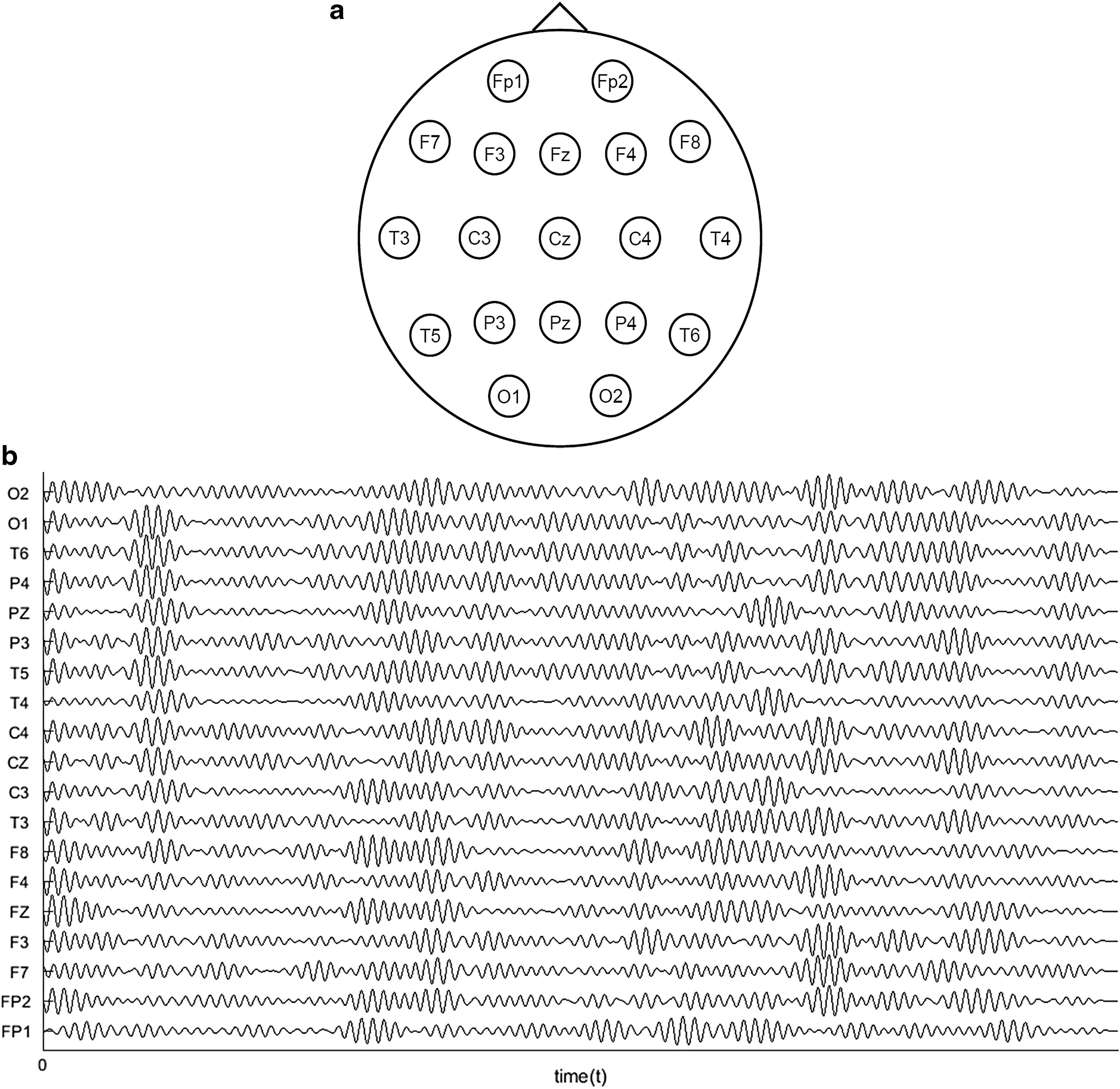
One of the most widely used methods to measure and record the electrical activity of the brain worldwide is the EEG, which uses special sensors (electrodes) that are placed in specific areas along the scalp and each one of them records a space average of cortical source activity, as shown in Figure 1a. Also, the sizes of cortical regions contributing to each electrode depend on whether untransformed or high resolution EEG (e.g., spline-Laplacian) is studied. The name of each electrode (e.g., Cz, F4, and P3) is unique in each recording and denotes its position on the scalp. These electrodes detect tiny electrical charges that result from the activity of the brain cells (Niedermeyer et al., 2012). The charges are amplified and appear most of the times as a recording signal that may be printed out on a paper or a computer screen (Fig. 1b). Basic parameters in a recording procedure constitute the total number of electrodes, the sampling frequency (or sampling rate), and the bit resolution. EEG recording data also include meta-data, which are mainly markers that usually have the form, <name, value>. These markers are indicated by experts to note events of interest, which could be, for example, epileptic seizures, spikes, encephalopathies, or sleep spindles. An event of interest can be described from one or more markers. For instance, we can use two markers for an epileptic seizure, the first to point out the start and the second to denote the end of it (Abou-Khalil and Misulis, 2006).

FIG. 1.

(a) Electrodes that are placed in specific areas along the scalp. (b) Example of an electroencephalogram recording.

EEGs present high research and clinical interest and they are widely used both in health and disease, for example, in diagnosing neurological disorders (Niedermeyer et al., 2012). This happens because measurements of brain electrical activity with EEG have long been one of the most valuable sources of information for research and diagnosis, since they carry a large amount of rich information and can be recorded continuously and over long periods of time (Iasemidis, 2011). They also present several advantages against other technologies (functional magnetic resonance imaging or magnetoencephalography) such as higher temporal resolution, lower price, and tolerance to movement. An EEG can provide information about possible abnormal electrical activity in the brain and in some cases the types of seizures that a person might be going through. The word “seizure” is generally used to describe a temporary change in the electrical activity of the brain (e.g., epileptic seizure) (Stump, 2008). One of the most common EEG applications is to show the type and location of the activity in the brain during a seizure. This information can then be used for making the right diagnosis. Beside seizures, an EEG is also used to evaluate people who have problems associated with brain functions, which might include, for example, coma, problems with memory, sleep disorders, tumors, encephalopathy (a disease that causes brain dysfunction), or weakness of specific body parts (such as weakness caused by a stroke). An EEG can also be used to determine brain death (Teplan, 2002).

In the past years, EEG data were mainly studied as signals and several methods to analyze brain function from these recordings have been proposed. They range from traditional linear methods, such as Fourier transforms and spectral analysis (Greenfield et al., 2010), to nonlinear methods derived from the theory of nonlinear dynamical systems, also called chaos theory (Pritchard and Duke, 1995; Stam, 2005). In general, chaos-based approaches outperform the traditional linear methodologies (Rabinovich et al., 2006), which assume that the signal is stationary and originates from a low-dimensional linear system. However, in reality, this is not always the case because a real EEG is a nonstationary signal (Gribkov and Gribkova, 2000). Moreover, given that EEGs are recorded continuously and many times over long periods of time, this often leads to the production of vast amount of data and makes the task of knowledge discovery from them quite difficult, but at the same time challenging as well. It is thus very important to develop new methods to study EEG signals in different physiological and pathological states.

EEGs are spatiotemporal data; since electrodes are placed on specific locations on the scalp and record continuously the electrical activity of the brain, we need new methods that will exploit both the spatial and temporal nature of these data. A basic precondition for the exportation of useful information from spatiotemporal data is the purposeful representation and description of EEG data using the appropriate techniques that maintain all the initial information and foster the application of data mining methodologies (del Mondo et al., 2013). For these reasons, recently, there has been a focus on studying EEG signals as graphs (networks) (Christodoulakis et al., 2012; Dimitriadis et al., 2012; Iakovidou et al., 2013a,b; Rubinov and Sporns, 2010) and in particular, there exists a growing interest in the theoretical aspects of network analysis in an attempt to model (Simpson et al., 2012; Vertes et al., 2012), describe (Rubinov and Sporns, 2010), and propose new measures (Joyce et al., 2010) for a better understanding of complex systems, such as the human brain.

A graph is a structure that consists of a set of vertices (or nodes) and a set of lines called edges that connect the nodes with each other. In case of EEG graphs, usually, each node corresponds to a particular electrode or pairs of electrodes and each edge corresponds to the connectivity estimates between different nodes (Fig. 2) (Dimitriadis et al., 2010). Generally, the graphs that are used to model the EEG spatiotemporal data can be divided in two categories (Brunet et al., 2011; de Pasquale et al., 2015; Iakovidou et al., 2013b): (i) static graphs, which represent connectivity estimates that correspond to a person's brain activity summarizing long recording periods (e.g., 8 sec) and (ii) time-varying graphs that represent a time series of connectivity estimates with each connectivity snapshot corresponding to a person's brain activity lasting for few milliseconds.

FIG. 2.

An example of complete and undirected EEG graph.

After having given a short overview of how EEG data can be modeled using graphs, we further emphasize on the computational analysis as defined in graph theory. The next section provides some basic concepts of graph theory using mathematical descriptions with regard to EEGs. Basic EEG Recording Properties and Construction of Brain Networks section presents some basic EEG recording properties and data processing regarding EEG brain network construction. Data Structures section describes the two main data structures that are used to represent and store EEG graph data. The next two sections further emphasize on the computational analysis of EEG graphs, by exploring different network properties and measures with regard to EEG brain networks. Finally, this article concludes providing a Discussion section.

Basic Graph Theory Definitions and Terms

To introduce the basic concepts of graph theory, we give both the empirical and the mathematical description of graphs that represent brain EEG networks as they are originally defined in the literature (Cohen and Havlin, 2010; Cormen et al., 2009; Niedermeyer et al., 2012).

An undirected graph is a structure that consists of a set of vertices (or nodes) and a set of lines called edges that connect the nodes with each other. Generally, a graph is symbolized as G = (V, E), where V is the set of vertices representing the nodes and E is the set of edges representing the connections between the nodes. We define as E = {(i, j) | i, j ∈ V} the single connection between nodes i and j, and consequently, we say that nodes i and j are neighbors.

On the other hand, a directed graph is defined as an ordered triple G = (V, E, f), where V is a nonempty set of vertices, E is a set of edges, and f is a function that associates each element in E with an ordered pair of vertices in V. The ordered pairs of vertices are called directed edges, arcs, or arrows and every edge E = (i, j) is considered to have direction from i to j.

In EEG graphs, each node corresponds to a particular electrode or pairs of electrodes and each edge corresponds to the connectivity estimates between different nodes. Every node is labeled differently, but not arbitrarily since it takes its name by the position that the electrodes have on the scalp. All EEG graphs are undirected and complete (fully connected), which means that every pair of distinct vertices is connected by a unique edge (Fig. 2). Another characteristic of EEG graphs is the fact that they are weighted (Rubinov and Sporns, 2010).

A weighted graph is defined as a graph G = (V, E) where V is a set of vertices and E is a set of edges between the vertices, E = {(u, v) | u, v ∈ V} associated with a weight function w: E → R, where R denotes the set of all real numbers. Most of the times, the weight w_ij of the edge between nodes i and j represents the relevance of the connection and this is true for EEG graphs, because a larger weight corresponds to higher reliability of a connection, as shown in Figure 3a. Many recent studies discard link weights and create binarized EEG graphs, where binary links denote just the presence or absence of connections (Fig. 3b), contrary to weighted links that contain information about connection strengths. Binary networks are in most cases simpler to study and have a more easily defined null model for statistical comparison. They can be used to improve visualization of a network or extract its main structure and they also constitute a preprocessing step for many data mining algorithms (Zhou et al., 2012). On the other hand, weighted characterization usually focuses on somewhat different and complementary aspects of network organization (Saramaki et al., 2007) and may be especially useful in filtering the influence of weak and potentially nonsignificant links.

FIG. 3.

(a) A weighted, undirected, and fully connected EEG graph. (b) The pruned and binarized version of (a). Color images available online at www.liebertpub.com/brain

If G = (V, E) is a graph, then G ₁ = (V ₁, E ₁) is called a subgraph of G if V ₁ ⊆ V and E ₁ ⊆ E, where each edge in E ₁ is incident with vertices in V ₁. In case of EEG graphs, a pruned graph of G, denoted by P(G), is a subgraph of G and can be obtained from it by deleting the least important edges (Zhou et al., 2012) according to a predefined procedure or threshold (Fig. 3b). This happens because weak and nonsignificant links may represent spurious connections and these links tend to obscure the topology of strong and significant connections. As a result, they are often discarded by applying an absolute or a proportional weight threshold. Threshold values are often arbitrarily determined, and networks should ideally be characterized across a broad range of thresholds (Rubinov and Sporns, 2010).

The degree k_i of a node i in an undirected graph is the number of other nodes in the graph to which node i is connected (or equivalently the number of edges adjacent to i) and it is defined as k_i = N(i), where N(i) is the number of neighbors of node i. The degree measurement has a straightforward neurobiological interpretation: nodes with a high degree are interacting, structurally or functionally, with many other nodes in the network. The average degree among all nodes in the network gives a picture of how well connected the graph is.

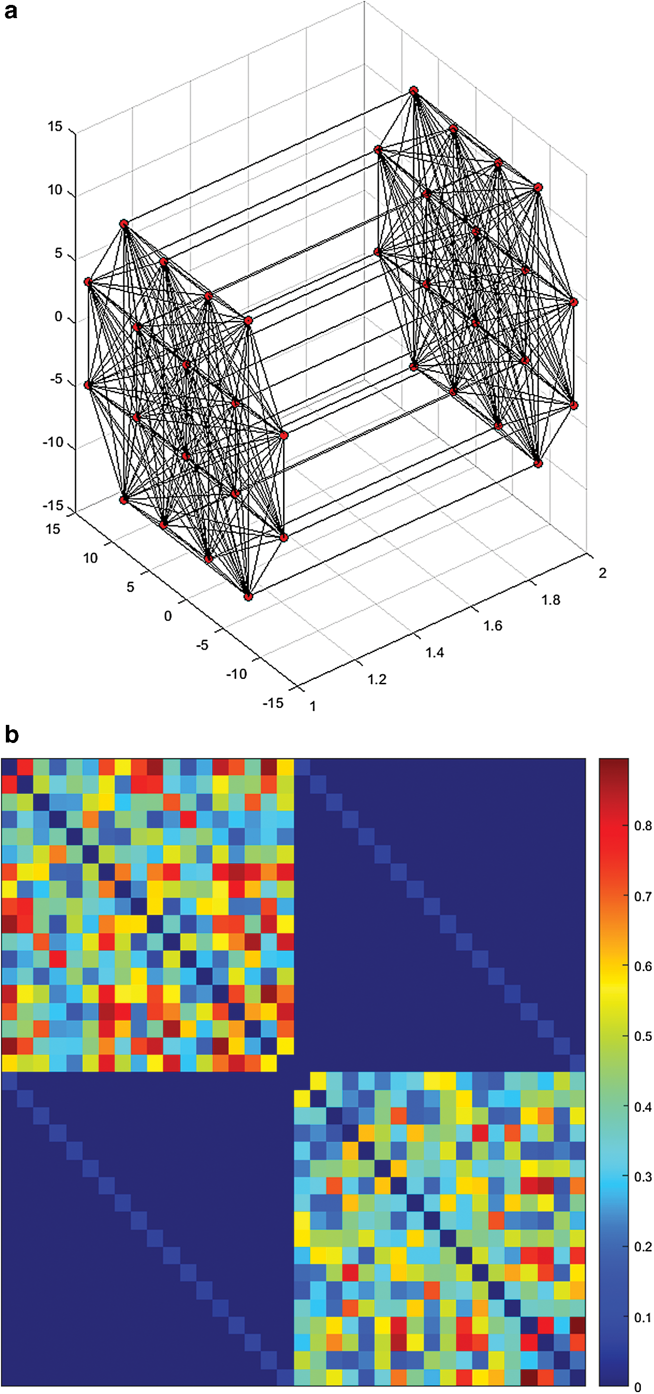
The network density is defined as \documentclass{aastex}\usepackage{amsbsy}\usepackage{amsfonts}\usepackage{amssymb}\usepackage{bm}\usepackage{mathrsfs}\usepackage{pifont}\usepackage{stmaryrd}\usepackage{textcomp}\usepackage{portland, xspace}\usepackage{amsmath, amsxtra}\usepackage{upgreek}\pagestyle{empty}\DeclareMathSizes{10}{9}{7}{6}\begin{document}$$C = \frac { E } { { N \left( { N - 1 } \right) } } $$ \end{document} , where E is the number of edges and N the total number of nodes. In a fully connected EEG graph, the total connectivity is always equal to 1 and the degree of every node is equal to N − 1.

A new concept for representing EEG data constitutes the idea of multislice networks. According to this, a given temporal sequence of weighted graphs (slices) corresponding to certain time-indexed connectivity snapshots is transformed into a single weighted graph, which contains all the slices connected together and corresponds to a multislice network (Fig. 4). In particular, borrowing the concept form a recent work on time-varying graphs (Cardillo et al., 2014), which introduced a measure that expresses the tendency of the edges to persist over time, the following quantity is assigned as weight to the link connecting node i over two consecutive network slices, indexed by t and t + 1: \documentclass{aastex}\usepackage{amsbsy}\usepackage{amsfonts}\usepackage{amssymb}\usepackage{bm}\usepackage{mathrsfs}\usepackage{pifont}\usepackage{stmaryrd}\usepackage{textcomp}\usepackage{portland, xspace}\usepackage{amsmath, amsxtra}\usepackage{upgreek}\pagestyle{empty}\DeclareMathSizes{10}{9}{7}{6}\begin{document} \begin{align*} \gamma _ { \left[ { t , t \, + 1 } \right] } ^i = { \frac { \sum \nolimits_j w_ { ij } ^ { \,t } w_ { ij } ^ { \,t + 1 } } { \sqrt { s_i^ts_i^ { t + 1 } } } } \end{align*} \end{document}

where \documentclass{aastex}\usepackage{amsbsy}\usepackage{amsfonts}\usepackage{amssymb}\usepackage{bm}\usepackage{mathrsfs}\usepackage{pifont}\usepackage{stmaryrd}\usepackage{textcomp}\usepackage{portland, xspace}\usepackage{amsmath, amsxtra}\usepackage{upgreek}\pagestyle{empty}\DeclareMathSizes{10}{9}{7}{6}\begin{document}$$w_{ij}^t$$ \end{document} are the elements of the weighted adjacency matrix of the time-varying graph at snapshot t and \documentclass{aastex}\usepackage{amsbsy}\usepackage{amsfonts}\usepackage{amssymb}\usepackage{bm}\usepackage{mathrsfs}\usepackage{pifont}\usepackage{stmaryrd}\usepackage{textcomp}\usepackage{portland, xspace}\usepackage{amsmath, amsxtra}\usepackage{upgreek}\pagestyle{empty}\DeclareMathSizes{10}{9}{7}{6}\begin{document}$$s_i^t$$ \end{document} is the strength of node i at snapshot t. An example of a multislice graph is depicted in Figure 4a. This particular example contains two slices that correspond to two different time snapshots t and t + 1. The red color edges are the ones that were added according to the aforementioned procedure, to create the multislice graph. The potential of this approach stems from the fact that the constructed multislice network encompasses both temporal and spatial characteristics of EEG networks. Also, the characterization of that kind of networks, using standard network metrics, such as those presented in Network Properties and Network Topology and Measures sections, offers new possibilities in understanding the self-organization trends and behavior of EEGs (Tang et al., 2010). There are other studies that also use the aforementioned approach to detect, for example, community organization of brain connectivity over time (Bassett et al., 2011) or to evaluate dynamics of the cerebral networks during the execution of the foot movement (De Vico Fallani et al., 2008a).

FIG. 4.

(a) A simple representative example of a multislice network. (b) The weighted adjacency matrix of the multislice network shown in (a). Links in red depict the weights of the inter-slice links. Color images available online at www.liebertpub.com/brain

Basic EEG Recording Properties and Construction of Brain Networks

As mentioned before, the electroencephalogram is a recording of the electrical activity of the brain from the scalp and its recorded waveforms reflect the cortical electrical activity. EEG activity is quite small, so the signal intensity is measured in microvolts and the main signal frequencies of the human EEG waves are as follows (Kramarenko and Tan, 2003; Nunez and Srinivasan, 2006a,b):

• Delta: Has a frequency of 3 Hz or below. It tends to be the highest in amplitude and the one with slowest waves. It is normal as the dominant rhythm in infants up to 1 year and in stages 3 and 4 of sleep. It may occur focally with subcortical lesions and in general distribution with diffuse lesions, metabolic encephalopathy hydrocephalus, or deep midline lesions. It is usually most prominent frontally in adults (e.g., FIRDA—frontal intermittent rhythmic delta) and posteriorly in children (e.g., OIRDA—occipital intermittent rhythmic delta) (Brigo, 2011).

• Theta: Has a frequency of 3.5–7.5 Hz and is classified as “slow” activity. It is perfectly normal in children up to 13 years and in sleep, but abnormal in awake adults. It can be seen as a manifestation of focal subcortical lesions. It can also be seen in generalized distribution in diffuse disorders such as metabolic encephalopathy or some instances of hydrocephalus. This range has been also associated with reports of relaxed and meditative states (Cahn and Polich, 2006).

• Alpha: Has a frequency between 7.5 and 13 Hz. It is usually best seen in the posterior regions of the head on each side, being higher in amplitude on the dominant side. It appears when closing the eyes and relaxing, and disappears when opening the eyes or alerting by any mechanism (thinking, calculating). It is the major rhythm seen in normal relaxed adults and is present during most of life, especially after the 13th year. Alpha can also be abnormal, for example, an EEG that has diffuse alpha occurring in coma and is not responsive to external stimuli is referred to as alpha “coma” (Niedermeyer, 1997).

• Beta: Beta activity is “fast” activity. It has a frequency of 14 and greater Hz (up to 28 Hz). It is usually seen on both sides in symmetrical distribution and is most evident frontally. It is accentuated by sedative–hypnotic drugs, especially the benzodiazepines and the barbiturates. It may be absent or reduced in areas of cortical damage. It is generally regarded as a normal rhythm and is the dominant rhythm in patients who are alert or anxious, or have their eyes open (Pfurtscheller and Lopes Da Silva, 1999).

• Gamma: Gamma waves have a frequency between 25 and 100 Hz, although 40 Hz is typical (Gold, 1999). Gamma waves were initially ignored before the development of digital electroencephalography as analog electroencephalography is restricted to recording and measuring rhythms that are usually less than 25 Hz (Hughes, 2008). According to a popular theory, gamma waves may be implicated in creating the unity of conscious perception (the binding problem) (Buzsaki, 2007).

During an EEG recording, electrodes are not placed arbitrarily on the scalp and the standardized placement of scalp electrodes for a classical EEG recording has become common since the adoption of the 10/20 international system (Jurcak et al., 2007). The essence of this system is the distance in percentages of the 10/20 range between Nasion-Inion and fixed points (Fig. 5). These points are marked as the frontal pole (Fp), central (C), parietal (P), occipital (O), and temporal (T). The midline electrodes are marked with a subscript z, which stands for zero. The odd numbers are used as subscript for points over the left hemisphere and even numbers over the right hemisphere. The names of these electrodes also represent the labels of each node in the corresponding brain network.

FIG. 5.

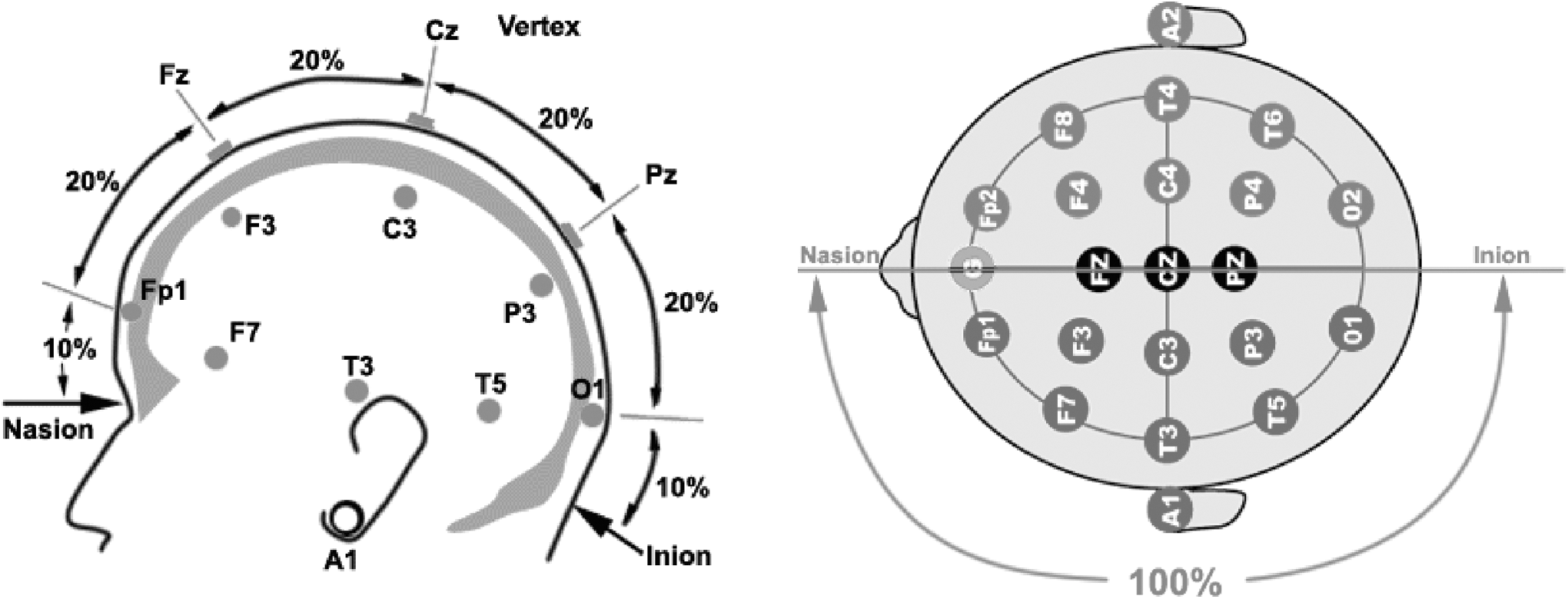
The 10/20 International system of electrode placement.

Scalp EEG recording devices use different amplifiers to compute the voltage of each EEG channel, which take as input the measurements of two electrodes and produce the corresponding EEG channel as the difference between the two inputs, after it has been amplified. The choice of input electrodes to each amplifier is known as montage and in that case, the nodes in each EEG graph represent a pair of electrodes. An EEG can be monitored with the following types of montage (Aurlien et al., 2004; Lagerlunda, 2000):

• Sequential (or Bipolar) montage: Each channel (i.e., waveform) represents the difference between two adjacent electrodes. The entire montage consists of a series of these channels, where pairs of neighboring electrodes are subtracted from one another. Usually, the pairs are taken in straight lines from the front to the back of the head. For example, the channel “Fp1-F3” represents the difference in voltage between the Fp1 electrode and the F3 electrode. The next channel in the montage, “F3-C3,” represents the voltage difference between F3 and C3 and so on, through the entire array of electrodes.

• Referential montage: Each channel represents the difference between a certain electrode and a designated reference electrode. It is also called common reference montage, since the reference electrode is common to all amplifiers. There is no standard position for this reference; it is, however, at a different position than the “recording” electrodes. Midline positions are often used because they do not amplify the signal in one hemisphere versus the other. Another popular reference is “linked ears,” which is a physical or mathematical average of electrodes attached to both earlobes or both mastoids.

• Average reference montage: The outputs of all of the amplifiers are summed and averaged, and this averaged signal is used as the common reference for each channel.

• Laplacian montage: Each channel represents the difference between an electrode and a weighted average of the surrounding electrodes (Nunez and Pilgreen, 1991).

Figure 6 summarizes the general procedure of EEG data processing. As already mentioned, the electrodes that are placed on the scalp measure and record the electrical activity of the brain and these recordings appear as signals, as shown in the second step of Figure 6. To convert the signals into graph data sets, pairwise correlations between all pairs of time series are calculated using several connectivity measures (Pereda et al., 2005), some of which are described next. Examples of using these measures in EEG studies are presented in Christodoulakis and colleagues (2015).

• Cross-correlation: Given two time series x(t) and y(t) with t ∈ {1…n}, the normalized cross-correlation function between x and y as a function of lag τ, is given by \documentclass{aastex}\usepackage{amsbsy}\usepackage{amsfonts}\usepackage{amssymb}\usepackage{bm}\usepackage{mathrsfs}\usepackage{pifont}\usepackage{stmaryrd}\usepackage{textcomp}\usepackage{portland, xspace}\usepackage{amsmath, amsxtra}\usepackage{upgreek}\pagestyle{empty}\DeclareMathSizes{10}{9}{7}{6}\begin{document}$$ { C_ { xy } } \left( { \rm { \tau } } \right) = \frac { 1 } { { n - \tau } } \mathop \sum \limits_ { t = 1 } ^ { n - \tau } \left( { \frac { x \left( t \right) } { { \sigma _x } } } \right) \left( { { \frac { y \left( { t + \tau } \right) } { { \sigma _y } } } } \right)$$ \end{document} , where σ_x and σ_y are the standard deviations of x and y, respectively. C_xy is computed for a range of values of lag τ, which depends on the sampling frequency. Note that when the mean value of both signals is not subtracted beforehand, the normalized cross-variance function should instead be as follows,: \documentclass{aastex}\usepackage{amsbsy}\usepackage{amsfonts}\usepackage{amssymb}\usepackage{bm}\usepackage{mathrsfs}\usepackage{pifont}\usepackage{stmaryrd}\usepackage{textcomp}\usepackage{portland, xspace}\usepackage{amsmath, amsxtra}\usepackage{upgreek}\pagestyle{empty}\DeclareMathSizes{10}{9}{7}{6}\begin{document}$$\mathop \sum \limits_ { t = 1 } ^ { n - \tau } \left( { \frac { x \left( t \right) - \overline x } { { \sigma _x } } } \right) \left( { { \frac { y \left( { t + \tau } \right) - \overline y } { { \sigma _y } } } } \right)$$ \end{document} . C_xy takes values between [−1,1], with 1 indicating the largest positive correlation, −1 the largest negative correlation, and 0 no correlation. For the purposes of constructing the graphs and obtaining graph theoretical measures, the absolute value of the cross-correlation is computed and the correlation between the two signals can be computed as max_τ|C_xy |, over the desired range of τ (Pereda et al., 2005).

• Corrected cross-correlation: Cross-correlation often takes its maximum at zero lag in the case of scalp EEG measurements. Consistent zero-lag correlations could be due to volume conduction effects: this is because currents from underlying sources are conducted instantaneously through the head volume to EEG sensors (assuming that scalp potentials have no delays compared to their underlying sources [quasi-static approximation]). Thus, signals arising from a common source will be simultaneously picked up by different electrodes affecting a spurious zero-lag correlation between the two electrode signals. It should be noted, although, that zero-lag correlations could also be due to a third common source or even true direct physiological interactions. In principle, true direct interactions between any two physiological sources will typically incur a nonzero delay due to transmission speed, provided that the sampling frequency is high enough to capture such delays. However, consistent nonzero lag correlations are unlikely to be due to the effects of common sources. To measure true interactions not occurring at zero lag, we calculate the odd part of cross-correlation, which is a measure of its asymmetry, as defined in Nevado et al. (2012) by subtracting the negative lag part of C_xy (τ) from its positive lag counterpart: \documentclass{aastex}\usepackage{amsbsy}\usepackage{amsfonts}\usepackage{amssymb}\usepackage{bm}\usepackage{mathrsfs}\usepackage{pifont}\usepackage{stmaryrd}\usepackage{textcomp}\usepackage{portland, xspace}\usepackage{amsmath, amsxtra}\usepackage{upgreek}\pagestyle{empty}\DeclareMathSizes{10}{9}{7}{6}\begin{document}$${ \widetilde C_{xy}} \left( \tau \right) = {C_{xy}} \left( \tau \right) - {C_{xy}} \left( { - \tau } \right)$$ \end{document} , for τ > 0. Note that \documentclass{aastex}\usepackage{amsbsy}\usepackage{amsfonts}\usepackage{amssymb}\usepackage{bm}\usepackage{mathrsfs}\usepackage{pifont}\usepackage{stmaryrd}\usepackage{textcomp}\usepackage{portland, xspace}\usepackage{amsmath, amsxtra}\usepackage{upgreek}\pagestyle{empty}\DeclareMathSizes{10}{9}{7}{6}\begin{document}$${ \widetilde C_{xy}}$$ \end{document} provides a lower bound estimate of the nonzero lag cross-correlations and is notably smaller than \documentclass{aastex}\usepackage{amsbsy}\usepackage{amsfonts}\usepackage{amssymb}\usepackage{bm}\usepackage{mathrsfs}\usepackage{pifont}\usepackage{stmaryrd}\usepackage{textcomp}\usepackage{portland, xspace}\usepackage{amsmath, amsxtra}\usepackage{upgreek}\pagestyle{empty}\DeclareMathSizes{10}{9}{7}{6}\begin{document}$${C_{xy}}$$ \end{document} .

• Coherence: Coherency is the equivalent of cross-correlation in the frequency domain. It measures the linear correlation between two signals x and y as a function of the frequency f. It is defined as the cross-spectral density between x and y normalized by the autospectral densities of x and y: \documentclass{aastex}\usepackage{amsbsy}\usepackage{amsfonts}\usepackage{amssymb}\usepackage{bm}\usepackage{mathrsfs}\usepackage{pifont}\usepackage{stmaryrd}\usepackage{textcomp}\usepackage{portland, xspace}\usepackage{amsmath, amsxtra}\usepackage{upgreek}\pagestyle{empty}\DeclareMathSizes{10}{9}{7}{6}\begin{document}$$ { \Gamma _ { xy } } \left( f \right) = { \frac { { S_ { xy } } \left( f \right) } { \sqrt { { S_ { xx } } \left( f \right) { S_ { yy } } \left( f \right) } } } $$ \end{document} , where S_xy is the cross-spectral density and S_xx and S_yy are the autospectral densities of x and y, respectively (Pereda et al., 2005). Coherency is a complex number, as the cross-spectral density is complex, whereas the autospectral density function is real. Therefore, in many cases, coherence (or the squared coherence), which is defined as the magnitude of coherency (or its square), is employed as a measure of correlation in the frequency domain, that is \documentclass{aastex}\usepackage{amsbsy}\usepackage{amsfonts}\usepackage{amssymb}\usepackage{bm}\usepackage{mathrsfs}\usepackage{pifont}\usepackage{stmaryrd}\usepackage{textcomp}\usepackage{portland, xspace}\usepackage{amsmath, amsxtra}\usepackage{upgreek}\pagestyle{empty}\DeclareMathSizes{10}{9}{7}{6}\begin{document}$${\kappa_{xy}} \left(f\right) = \frac {{\left\vert { \langle{S_{xy}} \left( f \right) \rangle} \right\vert }}{\sqrt {| \langle{S_{xx}}(f) \rangle | | \langle {S_{yy}} (f) \rangle |}}$$ \end{document} . For finite data sets, coherency is estimated by using standard power spectral density estimation methods (such as the Welch method), by dividing the EEG signals into segments of equal length and averaging the individual spectral estimates. In the above equation, <.> denotes the average over all segments (Pereda et al., 2005). The value of κ_xy (f) ranges between 0 and 1, with 1 indicating perfect linear correlation and 0 no correlation between x and y at frequency f.

• Imaginary coherence: Nolte and colleagues (2004) observed that the imaginary part of coherency is insensitive to volume conduction, while the real part is strongly affected. This is due to the fact that signals arising from the same electrical source in the brain, under the quasistatic approximation, will be volume conducted to any two recording locations with no time delay, thus influencing only the real part of the cross-spectrum. Hence, imaginary coherence is defined as the imaginary part of coherency: \documentclass{aastex}\usepackage{amsbsy}\usepackage{amsfonts}\usepackage{amssymb}\usepackage{bm}\usepackage{mathrsfs}\usepackage{pifont}\usepackage{stmaryrd}\usepackage{textcomp}\usepackage{portland, xspace}\usepackage{amsmath, amsxtra}\usepackage{upgreek}\pagestyle{empty}\DeclareMathSizes{10}{9}{7}{6}\begin{document}$${ \rm{I}}{{ \rm{C}}_{xy}} \left( f \right) = { \rm{Imag}} \left( {{ \Gamma _{xy}} \left( f \right) } \right)$$ \end{document} . As in the case of coherence, the maximum absolute value in each frequency band quantifies the correlation between the two signals in that band.

• Phase lag index (PLI): It is defined as a measure of asymmetry of the phase difference distribution between two signals (Stam et al., 2011). The instantaneous phases are obtained by first band-pass filtering the signals in the frequency bands of interest and then using the Hilbert transform to obtain the phase of the analytic signal. Phase differences (Δφ) between a given pair of channels were wrapped in the interval, π ≤ Δφ ≤ π: \documentclass{aastex}\usepackage{amsbsy}\usepackage{amsfonts}\usepackage{amssymb}\usepackage{bm}\usepackage{mathrsfs}\usepackage{pifont}\usepackage{stmaryrd}\usepackage{textcomp}\usepackage{portland, xspace}\usepackage{amsmath, amsxtra}\usepackage{upgreek}\pagestyle{empty}\DeclareMathSizes{10}{9}{7}{6}\begin{document}$$\;{ \rm{PL}}{{ \rm{I}}_{xy}} = \left\vert { \langle { \rm{sgn}} \left( { \Delta \varphi \left( \tau \right) } \right) \rangle } \right\vert$$ \end{document} , where Δφ is the instantaneous phase difference between x and y. PLI ranges between 0 and 1, with 0 indicating no correlation and 1 maximal correlation.

• Weighted phase lag index (WPLI): Vinck and colleagues (2011) argued that PLI's sensitivity to noise and volume conduction is hindered by the discontinuity of the measure, which is caused by small perturbations turning phase lags into leads and vice versa. 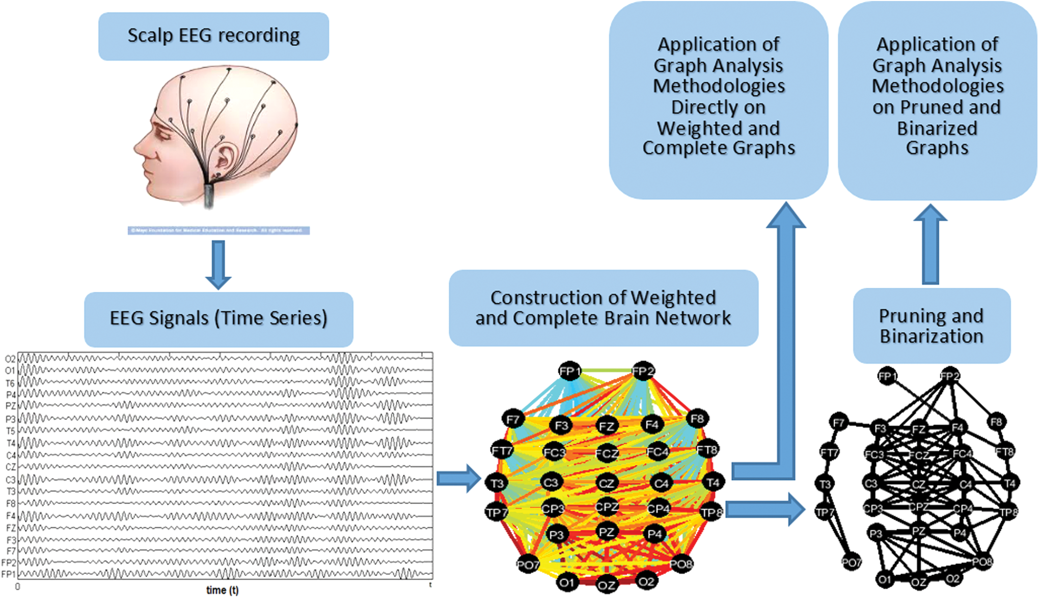To overcome this problem, they defined the WPLI, which modifies PLI by weighting the contribution of observed phase leads and lags by the magnitude of the imaginary component of the cross-spectrum as follows: \documentclass{aastex}\usepackage{amsbsy}\usepackage{amsfonts}\usepackage{amssymb}\usepackage{bm}\usepackage{mathrsfs}\usepackage{pifont}\usepackage{stmaryrd}\usepackage{textcomp}\usepackage{portland, xspace}\usepackage{amsmath, amsxtra}\usepackage{upgreek}\pagestyle{empty}\DeclareMathSizes{10}{9}{7}{6}\begin{document}$${\rm{WPLI}} = \frac {| \langle{\rm Imag} \left( {S_{xy}} (f) \right) \rangle |} {| \langle {\rm Imag}S_{xy} (f) \rangle|} = \frac {| \langle | {\rm Imag} \left(S_{xy} (f)\right)| \cdot {\rm sgn (Imag \left(S_{xy} (f)\right)\rangle}|} {{| \langle {\rm Imag} \left( {S_xy} (f) \right) \rangle} |}$$ \end{document} . Similar to PLI, WPLI ranges between 0 and 1, with 0 indicating no correlation and 1 indicating maximal correlation.

FIG. 6.

General scheme of EEG data processing. Color images available online at www.liebertpub.com/brain

After the network construction, there are two options: either apply a thresholding scheme to binarize and prune the graphs, for the purpose of processing the binarized data with graph analysis methodologies, or apply graph analysis techniques directly on weighted and fully connected graphs. The majority of the proposed methods follow the first option as binary networks are simpler and easier to study. However, some algorithms for studying weighted EEG networks have also been proposed recently (Iakovidou et al., 2013a, 2015).

The most common data structures that are used to make EEG network computer readable are adjacency matrices and adjacency lists. The following section provides a short mathematical description of these data structures:

Data Structures

The two main data structures that are used to represent and store EEG graph data are described below:

The adjacency matrix, also known as connectivity matrix, of an undirected, unweighted, and labeled graph G = (V, E) consists of an nxn matrix A = a_ij or \documentclass{aastex}\usepackage{amsbsy}\usepackage{amsfonts}\usepackage{amssymb}\usepackage{bm}\usepackage{mathrsfs}\usepackage{pifont}\usepackage{stmaryrd}\usepackage{textcomp}\usepackage{portland, xspace}\usepackage{amsmath, amsxtra}\usepackage{upgreek}\pagestyle{empty}\DeclareMathSizes{10}{9}{7}{6}\begin{document}$$A = \left( { \begin{matrix} {{a_{11}}} & \ldots & {{a_{1n}}} \\ \vdots & \ddots & \vdots \\ {{a_{n1}}} & \ldots & {{a_{nn}}} \\ \end{matrix} } \right)$$ \end{document} , where n is the total number of nodes and a_ij = 1 if (i, j) ∈ V, which practically means that nodes a_i and a_j are connected and a_ij = 0 otherwise. As mentioned before, EEG graphs are weighted and fully connected, so in that case, a_ij = w_ij and a_ii = 0. The zeros along the diagonals imply that a node is not connected to itself. Generally, the adjacency matrices of undirected graphs are symmetric because a_ij = a_ji and they require a memory space of Θ(|V| ²), which is best suited for dense graphs. The graph density shows how sparse or dense a graph is according to the number of connections per node set and it is defined as \documentclass{aastex}\usepackage{amsbsy}\usepackage{amsfonts}\usepackage{amssymb}\usepackage{bm}\usepackage{mathrsfs}\usepackage{pifont}\usepackage{stmaryrd}\usepackage{textcomp}\usepackage{portland, xspace}\usepackage{amsmath, amsxtra}\usepackage{upgreek}\pagestyle{empty}\DeclareMathSizes{10}{9}{7}{6}\begin{document}$$D = { \frac { 2 \left\vert E \right\vert } { \left\vert V \right\vert \left( { \left\vert V \right\vert - 1 } \right) } } $$ \end{document} , for undirected graphs. For all-against-all symmetric matrices, only the upper or the lower triangular part of the matrix is necessary and requires Θ(|V|) amount of memory to be allocated. Figure 7 depicts an example of a weighted, symmetric, and square adjacency matrix of a brain network such that depicted in Figure 1a. In case of fully connected graphs where all nodes are connected with each other, adjacency matrices are highly suggested.

FIG. 7.

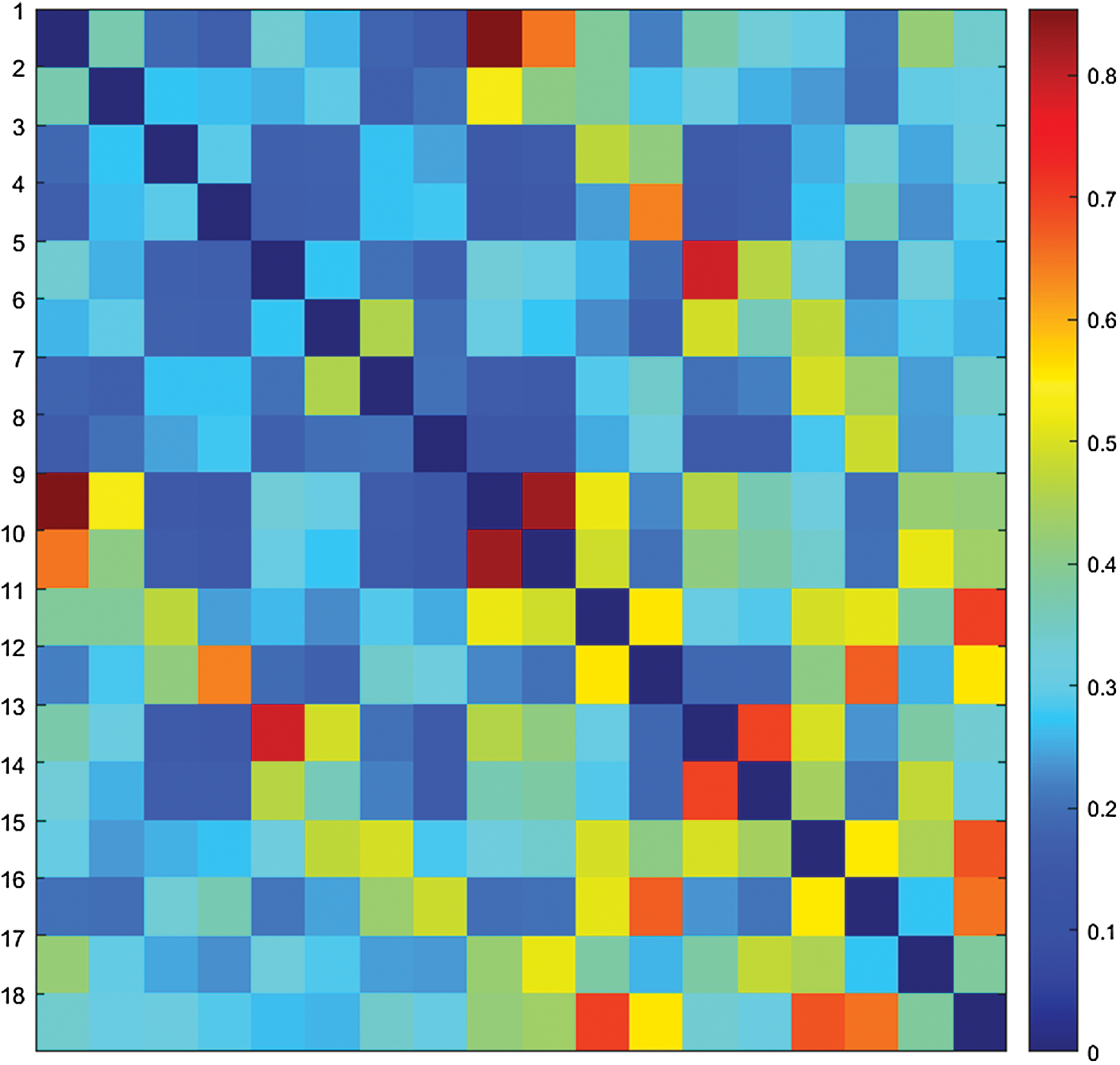
Representation of the weighted, symmetric, and square adjacency matrix of a brain network with 18 nodes. Color images available online at www.liebertpub.com/brain

To reduce memory allocation by half for large-scale data, a symmetric 2D matrix A can be stored as a 1D matrix B, where \documentclass{aastex}\usepackage{amsbsy}\usepackage{amsfonts}\usepackage{amssymb}\usepackage{bm}\usepackage{mathrsfs}\usepackage{pifont}\usepackage{stmaryrd}\usepackage{textcomp}\usepackage{portland, xspace}\usepackage{amsmath, amsxtra}\usepackage{upgreek}\pagestyle{empty}\DeclareMathSizes{10}{9}{7}{6}\begin{document}$$A \left[ { i , j } \right] = B \left[ { \frac { { i \left( { i - 1 } \right) } } { 2 } + j } \right]$$ \end{document} if the first element is a ₁₁ like, for example, in Matlab platform, or \documentclass{aastex}\usepackage{amsbsy}\usepackage{amsfonts}\usepackage{amssymb}\usepackage{bm}\usepackage{mathrsfs}\usepackage{pifont}\usepackage{stmaryrd}\usepackage{textcomp}\usepackage{portland, xspace}\usepackage{amsmath, amsxtra}\usepackage{upgreek}\pagestyle{empty}\DeclareMathSizes{10}{9}{7}{6}\begin{document}$$A \left[ { i , j } \right] = B \left[ { \frac { { i \left( { i + 1 } \right) } } { 2 } + j } \right]$$ \end{document} i if the first element is a ₀₀ like in the majority of programming languages. In both cases, matrix B hosts the lower part of matrix A. If, for example, A is a 3 × 3 matrix starting from element a ₁₁, \documentclass{aastex}\usepackage{amsbsy}\usepackage{amsfonts}\usepackage{amssymb}\usepackage{bm}\usepackage{mathrsfs}\usepackage{pifont}\usepackage{stmaryrd}\usepackage{textcomp}\usepackage{portland, xspace}\usepackage{amsmath, amsxtra}\usepackage{upgreek}\pagestyle{empty}\DeclareMathSizes{10}{9}{7}{6}\begin{document}$$A = \left( { \begin{matrix}{{a_{11}}} & {{a_{12}}} & {{a_{13}}} \\ {{a_{21}}} & {{a_{22}}} & {{a_{23}}} \\ {{a_{31}}} & {{a_{32}}} & {{a_{33}}} \\ \end{matrix} } \right)$$ \end{document} , then matrix B is defined as B = {a ₁₁, a ₂₁, a ₂₂, a ₃₁ , a ₃₂ , a ₃₃}. The 1D array will be of size \documentclass{aastex}\usepackage{amsbsy}\usepackage{amsfonts}\usepackage{amssymb}\usepackage{bm}\usepackage{mathrsfs}\usepackage{pifont}\usepackage{stmaryrd}\usepackage{textcomp}\usepackage{portland, xspace}\usepackage{amsmath, amsxtra}\usepackage{upgreek}\pagestyle{empty}\DeclareMathSizes{10}{9}{7}{6}\begin{document}$$ \frac { { n \left( { n + 1 } \right) } } { 2 } $$ \end{document} , including the diagonal.

On the contrary, sparse graphs, for example, pruned EEG graphs, are better represented by an adjacency list. Given a graph G = (V, E), its adjacency list consists of an array Adj of |E| elements where for each e∈E, Adj(0, e) = i∈V. Adjacency lists require a memory space of Θ(|V|+|E|).

Network Properties

Exploring different network properties can provide valuable insight into the internal function of brain networks and provide a better understanding of the human brain. In the following, we give a short description of the main properties that are commonly analyzed in networks, including brain networks as well.

In graph theory, an isomorphism of graphs G and H is a bijection between the vertex sets of G and H, f: V(G) → V(H), such that any two vertices u and v of G are adjacent in G if and only if f(u) and f(v) are adjacent in H. An example of isomorphic graphs is depicted in Figure 8. In case of EEG graphs, there is no question of isomorphism, because as mentioned above, each node takes its name by the specific and unchangeable positions that the electrodes have on the scalp.

FIG. 8.

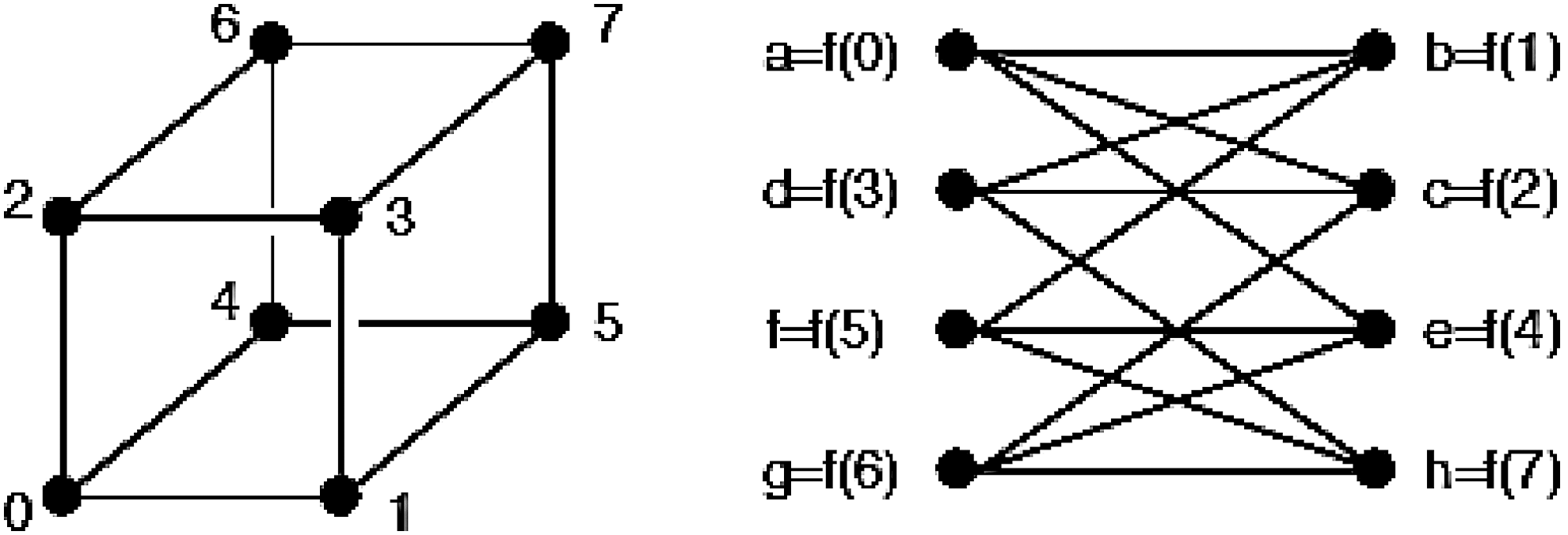
Example of isomorphism between two simple graphs.

A walk is a pass through a specific sequence of nodes (v ₁, v ₂, …, v_L ) such that (v ₁, v ₂), (v ₂, v ₃), …, (v_L − ₁, v_L ) ⊆ E. In a walk, it is possible for a node or an edge to appear more than once. If an edge does not appear two or more times, the walk is called a trail, and if a node does not appear two or more times, the walk is called a path. A cycle is a walk (v ₁, v ₂, …, v_L ) where v ₁ = v_L with no other nodes repeated and L > 3, such that the last node is the same as the first one. A graph is called cyclic if it contains a cycle and in any other case, it is called acyclic. An undirected graph is called connected if there is a path from any node to any other node in the graph.

The shortest (or geodesic) path length, d_i,j , between a pair of nodes, i and j, is the minimum number of edges that has to be traversed to get from node i to j. Then, the characteristic (or average) path length is defined as the average shortest path length over all pairs of nodes in the network. This measure also provides an indication of how well integrated the graph is and it is calculated as \documentclass{aastex}\usepackage{amsbsy}\usepackage{amsfonts}\usepackage{amssymb}\usepackage{bm}\usepackage{mathrsfs}\usepackage{pifont}\usepackage{stmaryrd}\usepackage{textcomp}\usepackage{portland, xspace}\usepackage{amsmath, amsxtra}\usepackage{upgreek}\pagestyle{empty}\DeclareMathSizes{10}{9}{7}{6}\begin{document}$$L = \frac { 1 } { { n \left( { n - 1 } \right) } } \mathop \sum \limits_ { i \in N } \mathop \sum \limits_ { j \in N , i \ne j } { d_ { i , j } } $$ \end{document} , where N denotes the set of all nodes in the graph and n is the total number of such nodes. The most common algorithms for calculating the shortest paths are Dijkstra's greedy algorithm (Dijkstra, 1959) and Floyd's dynamic algorithm (Floyd, 1962). Dijkstra's algorithm has running time complexity O(N ²), where N is the number of vertices and returns the shortest path between a source vertex i and all other vertices in the network. Floyd's algorithm has running time complexity O(N ³) and requires an all-against-all matrix that contains the distances of every node in the network to every other node in the network.

The efficiency of a path between two vertices (local efficiency) (De Vico Fallani et al., 2010) is defined as the inverse of the shortest distance between the vertices. When such a path does not exist, the efficiency is zero. Global efficiency (Latora and Marchiori, 2001) is the average efficiency over all pairs of nodes and is a measure of how efficiently the information is exchanged across the whole network. The efficiency of a network can be used to quantify small world behavior in networks, which is described later on in the document, and it is defined as follows: \documentclass{aastex}\usepackage{amsbsy}\usepackage{amsfonts}\usepackage{amssymb}\usepackage{bm}\usepackage{mathrsfs}\usepackage{pifont}\usepackage{stmaryrd}\usepackage{textcomp}\usepackage{portland, xspace}\usepackage{amsmath, amsxtra}\usepackage{upgreek}\pagestyle{empty}\DeclareMathSizes{10}{9}{7}{6}\begin{document}$$E = \frac { 1 } { { n \left( { n - 1 } \right) } } \mathop \sum \limits_ { i \in N } \mathop \sum \limits_ { j \in N , i \ne j } ^n d_ { i , j } ^ { - 1 } $$ \end{document} .

The clustering coefficient is the measurement that shows the tendency of a graph to be divided into clusters. A cluster is a subset of vertices that contains lots of edges connecting these vertices to each other. Consequently, this measurement identifies groups of nodes that are largely connected with other nodes in the same group, but have a much smaller number of connections to nodes outside their group. Formally, the clustering coefficient (or local clustering coefficient) (Watts and Strogatz, 1998) of a node i is \documentclass{aastex}\usepackage{amsbsy}\usepackage{amsfonts}\usepackage{amssymb}\usepackage{bm}\usepackage{mathrsfs}\usepackage{pifont}\usepackage{stmaryrd}\usepackage{textcomp}\usepackage{portland, xspace}\usepackage{amsmath, amsxtra}\usepackage{upgreek}\pagestyle{empty}\DeclareMathSizes{10}{9}{7}{6}\begin{document}$$ { C_i } = { \frac { 2 { t_i } } { { k_i } \left( { { k_i } - 1 } \right) } } $$ \end{document} , where k_i is the degree of node i and t_i denotes the number of edges between neighbors of i. Then the global clustering coefficient C of the network is defined as the mean clustering coefficient among all nodes: \documentclass{aastex}\usepackage{amsbsy}\usepackage{amsfonts}\usepackage{amssymb}\usepackage{bm}\usepackage{mathrsfs}\usepackage{pifont}\usepackage{stmaryrd}\usepackage{textcomp}\usepackage{portland, xspace}\usepackage{amsmath, amsxtra}\usepackage{upgreek}\pagestyle{empty}\DeclareMathSizes{10}{9}{7}{6}\begin{document}$$C = \frac { 1 } { n } \mathop \sum \limits_ { i \in N } { C_i } $$ \end{document} .

Network small-worldness

A network is called small world when it is highly clustered (large C), while at the same time it has a small characteristic path length (L) (Watts and Strogatz, 1998). The network small-worldness (Humphries and Gurney, 2008) measures how close to being small-world a network is. Formally, it is defined as \documentclass{aastex}\usepackage{amsbsy}\usepackage{amsfonts}\usepackage{amssymb}\usepackage{bm}\usepackage{mathrsfs}\usepackage{pifont}\usepackage{stmaryrd}\usepackage{textcomp}\usepackage{portland, xspace}\usepackage{amsmath, amsxtra}\usepackage{upgreek}\pagestyle{empty}\DeclareMathSizes{10}{9}{7}{6}\begin{document}$$S = { \frac { C / { C_ { { \rm { rand } } } } } { L / { L_ { { \rm { rand } } } } } } $$ \end{document} , where C and L are the clustering coefficient and the characteristic path length of the network, while C _rand and L _rand are those of a random network of the same size, respectively. Values S ≫ 1 indicate that the network is small-world. Some studies provide evidence for the existence of functional networks in the human brain, exhibiting small-world attributes (Bassett et al., 2006; Sporns and Honey, 2006). All the aforementioned properties can be computed for both binary and weighted EEG networks (Rubinov and Sporns, 2010).

Network motifs have been identified as patterns of interconnections appearing in significantly higher number than in randomized networks, in a given ensemble of anatomical or functional connectivity graphs (Milo et al., 2002). Given a graph G, a motif is a small connected subgraph G′ of graph G. In many studies, detecting and enumerating motifs in brain networks require a predetermined motif repertoire and the proposed approaches can operate only with predefined number of motifs of small size (consisting of few nodes) (De Vico Fallani et al, 2007, 2008b; Sporns and Kotter, 2004). However, new methods have been proposed lately that detect intelligently, size-free network motifs instead of exhaustively enumerating the number of occurrences of each subnetwork of a given size k (Iakovidou et al., 2013a,b).

A clique in an undirected graph G is a subgraph G′, which is complete. The size of a clique comes from the number of vertices it contains. A maximal clique is a clique that cannot be extended by including one additional adjacent vertex, that is, a clique that does not exist exclusively within the vertex set of a larger clique. A maximum clique is a clique of the largest possible size in a given graph. The clique problem refers to the problem of finding the largest clique in any graph G. This problem is NP-complete (Garey and Johnson, 1979) and as such, many consider that it is unlikely that an efficient algorithm for finding the largest clique of a graph exists. A very famous method to find maximal cliques in a graph is the so-called Bron-Kerbosch algorithm (Bron and Kerbosch, 1973). Detection and analysis of these structures have many practical applications, for example, use of cliques to extend the concept of motif (Wang et al., 2012) and also to measure the cognitive activity with applications in the clinical diagnosis of cognitive impairments (Vijayalakshmi et al., 2015b).

In graph theory, a tree is an undirected graph in which any two vertices are connected by exactly one path; in other words, tree is called any connected graph that does not contain cycles. A spanning tree of a graph G is a subgraph G′ that connects all the vertices together and contains no cycles. A minimum spanning tree (MST) is a spanning tree of a connected, undirected graph that connects all the vertices together with the minimal total weighting for its edges. MSTs are gaining ground lately in the study of EEG brain networks since they can be directly applied to weighted EEG graphs and practically produce thresholded subgraphs that can be studied more easily and produce useful results, for example, to detect network changes in patients, but they also help to increase comparability between studies (Tewarie et al., 2014, 2015). Kruskal's (Kruskal, 1956) and Prim's (Prim, 1957) algorithms are the most popular ones to detect an MST in connected, weighted, and undirected graphs.

Network Topology and Measures

This section shows how nodes can be ranked or sorted according to their properties, depending on the question asked. In brain networks, it is important, for example, to detect central nodes or intermediate nodes that affect the topology of the network, in order, for example, to study brain diseases such as Alzheimer (Engels et al., 2015) and epilepsy (Christodoulakis et al., 2012).

Scale-free networks occur in many areas of science and engineering, including, for example, the topology of the World Wide Web (www). In www, the nodes are individual web pages and represent publications, while the links are hyperlinks, or peer-reviewed scientific literature and denote citations. Recently, it has been proved that many brain networks present scale-free properties as well (Eguiluz et al., 2005; Lee et al., 2010; Stam and de Bruin, 2004; Van de Ville et al., 2010). A scale-free network is a connected graph with the property that the number of links k originating from a given node exhibits a power law distribution \documentclass{aastex}\usepackage{amsbsy}\usepackage{amsfonts}\usepackage{amssymb}\usepackage{bm}\usepackage{mathrsfs}\usepackage{pifont}\usepackage{stmaryrd}\usepackage{textcomp}\usepackage{portland, xspace}\usepackage{amsmath, amsxtra}\usepackage{upgreek}\pagestyle{empty}\DeclareMathSizes{10}{9}{7}{6}\begin{document}$$P \left( k \right) \sim{k^{ - \gamma }}$$ \end{document} , where γ denotes the degree exponent. A scale-free network can be constructed by progressively adding nodes to an existing network and introducing links to existing nodes with preferential attachment so that the probability of linking to a given node i is proportional to the number of existing links k_i that the node has. Thus, the connectivity of one node i to any other node j should follow the rule \documentclass{aastex}\usepackage{amsbsy}\usepackage{amsfonts}\usepackage{amssymb}\usepackage{bm}\usepackage{mathrsfs}\usepackage{pifont}\usepackage{stmaryrd}\usepackage{textcomp}\usepackage{portland, xspace}\usepackage{amsmath, amsxtra}\usepackage{upgreek}\pagestyle{empty}\DeclareMathSizes{10}{9}{7}{6}\begin{document}$$P \left( { { \rm { links \_to \_node } } \_i } \right) \sim { \frac { { k_i } } { \sum \nolimits_j { k_j } } } $$ \end{document} .

Degree centrality

Degree centrality shows that an important node is involved in a large number of interactions. For a node i, the degree centrality is calculated as C_d (i) = k(i), as already described in Basic Graph Theory Definitions and Terms section. Nodes with very high degree centrality are called hubs and represent important brain regions that often interact with many other regions and also facilitate functional integration, and generally play a key role in network resilience to insult (Rubinov and Sporns, 2010; van den Heuvel and Sporns, 2013). Scale-free networks tend to contain hubs and the removal of such central nodes has great impact on the topology of the network (van Straaten and Stam, 2013). Another measure that is valid for weighted graphs only is the node strength s(i), which is defined as the sum of weights of the links connected to the node i (Barrat et al., 2004).

Many measures of centrality are based on the idea that central nodes participate in many short paths within a network and consequently act as important controls of information flow (Freeman, 1979). For instance, closeness centrality indicates important nodes that can communicate quickly with other nodes of the network, or in other words, the efficiency of a node in spreading information to all other nodes of the network. Let G = (V, E) be an undirected graph. Then, the closeness centrality of a node i is defined as \documentclass{aastex}\usepackage{amsbsy}\usepackage{amsfonts}\usepackage{amssymb}\usepackage{bm}\usepackage{mathrsfs}\usepackage{pifont}\usepackage{stmaryrd}\usepackage{textcomp}\usepackage{portland, xspace}\usepackage{amsmath, amsxtra}\usepackage{upgreek}\pagestyle{empty}\DeclareMathSizes{10}{9}{7}{6}\begin{document}$$ { C_ { { \rm { clo } } \left( i \right) } } = \frac { 1 } { { \mathop \sum \nolimits_ { t \in V } ^ { \left\vert V \right\vert } { \rm { dist } } \left( { i , j } \right) } } $$ \end{document} , where dist(i, j) denotes the distance or else, the shortest path p between the nodes i and j.

A related and often more sensitive measure is betweenness centrality (Freeman, 1979) C_b (i) of a node i, which measures how many geodesic paths between any pair of nodes pass through i. It is a measure of the importance of a node, because the higher the betweenness centrality, the shortest paths will need to be rerouted in case of damage to that node. Formally, \documentclass{aastex}\usepackage{amsbsy}\usepackage{amsfonts}\usepackage{amssymb}\usepackage{bm}\usepackage{mathrsfs}\usepackage{pifont}\usepackage{stmaryrd}\usepackage{textcomp}\usepackage{portland, xspace}\usepackage{amsmath, amsxtra}\usepackage{upgreek}\pagestyle{empty}\DeclareMathSizes{10}{9}{7}{6}\begin{document}$$ { C_b } \left( i \right) = \frac { 1 } { { \left( { n - 1 } \right) \left( { n - 2 } \right) } } \mathop \sum \limits_ { j , k \in N , j \ne k } { \frac { { n_ { j , k } } \left( i \right) } { { n_ { j , k } } } } $$ \end{document} , where n_j,k is the number of shortest paths between j and k and n_j,k (i) is the number of such paths that pass through node i. Then, betweenness centralization (de Nooy et al., 2011) is a measure that summarizes the variation in betweenness centrality in the network. It is defined as the ratio of the variation in betweenness centrality among all nodes in the network to the maximum such variation in any network of the same size. The calculation of betweenness centrality has been made significantly more efficient with the recent development of faster algorithms (Brandes, 2001; Kintali, 2008).

Eigenvector centrality

Eigenvector centrality generally ranks higher the nodes that are connected to important neighbors (Batool and Niazi, 2014). Consequently, a node has high value of eigenvector centrality either if it is connected to many other nodes or if it is connected to others that themselves have high eigenvector centrality. Let G = (V, E) be an undirected graph and A the adjacency matrix of network G. The eigenvector centrality is the eigenvector C _eiv of the largest eigenvalue λ _max in absolute value such that λC _eiv = AC _eiv. Formally, if A is the adjacency matrix of a network G with V(G) = v _1, …, v_n and ρ(A) = max|λ|, then the eigenvector centrality C _eiv(v_i ) of the node v_i is given by the ith coordinate x_i of a normalized eigenvector that satisfies the condition Ax = ρ(A)x.

Eccentricity centrality

Eccentricity centrality is the measure that shows how easily accessible a node is from other nodes. Let G = (V, E) be an undirected graph. The eccentricity centrality is calculated as \documentclass{aastex}\usepackage{amsbsy}\usepackage{amsfonts}\usepackage{amssymb}\usepackage{bm}\usepackage{mathrsfs}\usepackage{pifont}\usepackage{stmaryrd}\usepackage{textcomp}\usepackage{portland, xspace}\usepackage{amsmath, amsxtra}\usepackage{upgreek}\pagestyle{empty}\DeclareMathSizes{10}{9}{7}{6}\begin{document}$$ { C_ { ecc } } = \frac { 1 } { { { \rm { max } } \left( { { \rm { dist } } \left( { i , j } \right) } \right) } } $$ \end{document} , where dist(i, j) is the shortest path between nodes i and j. The eccentricity C _ecc of a vertex V is the greatest distance between v and any other vertex (Batool and Niazi, 2014).

Subgraph centrality

Subgraph centrality (Estrada and Rodriguez-Velazquez, 2005) is a new centrality measure that characterizes the participation of each node in all subgraphs in a network. Smaller subgraphs are given more weight than larger ones, which makes this measure appropriate for characterizing network motifs. The subgraph centrality can be obtained mathematically from the spectra of the adjacency matrix of the network. This measure is better able to discriminate the nodes of a network than alternate measures such as degree, closeness, betweenness, and eigenvector centralities. Let G = (V, E) be an undirected graph and A the adjacency matrix of network G. The number of closed walks of length k starting and ending on node i in the network is given by the local spectral moments, which are simply defined as the ith diagonal entry of the kth power of the adjacency matrix A. Consequently, the subgraph centrality of a node i is calculated as \documentclass{aastex}\usepackage{amsbsy}\usepackage{amsfonts}\usepackage{amssymb}\usepackage{bm}\usepackage{mathrsfs}\usepackage{pifont}\usepackage{stmaryrd}\usepackage{textcomp}\usepackage{portland, xspace}\usepackage{amsmath, amsxtra}\usepackage{upgreek}\pagestyle{empty}\DeclareMathSizes{10}{9}{7}{6}\begin{document}$$ { C_ { sg } } \left( i \right) = \mathop \sum \limits_ { k = 0 } ^ \infty { \frac { { { \left( { { A^k } } \right) } _ { ii } } } { k! } } $$ \end{document} .

Matching index

Matching index is the measure that shows how similar two nodes are within the network, by computing the amount of overlap in the connection patterns of any two nodes in the network. Two vertices that are functionally similar do not always have to be connected. The matching index M_ij measures the similarity of two nodes and is based on the number of common neighbors shared by nodes i and j. It is applied to binary networks only and it is calculated as \documentclass{aastex}\usepackage{amsbsy}\usepackage{amsfonts}\usepackage{amssymb}\usepackage{bm}\usepackage{mathrsfs}\usepackage{pifont}\usepackage{stmaryrd}\usepackage{textcomp}\usepackage{portland, xspace}\usepackage{amsmath, amsxtra}\usepackage{upgreek}\pagestyle{empty}\DeclareMathSizes{10}{9}{7}{6}\begin{document}$$M = { \frac { \sum { \rm { common \_neighbors } } } { \sum { \rm { total \_number \_of \_neighbors } } } } $$ \end{document} .

It is very often the case that studies of a particular brain network involve the analysis of functional brain network topology and the comparison of several centrality measures (Fraschini et al., 2015). Further measurements and their applications to the study of brain connectivity in general can be found in Rubinov and Sporns (2010). Also, the majority of these measures, for both binary and weighted networks, have been implemented in the brain connectivity Matlab toolbox, which is available online (www.brain-connectivity-toolbox.net). Finally, tools that have implemented functionality for exploring the different types of centralities in brain networks and complex networks in general are presented in Baur and colleagues (2002), de Nooy and colleagues (2011), and De Vico Fallani and colleagues (2014).

Discussion and Conclusions

The first very important conclusion is that graph theory and theory of networks constitute a very useful tool for the study of EEG brain networks and generally for large-scale brain networks as well. The reason for this is that, these theories provide powerful realistic ways to model and describe complex brain networks, but also a large and continuously increasing number of robust measures to study topological and dynamical properties of these networks. As already mentioned, EEGs are spatiotemporal data and graph theory allows us to explore both the spatial and temporal nature of these data and helps us to better understand the correlations between network structure and the processes that are taking place in these networks through time.

However, there are some methodological issues that have to be considered during the study of EEG signals as graphs. For example, it is well established that both volume conduction (Blum and Rutkove, 2007) and the choice of recording reference (montage) affect the connectivity measures obtained from scalp EEGs, in the time and frequency domains (Christodoulakis et al., 2015). Although a number of measures have been proposed aiming to reduce this influence (Guevara et al., 2005; Nunez et al., 1999; Peraza et al., 2012; Thatcher, 2012) (some of them were presented in Basic EEG Recording Properties and Construction of Brain Networks section), the optimal way to convert all EEGs, both in health and disease, into graph datasets has not been clear yet. Also, anyone who studies EEG data must know that these data are typically contaminated with artifacts (e.g., by eye movements) (Nolan et al., 2010). The effect of artifacts can be attenuated by deleting, for example, data with amplitudes over a certain value. For this reason, researchers usually apply independent component analysis (Hyvarinen and Oja, 2000) to separate EEG data into neural activity and artifact, and once identified, artifactual components can be deleted from the data.

Another point is the somewhat arbitrary threshold that has to be set sometimes to convert a weighted functional connectivity network into an unweighted (binarized) graph. The choice of the threshold remains arbitrary and studying a whole range of thresholds may raise statistical problems because of the large number of tests to be done (Stam and Reijneveld, 2007). A further problem that may occur when converting matrices of correlations to binarized graphs, depending of course from the thresholding methodology that is used, is the fact that some of the nodes may become disconnected from the network. This fact will bring difficulties in the calculation of clustering coefficients and path lengths, but the use of global and local efficiency measures might provide a solution in that case (Newman, 2003). However, if someone chooses to use the MST for pruning the graph, then no such matter will occur since the MST connects all the vertices of the graph. Another remark is that functional connectivity networks would be better to be studied as weighted graphs, to take into account the full information that is available from them, but until this time, only few methodologies are available for weighted graphs. Future studies could gain by a careful consideration of all the graph measures that are currently available and the new measures that are continually developed.

Another subject that presents high interest is the frequent subgraph mining methodologies (Jiang et al., 2013; Vijayalakshmi et al., 2015a) that rely on graph structure to discover features that better discriminate between different groups of graphs (Craddock et al., 2015; Iakovidou et al., 2013b; Thoma et al., 2010). The discovery of group-consistent connected subgraphs, which are also called motifs, can be used either to characterize a particular brain state or a brain state with respect to a reference state, and the functional role of these subgraphs can be directly deduced due to the topographic configuration of the included nodes. The majority of the existing methodologies suffer from need of enumerating all the possible subnetworks of a certain size and hence its use is feasible only in the case of moderate-sized sets of graphs and for detecting motifs of small size (Kashani et al., 2009; Schmidt et al., 2012). However, new methods that intelligently detect size-free network motifs instead of exhaustively enumerating the number of occurrences of each subnetwork of a given size k have also been proposed (Iakovidou et al., 2013a,b). All these studies have been made for binary graphs, although in the future, the full exploitation of connectivity weights (Jiang et al., 2010; Yang et al., 2012) should be considered, to avoid any arbitrariness induced by the binarization step and also enhance the quality of the obtained results.

Footnotes

Acknowledgment

The author would like to thank the State Scholarships Foundation of Greece for financing this work.

Author Disclosure Statement

No competing financial interests exist.

References

Abou-Khalil

, Misulis

. 2006. Atlas of EEG & Seizure Semiology. Amsterdam, The Netherlands: Butterworth-Heinemann, Elsevier.

Aurlien

, Gjerde

, Aarseth

, Eldoen

, Karlsen

, Skeidsvoll

, Gilhus

. 2004. EEG background activity described by a large computerized database. Clin Neurophysiol, 115:665–673.

Barrat

, Barthelemy

, Pastor-Satorras

, Vespignani

. 2004. The architecture of complex weighted networks. Proc Natl Acad Sci U S A, 101:3747–3752.

Bassett

, Meyer-Lindenberg

, Achard

, Duke

, Bullmore

. 2006. Adaptive reconfiguration of fractal small-world human brain functional networks. Proc Natl Acad Sci U S A, 103:19518–19523.

Bassett

, Wymbs

, Porter

, Mucha

, Carlson

, Grafton

. 2011. Dynamic reconfiguration of human brain networks during learning. Proc Natl Acad Sci U S A, 108:7641–7646.

Batool

, Niazi

. 2014. Towards a methodology for validation of centrality measures in complex networks. PLoS One, 9:e98379.

Baur

, Benkert

, Brandes

, Cornelsen

, Gaertler

, Kopf

, et al. Visone—Software for Visual Social Network Analysis. In Proceedings of the 9th International Symposium on Graph Drawing, vol. 2265, London, United Kingdom, 2002, p. 463.

Blum

, Rutkove

. 2007. Clinical Neurophysiology Primer. New York: Humana Press, Springer.

Brandes

. 2001. A faster algorithm for betweenness centrality. J Math Sociol, 25:163–177.

10.

Brigo

. 2011. Intermittent rhythmic delta activity patterns. Epilepsy Behav, 20:254–256.

11.

Bron

, Kerbosch

. 1973. Algorithm 457: finding all cliques of an undirected graph. Commun ACM, 16:575–577.

12.

Brunet

, Murray

, Michel

. 2011. Spatiotemporal analysis of multichannel EEG: CARTOOL. Comput Intell Neurosci, 2011:813870.

13.

Bullmore

, Sporns

. 2009. Complex brain networks: graph theoretical analysis of structural and functional systems. Nat Rev Neurosci, 10:186–198.

14.

Buzsaki

. 2007. Rhythms of the Brain. Oxford, UK: Oxford University Press.

15.

Cahn

, Polich

. 2006. Meditation states and traits: EEG, ERP, and neuroimaging studies. Psychol Bull, 132:180–211.

16.

Cardillo

, Petri

, Nicosia

, Sinatra

, Gomez-Gardenes

, Latora

. 2014. Evolutionary dynamics of time-resolved social interactions. Phys Rev E Stat Nonlin Soft Matter Phys, 90:052825.

17.

Christodoulakis

, Anastasiadou

, Papacostas

, Papathanasiou

, Mitsis

. Investigation of Network Brain Dynamics from EEG Measurements in Patients with Epilepsy Using Graph-Theoretic Approaches. In Proceedings of the 12th IEEE International Conference on Bioinformatics and Bioengineering (BIBE), Larnaca, Cyprus, 2012, p. 303.

18.

Christodoulakis

, Hadjipapas

, Papathanasiou

, Anastasiadou

, Papacostas

, Mitsis

. 2015. On the effect of volume conduction on graph theoretic measures of brain networks in epilepsy. In: Sakkalis

(ed.) Modern Electroencephalographic Assessment Techniques, vol. 91; p. 103. New York, NY: Springer.

19.

Cohen

, Havlin

. 2010. Complex Networks: Structure, Robustness and Function. Cambridge, UK: Cambridge University Press.

20.

Cormen

, Leiserson

, Rivest

, Stein

. 2009. Introduction to Algorithms, 3rd ed. Cambridge, MA: MIT Press.

21.

Craddock

, Tungaraza

, Milham

. 2015. Connectomics and new approaches for analyzing human brain functional connectivity. Gigascience, 4:13.

22.

De Nooy

, Mrvar

, Batagelj

. 2011. Exploratory Social Network Analysis with Pajek. Cambridge, UK: Cambridge University Press.

23.

De Pasquale

, Della Penna

, Sporns

, Romani

, Corbetta

. 2015. A dynamic core network and global efficiency in the resting human brain. Cereb Cortex, 25:1–19.

24.

De Vico Fallani

, Astolfi

, Cincotti

, Mattia

, Marciani

, Tocci

, et al. 2008a. Cortical network dynamics during foot movements. Neuroinformatics, 6:23–34.

25.

De Vico Fallani

, da Fontoura Costa

, Rodriguez

, Astolfi

, Vecchiato

, Toppi

, et al. 2010. A graph-theoretical approach in brain functional networks. Possible implications in EEG studies. Nonlinear Biomed Phys, 4(Suppl 1):S8.

26.

De Vico Fallani

, Richiardi

, Chavez

, Achard

. 2014. Graph analysis of functional brain networks: practical issues in translational neuroscience. Philos Trans R Soc Lond B Biol Sci, 369:20130521.

27.

De Vico Fallani

, Astolfi

, Cincotti

, Mattia

, Marciani

, Salinari

, et al. 2007. Cortical functional connectivity networks in normal and spinal cord injured patients: evaluation by graph analysis. Hum Brain Mapp, 28:1334–1346.

28.

De Vico Fallani

, Latora

, Astolfi

, Cincotti

, Mattia

, Marciani

, et al. 2008b. Persistent patterns of interconnection in time-varying cortical networks estimated from high-resolution EEG recordings in humans during a simple motor act. J Phys A Math Theor, 41:224014.

29.

Del Mondo

, Rodrguez

, Claramunt

, Bravo

, Thibaud

. 2013. Modeling consistency of spatio-temporal graphs. Data Knowl Eng, 84:59–80.

30.

Dijkstra

. 1959. A note on two problems in connection with graphs. Numer Math, 1:269–271.

31.

Dimitriadis

, Laskaris

, Tsirka

, Vourkas

, Micheloyannis

. 2012. An EEG study of brain connectivity dynamics at the resting state. Nonlinear Dynamics Psychol Life Sci, 16:5–22.

32.

Dimitriadis

, Laskaris

, Tsirka

, Vourkas

, Micheloyannis

, Fotopoulos

. 2010. Tracking brain dynamics via time-dependent network analysis. J Neurosci Methods, 193:145–155.

33.

Eguiluz

, Chialvo

, Cecchi

, Baliki

, Apkarian

. 2005. Scale-free brain functional networks. Phys Rev Lett, 94:018102.

34.

Engels

, Stam

, van der Flier

, Scheltens

, de Waal

, van Straaten

. 2015. Declining functional connectivity and changing hub locations in Alzheimer's disease: an EEG study. BMC Neurol, 15:145–152.

35.

Estrada

, Rodriguez-Velazquez

. 2005. Subgraph centrality in complex networks. Phys Rev E Stat Nonlin Soft Matter Phys, 71:e98379.

36.

Floyd

. 1962. Algorithm 97: shortest path. Commun ACM, 5:345.

37.

Fraschini

, Hillebrand

, Demuru

, Didaci

, Marcialis

. 2015. An EEG-based biometric system using eigenvector centrality in resting state brain networks. IEEE Signal Proc Lett, 22:186–195.

38.

Freeman

. 1979. Centrality in social networks conceptual clarification. Soc Netw, 1:215–239.

39.

Friston

. 1994. Functional and effective connectivity in neuroimaging: a synthesis. Hum Brain Mapp, 2:56–78.

40.

Garey

, Johnson

. 1979. Computers and Intractibility: A Guide to the Theory of NP-Completeness. New York, NY: W. H. Freeman.

41.

Gold

. 1999. Does 40-hz oscillation play a role in visual consciousness?. Conscious Cogn, 8:186–195.

42.

Greenfield

, Geyer

, Carney

. 2010. Reading EEGs: A Practical Approach. Baltimore, MD: Lippincorr Williams & Wilkins.

43.

Gribkov

, Gribkova

. 2000. Learning dynamics from non-stationary time series: analysis of electroencephalograms. Phys Rev E Stat Phys Plasmas Fluids Relat Interdiscip Topics, 61:6538–6545.

44.

Guevara

, Luis

, Velazquez

, Nenadovic

, Wennberg

, Senjanovi

, et al. 2005. Phase synchronization measurements using electroencephalographic recordings: what can we really say about neuronal synchrony?. Neuroinformatics, 3:301–314.

45.

Hughes

. 2008. Gamma, fast, and ultrafast waves of the brain: their relationships with epilepsy and behavior. Epilepsy Behav, 13:25–31.

46.

Humphries

, Gurney

. 2008. Network small-world-ness': a quantitative method for determining canonical network equivalence. PLoS One, 3:e0002051.

47.

Hyvarinen

, Oja

. 2000. Independent component analysis: algorithms and applications. Neural Netw, 13:411430.

48.

Iakovidou

, Christodoulakis

, Papathanasiou

, Papacostas

, Mitsis

. Introducing Weighted Approaches to Study Network Brain Dynamics from EEG Epilepsy Measurements: The EigenBrain Algorithm. In Proceedings of the 15th IEEE International Conference on Bioinformatics and Bioengineering (BIBE), Belgrade, Serbia, 2015, p. 1.

49.

Iakovidou

, Dimitriadis

, Laskaris

, Tsichlas

. Querying Functional Brain Connectomics to Discover Consistent Subgraph Patterns. In Proceedings of the 13th IEEE International Conference on Bioinformatics and Bioengineering (BIBE), Chania, Greece, 2013a, p. 1.

50.

Iakovidou

, Dimitriadis

, Laskaris

, Tsichlas

, Manolopoulos

. 2013b. On the discovery of group-consistent graph substructure patterns from brain networks. J Neurosci Methods, 213:204–213.

51.

Iasemidis

. 2011. Seizure prediction and its applications. Neurosurg Clin N Am, 22:489–506.

52.

Jiang

, Coenen

, Zito

. Frequent Sub-graph Mining on Edge Weighted Graphs. In Proceedings of the 12th International Conference on Data Warehousing and Knowledge Discovery, Bilbao, Spain, 2010, p. 77.

53.

Jiang

, Coenen

, Zito

. 2013. A survey of frequent subgraph mining algorithms. Knowl Eng Rev, 28:75–105.

54.

Joudaki

, Salehi

, Jalili

, Knyazeva

. 2012. EEG-based functional brain networks: does the network size matter?. PLoS One, 7:e35673.

55.

Joyce

, Laurienti

, Burdette

, Hayasaka

. 2010. A new measure of centrality for brain networks. PLoS One,, 5:e12200.

56.

Jurcak

, Tsuzuki

, Dan

. 2007. 10/20, 10/10, and 10/5 systems revisited: their validity as relative head-surface-based positioning systems. Neuroimage, 34:1600–1611.

57.

Kashani

, Ahrabian

, Elahi

, Nowzari-Dalini

, Saberi

, Asadi

, et al. 2009. Kavosh: a new algorithm for finding network motifs. BMC Bioinformatics, 10:318.

58.

Kintali

. 2008. Betweenness centrality: algorithms and lower bounds. arXiv:0809.1906 [cs.DS].

59.

Kramarenko

, Tan

. 2003. Effects of high-frequency electromagnetic fields on human EEG: a brain mapping study. Int J Neurosci, 113:1007–1019.

60.

Kruskal

. 1956. On the shortest spanning subtree of a graph and the traveling salesman problem. Proc Am Math Soc, 7:48–50.

61.

Lagerlunda

. 2000. Manipulating the magic of digital EEG: montage reformatting and filtering. Am J Electroneurodiagn Technol, 40:121–136.

62.

Latora

, Marchiori

. 2001. Efficient behavior of small-world networks. Phys Rev Lett, 87:198701.

63.

Lee

, Oh

, Kim

, Noh

, Choi

, Mashour

. 2010. Brain networks maintain a scale-free organization across consciousness, anesthesia, and recovery: evidence for adaptive reconfiguration. Anesthesiology, 113:1081–1091.

64.

Milo

, Shen-Orr

, Itzkovitz

, Kashtan

, Chklovskii

, Alon

. 2002. Network motifs: simple building blocks of complex networks. Science, 298:824–827.

65.

Nevado

, Hadjipapas

, Kinsey

, Moratti

, Barnes

, Holliday

, Green

. 2012. Estimation of functional connectivity from electromagnetic signals and the amount of empirical data required. Neurosci Lett, 513:57–61.

66.

Newman

. 2003. The structure and function of complex networks. SIAM Rev, 45:167256.

67.

Niedermeyer

. 1997. Alpha rhythms as physiological and abnormal phenomena. Int J Psychophysiol, 26:31–49.

68.

Niedermeyer

, Lopes da Silva

. 2012. Electroencephalography: Basic Principles, Clinical Applications, and Related Fields, 5th ed. Baltimore, MD: Lippincott Williams & Wilkins.

69.

Nolan

, Whelan

, Reilly

. 2010. FASTER: fully automated statistical thresholding for EEG artifact rejection. J Neurosci Methods, 192:152162.

70.

Nolte

, Bai

, Wheaton

, Mari

, Vorbach

, Hallett

. 2004. Identifying true brain interaction from EEG data using the imaginary part of coherency. Clin Neurophysiol, 115:2292–2307.

71.

Nunez

, Pilgreen

. 1991. The spline-laplacian in clinical neurophysiology: a method to improve EEG spatial resolution. Clin Neurophysiol, 8:397–413.

72.

Nunez

, Silberstein

, Shi

, Carpenter

, Srinivasan

, Tucker

, et al. 1999. EEG coherency II: experimental comparisons of multiple measures. Clin Neurophysiol, 110:469–483.

73.

Nunez

, Srinivasan

. 2006a. Electric Fields of the Brain: The Neurophysics of EEG. Oxford, UK: Oxford University Press.

74.

Nunez

, Srinivasan

. 2006b. A theoretical basis for standing and traveling brain waves measured with human EEG with implications for an integrated consciousness. Clin Neurophysiol, 117:2424–2435.

75.

Peraza

, Asghar

, Green

, Halliday

. 2012. Phase synchronization measurements using electroencephalographic recordings: what can we really say about neuronal synchrony?. J Neurosci Methods, 207:189–199.

76.

Pereda

, Quiroga

, Bhattacharya

. 2005. Nonlinear multivariate analysis of neurophysiological signals. Prog Neurobiol, 77:1–37.

77.

Pfurtscheller

, Lopes Da Silva

. 1999. Event-related EEG/MEG synchronization and desynchronization: basic principles. Clin Neurophysiol, 110:1842–1857.

78.

Prim

. 1957. Shortest connection networks and some generalizations. Bell Syst Tech J, 36:1389–1401.

79.

Pritchard

, Duke

. 1995. Measuring “chaos” in the brain: a tutorial review of EEG dimension estimation. Brain Cogn, 27:353–397.

80.

Rabinovich

, Varona

, Selverston

, Abarbanel

. 2006. Dynamical principles in neuroscience. Rev Mod Phys, 78:1213–1265.

81.

Rubinov

, Sporns

. 2010. Complex network measures of brain connectivity: uses and interpretations. Neuroimage, 52:1059–1069.

82.

Saramaki

, Kivela

, Onnela

, Kaski

, Kertesz

. 2007. Generalizations of the clustering coefficient to weighted complex networks. Phys Rev E Stat Nonlin Soft Matter Phys, 75:027105.

83.

Schmidt

, Weiss

, Komusiewicz

, Witte

, Leistritz

. 2012. An analytical approach to network motif detection in samples of networks with pairwise different vertex labels. Comput Math Methods Med, 2012:910380.

84.

Simpson

, Moussa

, Laurienti

. 2012. An exponential random graph modeling approach to creating group-based representative whole-brain connectivity networks. Neuroimage, 60:1117–1126.

85.

Sporns

. 2013. Making sense of brain network data. Nat Methods, 10:491–493.

86.

Sporns

, Honey

. 2006. Small worlds inside big brains. Proc Natl Acad Sci U S A, 51:19219–19220.

87.

Sporns

, Kotter

. 2004. Motifs in brain networks. PLoS Biol, 2:e369.

88.

Stam

. 2005. Nonlinear dynamical analysis of EEG and MEG: review of an emerging field. Clin Neurophysiol, 116:2266–2301.

89.

Stam

, de Bruin

. 2004. Scale-free dynamics of global functional connectivity in the human brain. Hum Brain Mapp, 22:97–109.

90.

Stam

, Nolte

, Daffertshofer

. 2011. Phase lag index: assessment of functional connectivity from multi channel EEG and MEG with diminished bias from common sources. Hum Brain Mapp, 28:1548–1565.

91.

Stam

, Reijneveld

. 2007. Graph theoretical analysis of complex networks in the brain. Nonlinear Biomed Phys, 1:3.

92.

Stump

. 2008. The seizures no one wants to talk about. Neurol Now, 4:23–26.

93.

Tang

, Scellato

, Musolesi

, Mascolo

, Latora

. 2010. Small-world behavior in time-varying graphs. Phys Rev E Stat Nonlin Soft Matter Phys 81(Pt, 2):055101.

94.

Teplan

. 2002. Fundamentals of EEG measurement. Meas Sci Rev, 2:1–11.

95.

Tewarie

, Hillebrand

, Schoonheim

, van Dijk

, Geurts

, Barkhof

, et al. 2014. Functional brain network analysis using minimum spanning trees in multiple sclerosis: an MEG source-space study. Neuroimage, 88:308–318.

96.

Tewarie

, van Dellen

, Hillebrand

, Stam

. 2015. The minimum spanning tree: an unbiased method for brain network analysis. Neuroimage, 104:177–188.

97.

Thatcher

. 2012. Coherence, phase differences, phase shift and phase lock in EEG/ERP analyses. Dev Neuropsychol, 37:476–496.

98.

Thoma

, Cheng

, Gretton

, Han

, Kriegel

, Smola

, et al. 2010. Discriminative frequent subgraph mining with optimality guarantees. Stat Anal Data Min, 3:10084.

99.

Van de Ville

, Britz

, Michel

. 2010. EEG microstate sequences in healthy humans at rest reveal scale-free dynamics. Proc Natl Acad Sci U S A, 107:18179–18184.

100.

van den Heuvel

, Sporns

. 2013. Network hubs in the human brain. Trends Cogn Sci, 17:683–696.

101.

van Straaten

, Stam

. 2013. Structure out of chaos: functional brain network analysis with EEG, MEG, and functional MRI. Eur Neuropsychopharmacol, 23:7–18.

102.

Vertes

, Alexander-Bloch

, Gogtay

, Giedd

, Rapoport

, Bullmore

. 2012. Simple models of human brain functional networks. Proc Natl Acad Sci U S A, 109:5868–5873.

103.

Vijayalakshmi

, Nandagopal

, Dasari

, Cocks

, Dahal

, Thilaga

. 2015a. Minimum connected component—a novel approach to detection of cognitive load induced changes in functional brain networks. Neurocomputing, 170:15–31.

104.

Vijayalakshmi

, Nandagopal

, Thilaga

, Cocks

. 2015b. Characterisation of cognitive activity using minimum connected component. Neural Inf Process, 9492:531–539.

105.

Vinck

, Oostenveld

, van Wingerden

, Battaglia

, Pennartz

. 2011. An improved index of phase-synchronization for electrophysiological data in the presence of volume-conduction, noise and sample-size bias. Neuroimage, 55:1548–1565.

106.

Wang

, Liu

, Zhong

, Qin

, Zhou

, Yang

, Li

. 2012. A naive hypergraph model of brain networks. Brain Inform, 7670:119–129.

107.

Watts

, Strogatz

. 1998. Collective dynamics of ‘small-world’ networks. Nature, 393:440–442.

108.

Yang

, Su

, Li

, Dalkilic

. WIGM: Discovery of Subgraph Patterns in a Large Weighted Graph. In Proceedings of the 12th SIAM International Conference on Data Mining, California, USA, 2012, p. 1083.

109.

Zhou

, Mahler

, Toivonen

. 2012. Simplification of networks by edge pruning. Lect Notes Comput Sci, 7250:179–198.