Current approaches separately analyze concurrently acquired diffusion tensor imaging (DTI) and functional magnetic resonance imaging (fMRI) data. The primary limitation of these approaches is that they do not take advantage of the information from DTI that could potentially enhance estimation of resting-state functional connectivity (FC) between brain regions. To overcome this limitation, we develop a Bayesian hierarchical spatiotemporal model that incorporates structural connectivity (SC) into estimating FC. In our proposed approach, SC based on DTI data is used to construct an informative prior for FC based on resting-state fMRI data through the Cholesky decomposition. Simulation studies showed that incorporating the two data produced significantly reduced mean squared errors compared to the standard approach of separately analyzing the two data from different modalities. We applied our model to analyze the resting state DTI and fMRI data collected to estimate FC between the brain regions that were hypothetically important in the origination and spread of temporal lobe epilepsy seizures. Our analysis concludes that the proposed model achieves smaller false positive rates and is much robust to data decimation compared to the conventional approach.
Introduction
Neuroimaging techniques continue to be developed for investigating the underlying brain functions related to human cognition, emotions, and behaviors. Applications of functional magnetic resonance imaging (fMRI) have shed light on brain research, including studies of the functional and effective connectivity between two regions of the brain providing insights into understanding the functional networks in the brain. Functional connectivity (FC) has been used as a biomarker for neurological and psychiatric disorders, for example, Alzheimer's disease (Joo et al., 2016; Wang et al., 2007; Zippo et al., 2015) and bipolar disorder (Altinay et al., 2015; Dickstein et al., 2010).
To study brain functional and effective connectivity, it is important to understand the extent to which this is facilitated by structural connectivity (SC) that can be estimated by multiple-tensor model or by probabilistic diffusion tractography (Behrens et al., 2007) using diffusion tensor imaging (DTI) data. It has been demonstrated in van den Heuvel et al. (2009) the existence of anatomical white matter tracts, SC, and interconnect regions associated with resting-state networks.
A significant amount of work has been done to develop statistical models and procedures to analyze fMRI data (Bowman, 2007; Poldrack et al., 2011; Worsley et al., 1996), fMRI data with a Bayesian approach (Yu et al., 2016; Zhang et al., 2014, 2015), or DTI data (Basser et al., 1994; Behrens et al., 2003, 2007), separately. Recently, Harrison et al. (2015) used an independent component analysis approach to handle spatiotemporal modes in large-scale resting-state fMRI (rs-fMRI), combined with Bayesian approximation.
Although there has not been much effort to develop statistical models that use these two types of data jointly, Olesen et al. (2003) proposed a combined analysis of fMRI and DTI to explore the association between maturation of white matter and changes in brain activity during childhood. They used structural information as a covariate in a typical multiple regression model for fMRI data analysis. There are other studies that address the advantages of using both fMRI and DTI (Bowman et al., 2012; Greicius et al., 2009; Hendler et al., 2003; Honey et al., 2009; Morgan et al., 2009; Werring et al., 1998; Wieshmann et al., 2001; Xue et al., 2015).
Recently, Schmittmann et al. (2015) proposed to distinguish indirect FC from direct FC. On the same note, direct SC can be separated from indirect SC where we define direct SC as structural connection between two regions by white matter tracts, whereas indirect SC as any structural connection beside direct SC between two regions. To capture dynamics in FC, Cribben et al. (2012) proposed dynamic connectivity regression model. In 2014, Deco et al. proposed a method in which SC estimation was iteratively enhanced using empirical FC at bifurcation and Hansen et al. (2015) constructed FC dynamics while SC was fused into the generative model. These two approaches were designed to capture nonstationary nature of FC.
To assess the relationship between FC and SC, Huang and Ding (2016) investigated association between conditional Granger Causality, as a measure of FC, and edge weight as a measure of SC proposed by Hagmann et al. (2008). The mutual relationship between FC and SC was confirmed by Meier et al. (2016), although the relationship was not one to one. More methods and applications of fusing DTI and fMRI can be found in Zhu et al. (2014). However, using the SC acquired by analyzing DTI data to guide the estimates of FC has not been extensively explored.
To properly take into account underlying spatiotemporal correlation in rs-fMRI data while improving precision and accuracy of FC estimation using multimodal MRI data, that is, rs-fMRI and DTI, we developed a novel Bayesian hierarchical modeling framework. Before describing the model in detail, let's define a term “naive FC”: The naive FC is defined as the correlation between two averaged time series across voxels within each region of interest without taking into account temporal correlation, which has been also widely used in practice.
Our model takes into account the intrinsic spatial and temporal correlation in rs-fMRI data while using the weighted average of SC from DTI data and the naive FC as a source of prior information for FC. Moreover, we fused two distinct contributions of SC to FC estimation, that is, the effect of indirect SC on FC estimation was treated differently from that of direct SC using a mixture model. Given predefined regions of interests (ROIs), our approach naturally enables us to estimate FC by incorporating both functional and structural data, that is, rs-fMRI and DTI data. As a result, our method is expected to improve estimation accuracy and lead to more reliable inference.
To validate our novel method, we conducted several numerical experiments where we generated data with realistic spatial and temporal correlation at each voxel within a ROI and imposed correlation (i.e., structural and FC) between a pair of ROIs, to appropriately represent the behavior of rs-fMRI data. Then we analyzed the data by applying our Bayesian hierarchical spatiotemporal model. In addition, we applied our model to a data set consisting of rs-fMRI time series and DTI acquired at voxels from predetermined ROIs that were hypothetically important in the origination and spread of temporal lobe epilepsy seizures (Holmes et al., 2013): left hippocampus (HL), right hippocampus (HR), left thalamus (TL), right thalamus (TR), precuneus (PC), left insula (IL), right insula (IR), and cingulate gyrus (CG). This data set provides us with an ideal opportunity to study the relationships between SC and FC and how SC affects FC estimation through our double-fusion process.
With this data set, we assess which approach is more robust to data decimation: assessing change in inference results over different sample sizes enables us to compare our approach with the most common approach without knowing the ground truth. With the most common approach (denoted as AVG-FC) to estimate FC between a pair of ROIs, all the time series within an ROI are summarized into one time course by simply taking the average of the time series across voxels within that ROI. Then after taking into account temporal correlation in each time series, we compute the correlation between each pair of time series to estimate ROI-level FC.
Materials and Methods
Spatiotemporal hierarchical model
Let C be the number of ROIs and Vc be the number of voxels within the c-th ROI. Denote the time series at voxel v in ROI c to be Ycv(t), t = 1,…,T, which would be a typical structure of observed data in an rs-fMRI study. We define a kernel function \documentclass{aastex}\usepackage{amsbsy}\usepackage{amsfonts}\usepackage{amssymb}\usepackage{bm}\usepackage{mathrsfs}\usepackage{pifont}\usepackage{stmaryrd}\usepackage{textcomp}\usepackage{portland, xspace}\usepackage{amsmath, amsxtra}\usepackage{upgreek}\pagestyle{empty}\DeclareMathSizes{10}{9}{7}{6}\begin{document}$${ \psi _c} \left( \cdot \right)$$ \end{document} that generates a valid covariance matrix for local spatial (within ROI) covariance. We assume that \documentclass{aastex}\usepackage{amsbsy}\usepackage{amsfonts}\usepackage{amssymb}\usepackage{bm}\usepackage{mathrsfs}\usepackage{pifont}\usepackage{stmaryrd}\usepackage{textcomp}\usepackage{portland, xspace}\usepackage{amsmath, amsxtra}\usepackage{upgreek}\pagestyle{empty}\DeclareMathSizes{10}{9}{7}{6}\begin{document}$${ \psi _c} \left( \cdot \right)$$ \end{document} is a function of Euclidean distance. Using the model described below, we can take into account the distant-dependent spatial correlation between voxels within the same ROI and the temporal correlation within a voxel.
Consider the following spatiotemporal model for rs-fMRI time series:\documentclass{aastex}\usepackage{amsbsy}\usepackage{amsfonts}\usepackage{amssymb}\usepackage{bm}\usepackage{mathrsfs}\usepackage{pifont}\usepackage{stmaryrd}\usepackage{textcomp}\usepackage{portland, xspace}\usepackage{amsmath, amsxtra}\usepackage{upgreek}\pagestyle{empty}\DeclareMathSizes{10}{9}{7}{6}\begin{document} \begin{align*}{Y_{cv}} \left( t \right) = \;{ \beta _c} + {b_c} \left( v \right) + {d_c} + { \epsilon _{cv}} \left( t \right) \tag{1} \end{align*} \end{document}
• \documentclass{aastex}\usepackage{amsbsy}\usepackage{amsfonts}\usepackage{amssymb}\usepackage{bm}\usepackage{mathrsfs}\usepackage{pifont}\usepackage{stmaryrd}\usepackage{textcomp}\usepackage{portland, xspace}\usepackage{amsmath, amsxtra}\usepackage{upgreek}\pagestyle{empty}\DeclareMathSizes{10}{9}{7}{6}\begin{document}$${ \beta _c}$$ \end{document} is the grand mean in ROI c;
• \documentclass{aastex}\usepackage{amsbsy}\usepackage{amsfonts}\usepackage{amssymb}\usepackage{bm}\usepackage{mathrsfs}\usepackage{pifont}\usepackage{stmaryrd}\usepackage{textcomp}\usepackage{portland, xspace}\usepackage{amsmath, amsxtra}\usepackage{upgreek}\pagestyle{empty}\DeclareMathSizes{10}{9}{7}{6}\begin{document}$${b_{c \;}} \left( v \right)$$ \end{document} is a zero-mean voxel-specific random effect within an ROI c; this component captures the local spatial dependency between voxels within the ROI. In this study, we specify the covariance structure to be\documentclass{aastex}\usepackage{amsbsy}\usepackage{amsfonts}\usepackage{amssymb}\usepackage{bm}\usepackage{mathrsfs}\usepackage{pifont}\usepackage{stmaryrd}\usepackage{textcomp}\usepackage{portland, xspace}\usepackage{amsmath, amsxtra}\usepackage{upgreek}\pagestyle{empty}\DeclareMathSizes{10}{9}{7}{6}\begin{document} \begin{align*} Cov \left( {{b_{c \;}} \left( v \right) , \;{b_{c {\prime} }} \left( {v {\prime} } \right) } \right) = \left\{{\begin{matrix}{{ \psi _c} \left( { \parallel v - v {\prime} \parallel } \right) , \; \;when \;c = c {\prime} } \\ { 0 , \quad\quad\quad\quad\quad\quad\quad when \;c \ne c {\prime}.} \\ \end{matrix} } \right. \tag{2} \end{align*} \end{document}
Note that when two voxels belong to different ROIs then their corresponding b values are uncorrelated as illustrated in the second condition in equation (2). The function \documentclass{aastex}\usepackage{amsbsy}\usepackage{amsfonts}\usepackage{amssymb}\usepackage{bm}\usepackage{mathrsfs}\usepackage{pifont}\usepackage{stmaryrd}\usepackage{textcomp}\usepackage{portland, xspace}\usepackage{amsmath, amsxtra}\usepackage{upgreek}\pagestyle{empty}\DeclareMathSizes{10}{9}{7}{6}\begin{document}$${ \psi _c} \left( \cdot \right)$$ \end{document} can be any valid spatial covariance function, for example, exponential, Gaussian, or Matérn family (Cressie, 1993) in which the correlation between two voxels is inversely proportional to the distance between them. In this article, the exponential function is used as illustrated in equation (3), where\documentclass{aastex}\usepackage{amsbsy}\usepackage{amsfonts}\usepackage{amssymb}\usepackage{bm}\usepackage{mathrsfs}\usepackage{pifont}\usepackage{stmaryrd}\usepackage{textcomp}\usepackage{portland, xspace}\usepackage{amsmath, amsxtra}\usepackage{upgreek}\pagestyle{empty}\DeclareMathSizes{10}{9}{7}{6}\begin{document} \begin{align*} Cov \left( {{b_{c \;}} \left( v \right) , \;{b_{c {\prime} }} \left( {v {\prime} } \right) } \right) = \sigma _c^2{ \rm{exp}} \left( { - \parallel v - v {\prime} \parallel / { \phi _c}} \right) , \tag{3} \end{align*} \end{document}
and \documentclass{aastex}\usepackage{amsbsy}\usepackage{amsfonts}\usepackage{amssymb}\usepackage{bm}\usepackage{mathrsfs}\usepackage{pifont}\usepackage{stmaryrd}\usepackage{textcomp}\usepackage{portland, xspace}\usepackage{amsmath, amsxtra}\usepackage{upgreek}\pagestyle{empty}\DeclareMathSizes{10}{9}{7}{6}\begin{document}$$\sigma _c^2$$ \end{document} is defined as the spatial variance at each voxel in ROI c, \documentclass{aastex}\usepackage{amsbsy}\usepackage{amsfonts}\usepackage{amssymb}\usepackage{bm}\usepackage{mathrsfs}\usepackage{pifont}\usepackage{stmaryrd}\usepackage{textcomp}\usepackage{portland, xspace}\usepackage{amsmath, amsxtra}\usepackage{upgreek}\pagestyle{empty}\DeclareMathSizes{10}{9}{7}{6}\begin{document}$$\left\vert { \left\vert {v - v {\prime} } \right\vert } \right\vert$$ \end{document} denotes the distance between two voxels, v and \documentclass{aastex}\usepackage{amsbsy}\usepackage{amsfonts}\usepackage{amssymb}\usepackage{bm}\usepackage{mathrsfs}\usepackage{pifont}\usepackage{stmaryrd}\usepackage{textcomp}\usepackage{portland, xspace}\usepackage{amsmath, amsxtra}\usepackage{upgreek}\pagestyle{empty}\DeclareMathSizes{10}{9}{7}{6}\begin{document}$$v {\prime}$$ \end{document}, and \documentclass{aastex}\usepackage{amsbsy}\usepackage{amsfonts}\usepackage{amssymb}\usepackage{bm}\usepackage{mathrsfs}\usepackage{pifont}\usepackage{stmaryrd}\usepackage{textcomp}\usepackage{portland, xspace}\usepackage{amsmath, amsxtra}\usepackage{upgreek}\pagestyle{empty}\DeclareMathSizes{10}{9}{7}{6}\begin{document}$${ \phi _c}$$ \end{document} is ROI-specific decaying parameter;
• dc is a zero-mean ROI-specific random effect with a covariance structure \documentclass{aastex}\usepackage{amsbsy}\usepackage{amsfonts}\usepackage{amssymb}\usepackage{bm}\usepackage{mathrsfs}\usepackage{pifont}\usepackage{stmaryrd}\usepackage{textcomp}\usepackage{portland, xspace}\usepackage{amsmath, amsxtra}\usepackage{upgreek}\pagestyle{empty}\DeclareMathSizes{10}{9}{7}{6}\begin{document}$$Cov \left( {{d_c} , \;{d_{c {\prime} }}} \right)$$ \end{document} that is used to model FC between ROIs. Both the SC resulting from DTI and naive FC play a role of prior information when estimating the covariance matrix of d = [d1, d2…, dC]T; and
• \documentclass{aastex}\usepackage{amsbsy}\usepackage{amsfonts}\usepackage{amssymb}\usepackage{bm}\usepackage{mathrsfs}\usepackage{pifont}\usepackage{stmaryrd}\usepackage{textcomp}\usepackage{portland, xspace}\usepackage{amsmath, amsxtra}\usepackage{upgreek}\pagestyle{empty}\DeclareMathSizes{10}{9}{7}{6}\begin{document}$${ \epsilon _{cv}} \left( t \right)$$ \end{document} is the noise that takes into account voxel-specific temporal correlation that is assumed to follow an autoregressive temporal process with order one, that is, AR(1). That is, \documentclass{aastex}\usepackage{amsbsy}\usepackage{amsfonts}\usepackage{amssymb}\usepackage{bm}\usepackage{mathrsfs}\usepackage{pifont}\usepackage{stmaryrd}\usepackage{textcomp}\usepackage{portland, xspace}\usepackage{amsmath, amsxtra}\usepackage{upgreek}\pagestyle{empty}\DeclareMathSizes{10}{9}{7}{6}\begin{document}$${ \epsilon _{cv}} \left( t \right) = \phi { \epsilon _{cv}} \left( {t - 1} \right) + w \left( t \right)$$ \end{document}, where \documentclass{aastex}\usepackage{amsbsy}\usepackage{amsfonts}\usepackage{amssymb}\usepackage{bm}\usepackage{mathrsfs}\usepackage{pifont}\usepackage{stmaryrd}\usepackage{textcomp}\usepackage{portland, xspace}\usepackage{amsmath, amsxtra}\usepackage{upgreek}\pagestyle{empty}\DeclareMathSizes{10}{9}{7}{6}\begin{document}$$\phi$$ \end{document} is the AR(1) coefficient and \documentclass{aastex}\usepackage{amsbsy}\usepackage{amsfonts}\usepackage{amssymb}\usepackage{bm}\usepackage{mathrsfs}\usepackage{pifont}\usepackage{stmaryrd}\usepackage{textcomp}\usepackage{portland, xspace}\usepackage{amsmath, amsxtra}\usepackage{upgreek}\pagestyle{empty}\DeclareMathSizes{10}{9}{7}{6}\begin{document}$$w \left( t \right)$$ \end{document} denotes Gaussian random noise.
Hierarchical structure
Our main goal is to determine if using SC through a double fusion process improves the accuracy and precision in functional and effective connectivity estimation and enhances power to detect statistically meaningful FC, that is, important FC is defined as the probability of FC being >0.4 is larger than 0.5. As no standard threshold has been established, we choose Pr(FC >0.4) >0.5 as important, which has been used to reflect moderate functional coherence by Xue et al. (2015). Note that a posterior distribution of each FC can be used as a descriptive tool to characterize the FC, for example, median and interquartile range.
Let's define Yc(t) = [Yc1(t),…,YcV c(t)]T. Let 1m and Im′ denote an all-ones vector with length m and an m′ × m′ identity matrix, respectively. Then the model (1) can be rewritten as an ROI-level model,\documentclass{aastex}\usepackage{amsbsy}\usepackage{amsfonts}\usepackage{amssymb}\usepackage{bm}\usepackage{mathrsfs}\usepackage{pifont}\usepackage{stmaryrd}\usepackage{textcomp}\usepackage{portland, xspace}\usepackage{amsmath, amsxtra}\usepackage{upgreek}\pagestyle{empty}\DeclareMathSizes{10}{9}{7}{6}\begin{document} \begin{align*}{{ \rm{Y}}_{c \;}} \left( t \right) = \;{ {\beta} _c} + {{\bf b}_c} + {{ \bf{d}}_c} + { \epsilon _c} \left( t \right) \tag{4} \end{align*} \end{document}
where some of terms can be further explained in detail as follows. Each term \documentclass{aastex}\usepackage{amsbsy}\usepackage{amsfonts}\usepackage{amssymb}\usepackage{bm}\usepackage{mathrsfs}\usepackage{pifont}\usepackage{stmaryrd}\usepackage{textcomp}\usepackage{portland, xspace}\usepackage{amsmath, amsxtra}\usepackage{upgreek}\pagestyle{empty}\DeclareMathSizes{10}{9}{7}{6}\begin{document}$${ \beta _c}$$ \end{document} follows a Gaussian distribution with mean zero and variance \documentclass{aastex}\usepackage{amsbsy}\usepackage{amsfonts}\usepackage{amssymb}\usepackage{bm}\usepackage{mathrsfs}\usepackage{pifont}\usepackage{stmaryrd}\usepackage{textcomp}\usepackage{portland, xspace}\usepackage{amsmath, amsxtra}\usepackage{upgreek}\pagestyle{empty}\DeclareMathSizes{10}{9}{7}{6}\begin{document}$$\sigma _{{ \beta _c} \;}^2$$ \end{document} and \documentclass{aastex}\usepackage{amsbsy}\usepackage{amsfonts}\usepackage{amssymb}\usepackage{bm}\usepackage{mathrsfs}\usepackage{pifont}\usepackage{stmaryrd}\usepackage{textcomp}\usepackage{portland, xspace}\usepackage{amsmath, amsxtra}\usepackage{upgreek}\pagestyle{empty}\DeclareMathSizes{10}{9}{7}{6}\begin{document}$${ \beta _c}$$ \end{document} is independent of \documentclass{aastex}\usepackage{amsbsy}\usepackage{amsfonts}\usepackage{amssymb}\usepackage{bm}\usepackage{mathrsfs}\usepackage{pifont}\usepackage{stmaryrd}\usepackage{textcomp}\usepackage{portland, xspace}\usepackage{amsmath, amsxtra}\usepackage{upgreek}\pagestyle{empty}\DeclareMathSizes{10}{9}{7}{6}\begin{document}$${ \beta _{c {\prime} }}$$ \end{document} where \documentclass{aastex}\usepackage{amsbsy}\usepackage{amsfonts}\usepackage{amssymb}\usepackage{bm}\usepackage{mathrsfs}\usepackage{pifont}\usepackage{stmaryrd}\usepackage{textcomp}\usepackage{portland, xspace}\usepackage{amsmath, amsxtra}\usepackage{upgreek}\pagestyle{empty}\DeclareMathSizes{10}{9}{7}{6}\begin{document}$$c \ne c {\prime}$$ \end{document}. The term d = [d1,…,dC]T is also assumed to follow a Gaussian distribution \documentclass{aastex}\usepackage{amsbsy}\usepackage{amsfonts}\usepackage{amssymb}\usepackage{bm}\usepackage{mathrsfs}\usepackage{pifont}\usepackage{stmaryrd}\usepackage{textcomp}\usepackage{portland, xspace}\usepackage{amsmath, amsxtra}\usepackage{upgreek}\pagestyle{empty}\DeclareMathSizes{10}{9}{7}{6}\begin{document}$$N \left( {{ \rm{0}} , \;{ \Sigma _{ \rm{d}}}} \right)$$ \end{document}, where the correlation matrix of d denotes the FC among ROIs. For temporal correlation, we assume that a time series at each voxel v follows an autoregressive model of order one (AR(1)), that is, the covariance of εcv shows an AR(1) structure with AR(1) parameter \documentclass{aastex}\usepackage{amsbsy}\usepackage{amsfonts}\usepackage{amssymb}\usepackage{bm}\usepackage{mathrsfs}\usepackage{pifont}\usepackage{stmaryrd}\usepackage{textcomp}\usepackage{portland, xspace}\usepackage{amsmath, amsxtra}\usepackage{upgreek}\pagestyle{empty}\DeclareMathSizes{10}{9}{7}{6}\begin{document}$${ \phi _{cv}}$$ \end{document}.
Note that model (4) can take into account (1) distance-dependent spatial correlation between voxels inside the same ROI using \documentclass{aastex}\usepackage{amsbsy}\usepackage{amsfonts}\usepackage{amssymb}\usepackage{bm}\usepackage{mathrsfs}\usepackage{pifont}\usepackage{stmaryrd}\usepackage{textcomp}\usepackage{portland, xspace}\usepackage{amsmath, amsxtra}\usepackage{upgreek}\pagestyle{empty}\DeclareMathSizes{10}{9}{7}{6}\begin{document}$$Cov \left( {{{ \bf{b}}_c}} \right)$$ \end{document} and (2) temporal correlation at each voxel.
Double fusion of structural and FC
We develop a rigorous framework that incorporates structural information in estimating FC. Our approach is a Bayesian hierarchical model (4) and allows us to capture the resting state FC (rs-FC) between brain regions, which is defined as the correlation of \documentclass{aastex}\usepackage{amsbsy}\usepackage{amsfonts}\usepackage{amssymb}\usepackage{bm}\usepackage{mathrsfs}\usepackage{pifont}\usepackage{stmaryrd}\usepackage{textcomp}\usepackage{portland, xspace}\usepackage{amsmath, amsxtra}\usepackage{upgreek}\pagestyle{empty}\DeclareMathSizes{10}{9}{7}{6}\begin{document}$${ \rm{d}} = { \left[ {{d_1} , \ldots , \;{d_C}} \right] ^T}$$ \end{document} in the model (Friston et al., 1993).
Our model captures the FC between ROIs while adjusting for the effect of local ROI-specific spatial correlation. Each entry of the correlation matrix of \documentclass{aastex}\usepackage{amsbsy}\usepackage{amsfonts}\usepackage{amssymb}\usepackage{bm}\usepackage{mathrsfs}\usepackage{pifont}\usepackage{stmaryrd}\usepackage{textcomp}\usepackage{portland, xspace}\usepackage{amsmath, amsxtra}\usepackage{upgreek}\pagestyle{empty}\DeclareMathSizes{10}{9}{7}{6}\begin{document}$${ \rm{d}}$$ \end{document} corresponds to the FC of the appropriate pair of ROIs. The prior distribution of the correlation matrix is a function of the structural and naive FC of the ROIs in two distinct steps. The first fusion of SC and naive FC is performed given that the effect of direct SC on FC estimation is different from that of indirect SC on FC estimation. For example, lower values for SC suggest that there is no direct structural coupling between the two ROIs, but there may be indirect structural connection between the two ROIs, possibly leading to high functional coupling. If there is truly no structural connection, then the low SC would push the corresponding FC toward zero. However, indirect SC that cannot be measured in practice should be treated differently from direct SC when fused with naive FC.
Consider the prior distribution of the covariance matrix \documentclass{aastex}\usepackage{amsbsy}\usepackage{amsfonts}\usepackage{amssymb}\usepackage{bm}\usepackage{mathrsfs}\usepackage{pifont}\usepackage{stmaryrd}\usepackage{textcomp}\usepackage{portland, xspace}\usepackage{amsmath, amsxtra}\usepackage{upgreek}\pagestyle{empty}\DeclareMathSizes{10}{9}{7}{6}\begin{document}$$Cov \left( {{d_c} , \;{d_{c {\prime} }}} \right)$$ \end{document}. Let \documentclass{aastex}\usepackage{amsbsy}\usepackage{amsfonts}\usepackage{amssymb}\usepackage{bm}\usepackage{mathrsfs}\usepackage{pifont}\usepackage{stmaryrd}\usepackage{textcomp}\usepackage{portland, xspace}\usepackage{amsmath, amsxtra}\usepackage{upgreek}\pagestyle{empty}\DeclareMathSizes{10}{9}{7}{6}\begin{document}$${ \Sigma _{ \rm{d}}}$$ \end{document} denote the covariance matrix of \documentclass{aastex}\usepackage{amsbsy}\usepackage{amsfonts}\usepackage{amssymb}\usepackage{bm}\usepackage{mathrsfs}\usepackage{pifont}\usepackage{stmaryrd}\usepackage{textcomp}\usepackage{portland, xspace}\usepackage{amsmath, amsxtra}\usepackage{upgreek}\pagestyle{empty}\DeclareMathSizes{10}{9}{7}{6}\begin{document}$${ \rm{d}}$$ \end{document} that is assumed to be a function of structural and naive FC matrix. Also, let \documentclass{aastex}\usepackage{amsbsy}\usepackage{amsfonts}\usepackage{amssymb}\usepackage{bm}\usepackage{mathrsfs}\usepackage{pifont}\usepackage{stmaryrd}\usepackage{textcomp}\usepackage{portland, xspace}\usepackage{amsmath, amsxtra}\usepackage{upgreek}\pagestyle{empty}\DeclareMathSizes{10}{9}{7}{6}\begin{document}$${L_{sc}} , \;{L_{nfc}} , \;{ \rm{and}} \;{L_{{ \Sigma _{ \rm{d}}}}}$$ \end{document} denote a lower triangular matrix resulting from the Cholesky decomposition of structural covariance matrix, naive functional covariance matrix, and functional covariance matrix, respectively. To distinguish the effects of direct SC from indirect SC, let \documentclass{aastex}\usepackage{amsbsy}\usepackage{amsfonts}\usepackage{amssymb}\usepackage{bm}\usepackage{mathrsfs}\usepackage{pifont}\usepackage{stmaryrd}\usepackage{textcomp}\usepackage{portland, xspace}\usepackage{amsmath, amsxtra}\usepackage{upgreek}\pagestyle{empty}\DeclareMathSizes{10}{9}{7}{6}\begin{document}$$L{D_{{ \Sigma _{ \rm{d}}}}}$$ \end{document} and \documentclass{aastex}\usepackage{amsbsy}\usepackage{amsfonts}\usepackage{amssymb}\usepackage{bm}\usepackage{mathrsfs}\usepackage{pifont}\usepackage{stmaryrd}\usepackage{textcomp}\usepackage{portland, xspace}\usepackage{amsmath, amsxtra}\usepackage{upgreek}\pagestyle{empty}\DeclareMathSizes{10}{9}{7}{6}\begin{document}$$LI{D_{{ \Sigma _{ \rm{d}}}}}$$ \end{document} denote \documentclass{aastex}\usepackage{amsbsy}\usepackage{amsfonts}\usepackage{amssymb}\usepackage{bm}\usepackage{mathrsfs}\usepackage{pifont}\usepackage{stmaryrd}\usepackage{textcomp}\usepackage{portland, xspace}\usepackage{amsmath, amsxtra}\usepackage{upgreek}\pagestyle{empty}\DeclareMathSizes{10}{9}{7}{6}\begin{document}$${L_{{ \Sigma _{ \rm{d}}}}}$$ \end{document} corresponding to the lower triangular matrix resulted from “direct” SC and “indirect” SC, respectively.
where \documentclass{aastex}\usepackage{amsbsy}\usepackage{amsfonts}\usepackage{amssymb}\usepackage{bm}\usepackage{mathrsfs}\usepackage{pifont}\usepackage{stmaryrd}\usepackage{textcomp}\usepackage{portland, xspace}\usepackage{amsmath, amsxtra}\usepackage{upgreek}\pagestyle{empty}\DeclareMathSizes{10}{9}{7}{6}\begin{document}$${ \lambda _k}$$ \end{document} and \documentclass{aastex}\usepackage{amsbsy}\usepackage{amsfonts}\usepackage{amssymb}\usepackage{bm}\usepackage{mathrsfs}\usepackage{pifont}\usepackage{stmaryrd}\usepackage{textcomp}\usepackage{portland, xspace}\usepackage{amsmath, amsxtra}\usepackage{upgreek}\pagestyle{empty}\DeclareMathSizes{10}{9}{7}{6}\begin{document}$${ \omega _k}$$ \end{document} are mixture weights on [0, 1] sampled from a noninformative beta distribution with both the shape and scale parameters being one; \documentclass{aastex}\usepackage{amsbsy}\usepackage{amsfonts}\usepackage{amssymb}\usepackage{bm}\usepackage{mathrsfs}\usepackage{pifont}\usepackage{stmaryrd}\usepackage{textcomp}\usepackage{portland, xspace}\usepackage{amsmath, amsxtra}\usepackage{upgreek}\pagestyle{empty}\DeclareMathSizes{10}{9}{7}{6}\begin{document}$$SC \left( {i , j} \right)$$ \end{document} denotes SC measure between ith and jth ROI, where \documentclass{aastex}\usepackage{amsbsy}\usepackage{amsfonts}\usepackage{amssymb}\usepackage{bm}\usepackage{mathrsfs}\usepackage{pifont}\usepackage{stmaryrd}\usepackage{textcomp}\usepackage{portland, xspace}\usepackage{amsmath, amsxtra}\usepackage{upgreek}\pagestyle{empty}\DeclareMathSizes{10}{9}{7}{6}\begin{document}$$k = 1 , \ldots , K$$ \end{document} ( = the number of nonzero elements in \documentclass{aastex}\usepackage{amsbsy}\usepackage{amsfonts}\usepackage{amssymb}\usepackage{bm}\usepackage{mathrsfs}\usepackage{pifont}\usepackage{stmaryrd}\usepackage{textcomp}\usepackage{portland, xspace}\usepackage{amsmath, amsxtra}\usepackage{upgreek}\pagestyle{empty}\DeclareMathSizes{10}{9}{7}{6}\begin{document}$${L_{{ \Sigma _{ \rm{d}}}}}$$ \end{document}), \documentclass{aastex}\usepackage{amsbsy}\usepackage{amsfonts}\usepackage{amssymb}\usepackage{bm}\usepackage{mathrsfs}\usepackage{pifont}\usepackage{stmaryrd}\usepackage{textcomp}\usepackage{portland, xspace}\usepackage{amsmath, amsxtra}\usepackage{upgreek}\pagestyle{empty}\DeclareMathSizes{10}{9}{7}{6}\begin{document}$$i = 1 , \ldots , { \rm{C}} , \;{ \rm{and}}\, \;j = 1 , \ldots , { \rm{C}}$$ \end{document}. In Equation (6), the contribution of direct SC to \documentclass{aastex}\usepackage{amsbsy}\usepackage{amsfonts}\usepackage{amssymb}\usepackage{bm}\usepackage{mathrsfs}\usepackage{pifont}\usepackage{stmaryrd}\usepackage{textcomp}\usepackage{portland, xspace}\usepackage{amsmath, amsxtra}\usepackage{upgreek}\pagestyle{empty}\DeclareMathSizes{10}{9}{7}{6}\begin{document}$$L{D_{{ \Sigma _{ \rm{d}}}}}$$ \end{document} is regulated by \documentclass{aastex}\usepackage{amsbsy}\usepackage{amsfonts}\usepackage{amssymb}\usepackage{bm}\usepackage{mathrsfs}\usepackage{pifont}\usepackage{stmaryrd}\usepackage{textcomp}\usepackage{portland, xspace}\usepackage{amsmath, amsxtra}\usepackage{upgreek}\pagestyle{empty}\DeclareMathSizes{10}{9}{7}{6}\begin{document}$${ \lambda _k}$$ \end{document} that is determined by data, whereas that of indirect SC to \documentclass{aastex}\usepackage{amsbsy}\usepackage{amsfonts}\usepackage{amssymb}\usepackage{bm}\usepackage{mathrsfs}\usepackage{pifont}\usepackage{stmaryrd}\usepackage{textcomp}\usepackage{portland, xspace}\usepackage{amsmath, amsxtra}\usepackage{upgreek}\pagestyle{empty}\DeclareMathSizes{10}{9}{7}{6}\begin{document}$$LI{D_{{ \Sigma _{ \rm{d}}}}}$$ \end{document} is also regulated by \documentclass{aastex}\usepackage{amsbsy}\usepackage{amsfonts}\usepackage{amssymb}\usepackage{bm}\usepackage{mathrsfs}\usepackage{pifont}\usepackage{stmaryrd}\usepackage{textcomp}\usepackage{portland, xspace}\usepackage{amsmath, amsxtra}\usepackage{upgreek}\pagestyle{empty}\DeclareMathSizes{10}{9}{7}{6}\begin{document}$${ \lambda _k}$$ \end{document} and the corresponding SC as shown in Equation (7). Therefore, small SC \documentclass{aastex}\usepackage{amsbsy}\usepackage{amsfonts}\usepackage{amssymb}\usepackage{bm}\usepackage{mathrsfs}\usepackage{pifont}\usepackage{stmaryrd}\usepackage{textcomp}\usepackage{portland, xspace}\usepackage{amsmath, amsxtra}\usepackage{upgreek}\pagestyle{empty}\DeclareMathSizes{10}{9}{7}{6}\begin{document}$$\left( {i , j} \right)$$ \end{document} derives \documentclass{aastex}\usepackage{amsbsy}\usepackage{amsfonts}\usepackage{amssymb}\usepackage{bm}\usepackage{mathrsfs}\usepackage{pifont}\usepackage{stmaryrd}\usepackage{textcomp}\usepackage{portland, xspace}\usepackage{amsmath, amsxtra}\usepackage{upgreek}\pagestyle{empty}\DeclareMathSizes{10}{9}{7}{6}\begin{document}$$LI{D_{{ \Sigma _{ \rm{d}}}}} \left( {i , j} \right)$$ \end{document} to be a function of only \documentclass{aastex}\usepackage{amsbsy}\usepackage{amsfonts}\usepackage{amssymb}\usepackage{bm}\usepackage{mathrsfs}\usepackage{pifont}\usepackage{stmaryrd}\usepackage{textcomp}\usepackage{portland, xspace}\usepackage{amsmath, amsxtra}\usepackage{upgreek}\pagestyle{empty}\DeclareMathSizes{10}{9}{7}{6}\begin{document}$${L_{nfc}} \left( {i , j} \right)$$ \end{document} where \documentclass{aastex}\usepackage{amsbsy}\usepackage{amsfonts}\usepackage{amssymb}\usepackage{bm}\usepackage{mathrsfs}\usepackage{pifont}\usepackage{stmaryrd}\usepackage{textcomp}\usepackage{portland, xspace}\usepackage{amsmath, amsxtra}\usepackage{upgreek}\pagestyle{empty}\DeclareMathSizes{10}{9}{7}{6}\begin{document}$${ \lambda _k}$$ \end{document} controls the effect of \documentclass{aastex}\usepackage{amsbsy}\usepackage{amsfonts}\usepackage{amssymb}\usepackage{bm}\usepackage{mathrsfs}\usepackage{pifont}\usepackage{stmaryrd}\usepackage{textcomp}\usepackage{portland, xspace}\usepackage{amsmath, amsxtra}\usepackage{upgreek}\pagestyle{empty}\DeclareMathSizes{10}{9}{7}{6}\begin{document}$${L_{nfc}} \left( {i , j} \right)$$ \end{document} on \documentclass{aastex}\usepackage{amsbsy}\usepackage{amsfonts}\usepackage{amssymb}\usepackage{bm}\usepackage{mathrsfs}\usepackage{pifont}\usepackage{stmaryrd}\usepackage{textcomp}\usepackage{portland, xspace}\usepackage{amsmath, amsxtra}\usepackage{upgreek}\pagestyle{empty}\DeclareMathSizes{10}{9}{7}{6}\begin{document}$$LI{D_{{ \Sigma _{ \rm{d}}}}} \left( {i , j} \right)$$ \end{document}. The second mixture between \documentclass{aastex}\usepackage{amsbsy}\usepackage{amsfonts}\usepackage{amssymb}\usepackage{bm}\usepackage{mathrsfs}\usepackage{pifont}\usepackage{stmaryrd}\usepackage{textcomp}\usepackage{portland, xspace}\usepackage{amsmath, amsxtra}\usepackage{upgreek}\pagestyle{empty}\DeclareMathSizes{10}{9}{7}{6}\begin{document}$$L{D_{{ \Sigma _{ \rm{d}}}}} \left( {i , j} \right)$$ \end{document} and \documentclass{aastex}\usepackage{amsbsy}\usepackage{amsfonts}\usepackage{amssymb}\usepackage{bm}\usepackage{mathrsfs}\usepackage{pifont}\usepackage{stmaryrd}\usepackage{textcomp}\usepackage{portland, xspace}\usepackage{amsmath, amsxtra}\usepackage{upgreek}\pagestyle{empty}\DeclareMathSizes{10}{9}{7}{6}\begin{document}$$LI{D_{{ \Sigma _{ \rm{d}}}}} \left( {i , j} \right)$$ \end{document} is regulated by \documentclass{aastex}\usepackage{amsbsy}\usepackage{amsfonts}\usepackage{amssymb}\usepackage{bm}\usepackage{mathrsfs}\usepackage{pifont}\usepackage{stmaryrd}\usepackage{textcomp}\usepackage{portland, xspace}\usepackage{amsmath, amsxtra}\usepackage{upgreek}\pagestyle{empty}\DeclareMathSizes{10}{9}{7}{6}\begin{document}$${ \omega _k}$$ \end{document} that is determined by data and results in \documentclass{aastex}\usepackage{amsbsy}\usepackage{amsfonts}\usepackage{amssymb}\usepackage{bm}\usepackage{mathrsfs}\usepackage{pifont}\usepackage{stmaryrd}\usepackage{textcomp}\usepackage{portland, xspace}\usepackage{amsmath, amsxtra}\usepackage{upgreek}\pagestyle{empty}\DeclareMathSizes{10}{9}{7}{6}\begin{document}$${L_{{ \Sigma _{ \rm{d}}}}} \left( {i , j} \right)$$ \end{document}. In this way, we can accommodate the contribution of both direct and indirect SC for FC estimation. Then, \documentclass{aastex}\usepackage{amsbsy}\usepackage{amsfonts}\usepackage{amssymb}\usepackage{bm}\usepackage{mathrsfs}\usepackage{pifont}\usepackage{stmaryrd}\usepackage{textcomp}\usepackage{portland, xspace}\usepackage{amsmath, amsxtra}\usepackage{upgreek}\pagestyle{empty}\DeclareMathSizes{10}{9}{7}{6}\begin{document}$${L_{{ \Sigma _{ \rm{d}}}}}$$ \end{document}, a hyperprior of \documentclass{aastex}\usepackage{amsbsy}\usepackage{amsfonts}\usepackage{amssymb}\usepackage{bm}\usepackage{mathrsfs}\usepackage{pifont}\usepackage{stmaryrd}\usepackage{textcomp}\usepackage{portland, xspace}\usepackage{amsmath, amsxtra}\usepackage{upgreek}\pagestyle{empty}\DeclareMathSizes{10}{9}{7}{6}\begin{document}$${ \Sigma_{ \rm{d}}}$$ \end{document}, can be said as the element-wise weighted average of \documentclass{aastex}\usepackage{amsbsy}\usepackage{amsfonts}\usepackage{amssymb}\usepackage{bm}\usepackage{mathrsfs}\usepackage{pifont}\usepackage{stmaryrd}\usepackage{textcomp}\usepackage{portland, xspace}\usepackage{amsmath, amsxtra}\usepackage{upgreek}\pagestyle{empty}\DeclareMathSizes{10}{9}{7}{6}\begin{document}$${L_{sc}} \;$$ \end{document} and \documentclass{aastex}\usepackage{amsbsy}\usepackage{amsfonts}\usepackage{amssymb}\usepackage{bm}\usepackage{mathrsfs}\usepackage{pifont}\usepackage{stmaryrd}\usepackage{textcomp}\usepackage{portland, xspace}\usepackage{amsmath, amsxtra}\usepackage{upgreek}\pagestyle{empty}\DeclareMathSizes{10}{9}{7}{6}\begin{document}$$\;{L_{nfc}}$$ \end{document} while taking into account both direct and indirect contribution of SC.
Then, the covariance matrix \documentclass{aastex}\usepackage{amsbsy}\usepackage{amsfonts}\usepackage{amssymb}\usepackage{bm}\usepackage{mathrsfs}\usepackage{pifont}\usepackage{stmaryrd}\usepackage{textcomp}\usepackage{portland, xspace}\usepackage{amsmath, amsxtra}\usepackage{upgreek}\pagestyle{empty}\DeclareMathSizes{10}{9}{7}{6}\begin{document}$${ \Sigma _{ \rm{d}}}$$ \end{document} is reconstructed as \documentclass{aastex}\usepackage{amsbsy}\usepackage{amsfonts}\usepackage{amssymb}\usepackage{bm}\usepackage{mathrsfs}\usepackage{pifont}\usepackage{stmaryrd}\usepackage{textcomp}\usepackage{portland, xspace}\usepackage{amsmath, amsxtra}\usepackage{upgreek}\pagestyle{empty}\DeclareMathSizes{10}{9}{7}{6}\begin{document}$${L_{{ \Sigma _{ \rm{d}}}}} \times {L_{{ \Sigma _{ \rm{d}}}}}^T$$ \end{document}, where \documentclass{aastex}\usepackage{amsbsy}\usepackage{amsfonts}\usepackage{amssymb}\usepackage{bm}\usepackage{mathrsfs}\usepackage{pifont}\usepackage{stmaryrd}\usepackage{textcomp}\usepackage{portland, xspace}\usepackage{amsmath, amsxtra}\usepackage{upgreek}\pagestyle{empty}\DeclareMathSizes{10}{9}{7}{6}\begin{document}$${L_{{ \Sigma _{ \rm{d}}}}}^T$$ \end{document} denotes the transpose of \documentclass{aastex}\usepackage{amsbsy}\usepackage{amsfonts}\usepackage{amssymb}\usepackage{bm}\usepackage{mathrsfs}\usepackage{pifont}\usepackage{stmaryrd}\usepackage{textcomp}\usepackage{portland, xspace}\usepackage{amsmath, amsxtra}\usepackage{upgreek}\pagestyle{empty}\DeclareMathSizes{10}{9}{7}{6}\begin{document}$${L_{{ \Sigma _{ \rm{d}}}}}$$ \end{document}. Simple normalization of \documentclass{aastex}\usepackage{amsbsy}\usepackage{amsfonts}\usepackage{amssymb}\usepackage{bm}\usepackage{mathrsfs}\usepackage{pifont}\usepackage{stmaryrd}\usepackage{textcomp}\usepackage{portland, xspace}\usepackage{amsmath, amsxtra}\usepackage{upgreek}\pagestyle{empty}\DeclareMathSizes{10}{9}{7}{6}\begin{document}$${ \Sigma _{ \rm{d}}}$$ \end{document} results in the correlation matrix of \documentclass{aastex}\usepackage{amsbsy}\usepackage{amsfonts}\usepackage{amssymb}\usepackage{bm}\usepackage{mathrsfs}\usepackage{pifont}\usepackage{stmaryrd}\usepackage{textcomp}\usepackage{portland, xspace}\usepackage{amsmath, amsxtra}\usepackage{upgreek}\pagestyle{empty}\DeclareMathSizes{10}{9}{7}{6}\begin{document}$${ \rm{d}}$$ \end{document}, rs-FC. This approach can guarantee that the estimated covariance (or correlation) matrix is positive semidefinite, which is one of most important characteristics of a valid covariance (correlation) matrix.
Prior distributions
We used Markov Chain Monte Carlo (MCMC) methods for estimation using Metropolis–Hastings sampler implemented in PyMC 2.3.4 (Patil et al., 2010). The standard deviation terms \documentclass{aastex}\usepackage{amsbsy}\usepackage{amsfonts}\usepackage{amssymb}\usepackage{bm}\usepackage{mathrsfs}\usepackage{pifont}\usepackage{stmaryrd}\usepackage{textcomp}\usepackage{portland, xspace}\usepackage{amsmath, amsxtra}\usepackage{upgreek}\pagestyle{empty}\DeclareMathSizes{10}{9}{7}{6}\begin{document}$${ \sigma _c}$$ \end{document}, \documentclass{aastex}\usepackage{amsbsy}\usepackage{amsfonts}\usepackage{amssymb}\usepackage{bm}\usepackage{mathrsfs}\usepackage{pifont}\usepackage{stmaryrd}\usepackage{textcomp}\usepackage{portland, xspace}\usepackage{amsmath, amsxtra}\usepackage{upgreek}\pagestyle{empty}\DeclareMathSizes{10}{9}{7}{6}\begin{document}$${ \sigma _{{b_c}}}$$ \end{document}, and \documentclass{aastex}\usepackage{amsbsy}\usepackage{amsfonts}\usepackage{amssymb}\usepackage{bm}\usepackage{mathrsfs}\usepackage{pifont}\usepackage{stmaryrd}\usepackage{textcomp}\usepackage{portland, xspace}\usepackage{amsmath, amsxtra}\usepackage{upgreek}\pagestyle{empty}\DeclareMathSizes{10}{9}{7}{6}\begin{document}$${ \sigma _{{ \varepsilon _c}}}$$ \end{document}, as well as the decaying parameter of exponential covariance function in equation (3) φc, were assumed to follow a uniform distribution, which is a common noninformative prior for a variance parameter: \documentclass{aastex}\usepackage{amsbsy}\usepackage{amsfonts}\usepackage{amssymb}\usepackage{bm}\usepackage{mathrsfs}\usepackage{pifont}\usepackage{stmaryrd}\usepackage{textcomp}\usepackage{portland, xspace}\usepackage{amsmath, amsxtra}\usepackage{upgreek}\pagestyle{empty}\DeclareMathSizes{10}{9}{7}{6}\begin{document}$${ \sigma _c} , \; \;{ \sigma _{{ \varepsilon _c}}} , \;$$ \end{document}\documentclass{aastex}\usepackage{amsbsy}\usepackage{amsfonts}\usepackage{amssymb}\usepackage{bm}\usepackage{mathrsfs}\usepackage{pifont}\usepackage{stmaryrd}\usepackage{textcomp}\usepackage{portland, xspace}\usepackage{amsmath, amsxtra}\usepackage{upgreek}\pagestyle{empty}\DeclareMathSizes{10}{9}{7}{6}\begin{document}$${ \sigma _{{b_c}}} \sim \;unif \left( {0 , 100} \right)$$ \end{document}, and \documentclass{aastex}\usepackage{amsbsy}\usepackage{amsfonts}\usepackage{amssymb}\usepackage{bm}\usepackage{mathrsfs}\usepackage{pifont}\usepackage{stmaryrd}\usepackage{textcomp}\usepackage{portland, xspace}\usepackage{amsmath, amsxtra}\usepackage{upgreek}\pagestyle{empty}\DeclareMathSizes{10}{9}{7}{6}\begin{document}$${ \phi _c} \; \sim \;unif \left( {0 , \;20} \right)$$ \end{document} where \documentclass{aastex}\usepackage{amsbsy}\usepackage{amsfonts}\usepackage{amssymb}\usepackage{bm}\usepackage{mathrsfs}\usepackage{pifont}\usepackage{stmaryrd}\usepackage{textcomp}\usepackage{portland, xspace}\usepackage{amsmath, amsxtra}\usepackage{upgreek}\pagestyle{empty}\DeclareMathSizes{10}{9}{7}{6}\begin{document}$$unif \left( {a , b} \right)$$ \end{document} denotes a uniform distribution between a and b. For temporal correlation, an AR(1) parameter at each ROI was also assumed to follow a uniform distribution, \documentclass{aastex}\usepackage{amsbsy}\usepackage{amsfonts}\usepackage{amssymb}\usepackage{bm}\usepackage{mathrsfs}\usepackage{pifont}\usepackage{stmaryrd}\usepackage{textcomp}\usepackage{portland, xspace}\usepackage{amsmath, amsxtra}\usepackage{upgreek}\pagestyle{empty}\DeclareMathSizes{10}{9}{7}{6}\begin{document}$$unif \left( {0 , \;1} \right)$$ \end{document}, imposing positive temporal correlation over time. The standard deviation term \documentclass{aastex}\usepackage{amsbsy}\usepackage{amsfonts}\usepackage{amssymb}\usepackage{bm}\usepackage{mathrsfs}\usepackage{pifont}\usepackage{stmaryrd}\usepackage{textcomp}\usepackage{portland, xspace}\usepackage{amsmath, amsxtra}\usepackage{upgreek}\pagestyle{empty}\DeclareMathSizes{10}{9}{7}{6}\begin{document}$${ \sigma _{{d_c}}}$$ \end{document} in logarithmic scale was also assumed to follow a uniform distribution, \documentclass{aastex}\usepackage{amsbsy}\usepackage{amsfonts}\usepackage{amssymb}\usepackage{bm}\usepackage{mathrsfs}\usepackage{pifont}\usepackage{stmaryrd}\usepackage{textcomp}\usepackage{portland, xspace}\usepackage{amsmath, amsxtra}\usepackage{upgreek}\pagestyle{empty}\DeclareMathSizes{10}{9}{7}{6}\begin{document}$$unif \left( {0 , \;20} \right)$$ \end{document}, which was used to convert a correlation matrix to the corresponding covariance matrix and vice versa. Since we had no prior information regarding the values of our parameters, we used uninformative priors.
Simulation study: data generation
We generated time series with a length of T = 128 scans using autoregressive model with order one (AR(1)) at five ROIs in which there are 100 voxels. We assumed positive temporal correlation with the AR(1) coefficient of 0.6. Then we imposed correlation between ROIs using a multivariate normal distribution with zero mean and the correlation matrix shown in matrix (9), assuming that the underlying SC was fixed at the matrix (9) but FC was randomly sampled from a Wishart distribution with mean covariance matrix based on matrix (9) and six degrees of freedom.
Spatial correlation within a ROI was added by applying spatial smoothing kernel with (1) FWHM = 0 (no spatial correlation), (2) FWHM = 3.53 (moderate spatial correlation), (3) FWHM = 8.24 (strong spatial correlation), and (4) FWHM = \documentclass{aastex}\usepackage{amsbsy}\usepackage{amsfonts}\usepackage{amssymb}\usepackage{bm}\usepackage{mathrsfs}\usepackage{pifont}\usepackage{stmaryrd}\usepackage{textcomp}\usepackage{portland, xspace}\usepackage{amsmath, amsxtra}\usepackage{upgreek}\pagestyle{empty}\DeclareMathSizes{10}{9}{7}{6}\begin{document}$$\infty$$ \end{document} (extreme spatial correlation where all the observations are the same within an ROI) across voxels at each time point. In this way, we could explore the effect of the degree of spatial correlation on mean squared error (MSE).
We also generated the data using a t-distribution with three degrees of freedom to investigate the robustness of Gaussian noise assumption at FWHM = 3.53. Moreover, at FWHM = 3.53, we examined the effect of violating the assumption of AR(1) process: we simulated the data using AR(2) process with AR(1) coefficient of 0.6 and AR(2) coefficient of 0.3 and then analyzed the simulated data using only AR(1) process.\documentclass{aastex}\usepackage{amsbsy}\usepackage{amsfonts}\usepackage{amssymb}\usepackage{bm}\usepackage{mathrsfs}\usepackage{pifont}\usepackage{stmaryrd}\usepackage{textcomp}\usepackage{portland, xspace}\usepackage{amsmath, amsxtra}\usepackage{upgreek}\pagestyle{empty}\DeclareMathSizes{10}{9}{7}{6}\begin{document} \begin{align*} \left( { \begin{matrix} 1 & {0.6} & 0 & {0.5} & 0 \\ {} & 1 & {0.2} & {0.1} & 0 \\ {} & {} & 1 & 0 & {0.1} \\ {} & {} & {} & 1 & {0.2} \\ {} & {} & {} & {} & 1 \\ \end{matrix} } \right) \tag{9} \end{align*} \end{document}
Simulation study: estimation
We analyzed the simulated data with two different priors for FC, in particular, an informative prior based on true SC and another prior based on structural independence assumption (i.e., an identity matrix as prior); we computed the MSEs of estimated rs-FC for each case. Moreover, we computed how often three different strength of FCs, that is, zero FC, low FC (0.1 or 0.2), and strong FC (0.5 or 0.6) were claimed important at different sample sizes, n = 10, 8, 5, and 4. For comparison, we also used the conventional approach (AVG-FC). Although it is not necessary to infer FC by finding important pairs and our approach can fully characterize FC in a descriptive way, we used the notion of important FC to make direct comparisons between our approach and AVG-FC.
Subjects
To examine the impact of the SC between brain regions associated with the origination of and spread of temporal lobe epilepsy seizures, on the rs-FC, we utilized our proposed hierarchical spatiotemporal model. A total of 7 healthy subjects (37.3 \documentclass{aastex}\usepackage{amsbsy}\usepackage{amsfonts}\usepackage{amssymb}\usepackage{bm}\usepackage{mathrsfs}\usepackage{pifont}\usepackage{stmaryrd}\usepackage{textcomp}\usepackage{portland, xspace}\usepackage{amsmath, amsxtra}\usepackage{upgreek}\pagestyle{empty}\DeclareMathSizes{10}{9}{7}{6}\begin{document}$$\pm$$ \end{document} 16.5 years, 2 men, right-handed), without a history of neurological, psychiatric, or medical conditions, participated in this study. All subjects gave written informed consent.
Magnetic resonance imaging
All MRI was performed using a Philips Achieva 3T MRI scanner (Philips Healthcare, Inc., Best, Netherlands) using a 32-channel head coil. Informed consent was obtained before scanning as per institutional review board guidelines. The imaging protocol for each subject included a three-dimensional, T1-weighted high-resolution image series across the whole brain for intersubject normalization (1 × 1 × 1 mm3) and FreeSurfer segmentation, and an fMRI T2* weighted gradient echo, echo-planar image series at rest with eyes closed—matrix 80 × 80, FOV = 240 mm, 34 axial slices, TE = 35 ms, TR = 2 sec, slice thickness = 3.5 mm with 0.5 mm gap, 300 volumes. Physiological monitoring of cardiac and respiratory fluctuations was performed at 500 Hz using the MRI scanner integrated pulse oximeter and the respiratory belt.
Diffusion weighted images were acquired to quantify white matter integrity parameters using a single shot, spin-echo, echo-planar sequence—b = 1600 s/mm2, 92 diffusion sensitizing directions, TR = 8.5 s, TE = 65 ms, matrix = 96 × 96, 50 slices, 2.5 × 2.5 × 2.5 mm3, no gap, 3 averages.
Imaging processing
The fMRI data were corrected for slice timing effects and motion occurring between the fMRI scans using SPM8 software (www.fil.ion.ucl.ac.uk/spm/software/spm8). The x, y, and z translations and rotations of each volume acquisition were saved as potential confounds in the FC computation. The images were then corrected for physiological noise using a RETROICOR protocol (Glover et al., 2000) using the measured cardiac and respiratory time series. The corrected fMRI images were spatially normalized to the Montreal Neurological Institute template. The normalized fMRI time series were then low pass filtered at a cutoff frequency of 0.1 Hz (Cordes et al., 2001).
Probabilistic tractography
The probabilistic tractography was created by analyzing the DTI using the algorithm proposed by Behrens et al. (2003) implemented in FSL software (Behrens et al., 2007). More details about the algorithm are well described in Behrens et al. (2003). From each voxel in the first ROI (ROI 1, seed ROI), we created 5000 streamlines which could travel in constrained directions due to the anisotropic characteristic of diffusion coefficient of water molecule. Therefore, some of the streamlines can reach to any voxels in the second ROI (ROI 2, target ROI). We count the number of voxels in ROI 1 that contain at least one streamline reached to ROI 2. The proportion of those voxels to the total number of voxels in ROI 1 is considered as the probability of the SC between the two ROIs. The same procedure is done by letting ROI 2 be a seed ROI. Then, finally the maximum of the two probabilities is claimed as the SC between ROI 1 and ROI 2.
Results
Simulation study: results
We evaluated each approach in terms of MSE of the FC based on 400 Monte Carlo simulations. The results are summarized in Table 1. In the Table 1, our proposed approach with informative prior (true structural correlation) and independence assumption (no structural correlation) is denoted as “CorrectSC” and “Independence,” respectively. The conventional approach based on averaged time series across voxels in ROIs is denoted as “AVG-FC.” Because, we only consider positive FC, all the estimated values corresponding to zero true connectivity are slightly overestimated, whereas the overestimation tapers out with bigger true connectivity values.
Total MSE for Each Model Under Four Different Strengths of Spatial Correlation, FWHM = 0, 3.53, 8.24, and \documentclass{aastex}\usepackage{amsbsy}\usepackage{amsfonts}\usepackage{amssymb}\usepackage{bm}\usepackage{mathrsfs}\usepackage{pifont}\usepackage{stmaryrd}\usepackage{textcomp}\usepackage{portland, xspace}\usepackage{amsmath, amsxtra}\usepackage{upgreek}\pagestyle{empty}\DeclareMathSizes{10}{9}{7}{6}\begin{document}$$\infty$$ \end{document}: CorrectSC, Independence, and AVG-GLM
Total MSE is divided into MSE for low SC (i.e., 0, 0.1, and 0.2) and MSE for high SC (i.e., 0.5 and 0.6).
For each case, adenotes the smallest MSE among CorrectSC, Independence, and AVG-GLM.
FC, functional connectivity; MSE, mean squared error; SC, structural connectivity.
It is noteworthy that our approach, that is, CorrectSC and Independence, outperforms the conventional approach (AVG-FC) in terms of MSEs: the MSE value resulted from CorrectSC, Independence, and AVG-FC is 0.599, 0.560, and 1.235, respectively (see Table 1 when FWHM = 3.53, sum of MSEs for high and low SC, e.g., 0.599 [total MSE] = 0.555 [low SC] + 0.044 [high SC] for CorrectSC). Although using the underlying true SC is expected to achieve the lowest MSE, Independence SC produces the lowest MSE because the true SC consists of many lower values, that is, 0, 0.1, and 0.2 where Independence SC is a quite informative prior. However, for higher values, that is, 0.5 and 0.6, Independence SC does not play a role of informative prior.
In Table 1, the MSE for each approach is reported along with MSE for low SC (i.e., 0, 0.1, and 0.2) and MSE for high SC (i.e., 0.5 and 0.6) under four different strengths of underlying spatial correlation. The MSE for high SC with CorrectSC approach (0.044) is the lowest while the MSE for low SC with Independence (0.454) outperforms that with CorrectSC (0.555) at FWHM = 3.53. However, both CorrectSC and Independence always outperform AVG-FC. Our Bayesian spatiotemporal models with double fusion reduce almost 50% of the MSE resulted from AVG-FC approach. Given that a true underlying SC based on probabilistic tractography is somewhere between unknown truth and complete disconnection (i.e., no structural connection between two regions), then we would expect to achieve significant reduction in MSE of FC by taking into account the underlying distant-dependent spatial correlation and using an extra information regarding SC.
The similar results were observed when the data were generated without spatial dependence (FWHM = 0), with strong spatial correlation (FWHM = 8.24), and with extreme spatial correlation (FWHM = \documentclass{aastex}\usepackage{amsbsy}\usepackage{amsfonts}\usepackage{amssymb}\usepackage{bm}\usepackage{mathrsfs}\usepackage{pifont}\usepackage{stmaryrd}\usepackage{textcomp}\usepackage{portland, xspace}\usepackage{amsmath, amsxtra}\usepackage{upgreek}\pagestyle{empty}\DeclareMathSizes{10}{9}{7}{6}\begin{document}$$\infty$$ \end{document}), when the Gaussian noise assumption was violated, and when the temporal correlation structure was misspecified.
Moreover, we assessed which model was most robust to data decimation. That is, 400 simulated data sets were divided into 40, 50, 80, and 100 group-level data sets in which there were 10, 8, 5, and 4 subjects per group, respectively. For each sample size, the rate of positive findings, that is, number of times rejecting the null (FC = 0) divided by a total number of repetitions ( = number of group-level data sets), was computed for each FC. For the Bayesian approach, the number of times rejecting the null is equivalent to the number of times claiming FC important.
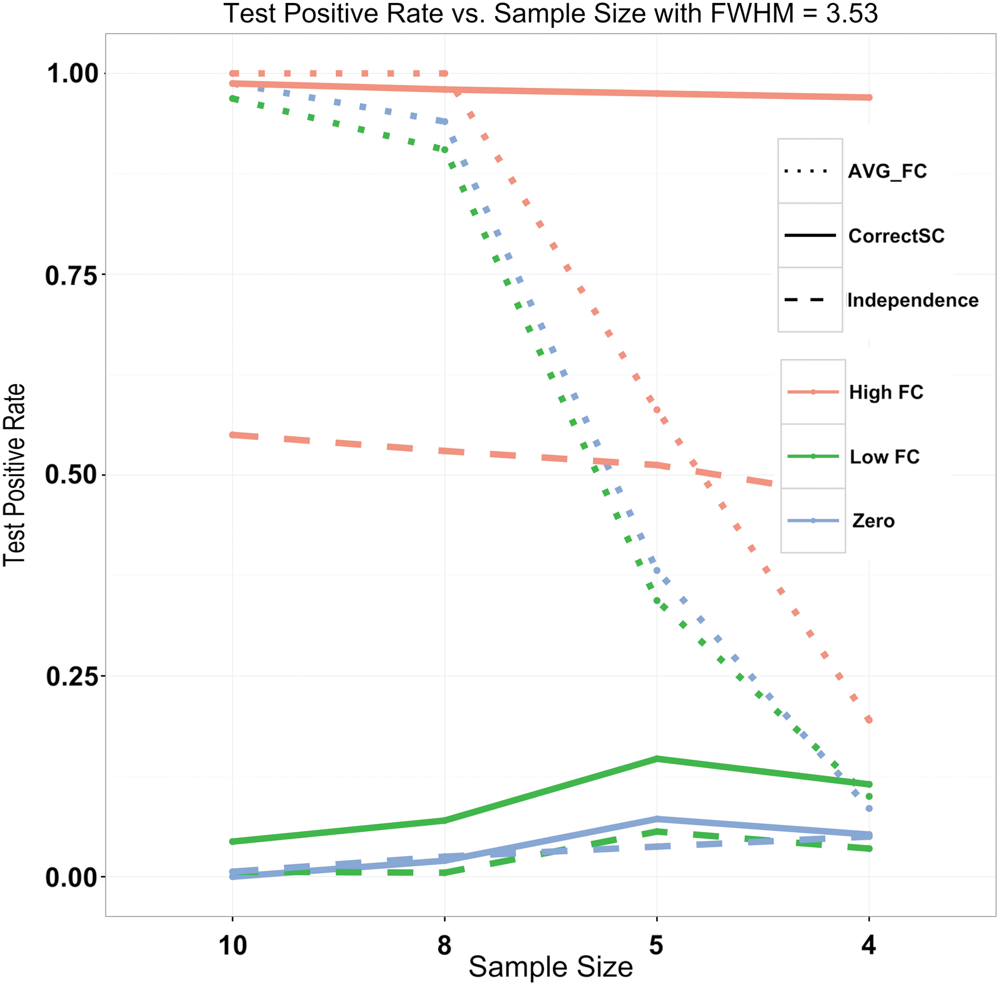
In Figure 1, the rates of positive findings were summarized following three categories of FC: (1) zero FC (i.e., FC = 0, blue) where positive findings were all erroneous, (2) low FC (i.e., FC = 0.1 or 0.2, green) where positive findings may or may not be erroneous, and (3) strong FC (i.e., FC = 0.5 or 0.6, red) where positive findings are desired. As shown in Figure 1, two Bayesian models denoted by solid line (CorrectSC) and dashed line (Independence) are quite robust against data decimation, compared to AVG-FC (dotted line) showing significant decrease in rate of positive findings as decrease in sample size. Moreover, note that high false positive rate is observed with AVG-FC when the underlying true FC = 0, denoted by dotted blue line. When the underlying FC is strong, CorrectSC (solid red line) outperforms the other two approaches but Independence (dashed red) also seems to be very robust to data decimation. With very large sample size, it is expected that the performance of Independence converges to that of CorrectSC, while AVG-FC is more likely to claim all FCs statistically significant.
Test positive rate at different sample sizes with moderate spatial correlation (FWHM = 3.53). Three methods were denoted by different types of line: AVG-FC (dotted line), Bayesian with CorrectSC prior (solid line), and Bayesian with Independence prior (dashed line). Three different colors denote the underlying true strength of FC: red denotes high FC (i.e., FC = 0.5 and 0.6), green denotes low FC (i.e., 0.1 and 0.2), and blue denotes zero FC. FC, functional connectivity.
Data analysis: results
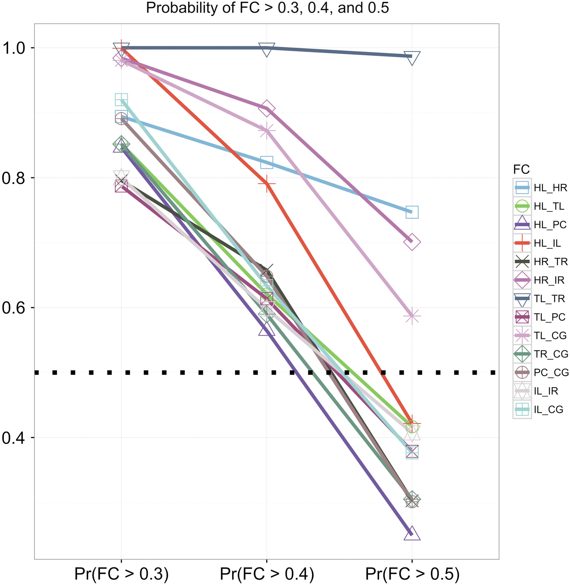
We assessed FC by looking into the following probability: Pr(FC >0.4), where FC denotes the FC estimated by the median value of posterior distribution of each FC. Instead of computing p values based on t-statistics as done for the AVG-FC approach, we computed the posterior probability and used it as an inference tool, that is, any ROI pair with Pr(FC >0.4) >0.5 would be considered important as Xue et al. (2015) used 0.4 as a threshold for moderate or above functional coherence. Although it seems that the threshold values are arbitrary, by generating a series of probabilistic statements with different thresholds such as Pr(FC >0.3), Pr(FC >0.4), and Pr(FC >0.5), we would be able to understand how those probabilities change with different thresholds, indicating which pairs of ROIs are of great interest and importance in terms of rs-FC. The resulting 13 important FC estimates are all above the reference line at Pr(FC >0.4) (Fig. 2 and Table 2).
A graphical summary of 13 important functional connectivity estimates: Probability of FC >0.3, 0.4, and 0.5. The middle dotted line denotes a probability of 0.5. The 13 important pairs are: HL and HR, HL and TL, HL and PC, HL and IL, HR and TR, HR and IR, TL and TR, TL and PC, TL and CG, TR and CG, PC and CG, IL and IR, and IL and CG. CG, cingulate gyrus; HL, left hippocampus; HR, right hippocampus; IL, left insula; IR, right insula; PC, precuneus; TL, left thalamus; TR, right thalamus.
Summary of FC Values with 95% Credible Intervals and Pr(FC > 0.4) for 13 Important ROI Pairs Based on the Bayesian Spatio-Temporal Approach
ROI pairs
FC by Bayesian (95% credible intervals)
Pr (FC >0.4)
FC by AVG-FC (95% confidence intervals)
p values for AVG-FC
Probabilistic SC
HL-HR
0.605 (0.255–0.734)
0.921
0.726 (0.632–0.823)
<0.001
0.093
HL-TL
0.449 (0.150–0.650)
0.594
0.437 (0.235–0.639)
0.003
0.452
HL-PC
0.495 (0.335–0.730)
0.763
0.588 (0.477–0.700)
<0.001
0.105
HL-IL
0.486 (0.366–0.770)
0.820
0.604 (0.461–0.747)
<0.001
0.299
HR-TR
0.466 (0.163–0.637)
0.655
0.472 (0.286–0.656)
0.002
0.427
HR-IR
0.504 (0.336–0.722)
0.786
0.677 (0.574–0.780)
<0.001
0.320
TL-TR
0.674 (0.531–0.809)
1.000
0.842 (0.776–0.907)
<0.001
0.382
TL-PC
0.503 (0.147–0.769)
0.687
0.577 (0.370–0.781)
0.002
0.117
TL-CG
0.521 (0.327–0.797)
0.910
0.662 (0.554–0.768)
<0.001
0.096
TR-CG
0.458 (0.107–0.775)
0.659
0.611 (0.449–0.770)
<0.001
0.112
PC-CG
0.455 (0.322–0.701)
0.832
0.641 (0.513–0.767)
<0.001
0.148
IL-IR
0.429 (0.075–0.755)
0.579
0.678 (0.524–0.833)
<0.001
0.085
IL-CG
0.442 (0.189–0.734)
0.648
0.693 (0.564–0.820)
<0.001
0.028
For comparison, the corresponding FC estimates with 95% confidence intervals and p-values based on the AVG-FC are listed. In the last column, probabilistic structural connectivity values are reported.
CG, cingulate gyrus; HL, left hippocampus; HR, right hippocampus; IL, left insula; IR, right insula; PC, precuneus; ROI, regions of interest; TL, left thalamus; TR, right thalamus.
It is noteworthy that the FC between TL and TR shows the smallest change over the three thresholds, indicating that the FC is quite strong and highly likely to be >0.5. The second strong FC is observed between HL and HR. In contrast, a significant change in probability that the FC between HR and TR, that is, Pr(FC >0.3) = 0.7876 to Pr(FC >0.5) = 0.2633, indicates that the strength of FC between the two ROIs would lie between 0.3 and 0.4 with high probability.
With the AVG-FC approach, all of 28 FC values were statistically significant at FDR = 0.05. As shown in the previous simulation study, the conventional approach tends to result in high false positives because ignoring spatial correlation within a ROI causes to underestimate the variance associated with FC, leading to smaller p values and much tight 95% CI on each FC. In Table 2, 13 important FC values are summarized along with 95% credible intervals and statistics resulted from AVG-FC. Note that 95% CI is always tighter than the corresponding 95% credible interval, because AVG-FC underestimates the variance associated with FC. Probabilistic SC values corresponding to those 13 pairs are also reported in Table 2. Note that HL-HR and TL-TR pairs show the two strongest functional coupling detected by both the conventional approach and our spatiotemporal model. Although the SC for HL-HR (0.093) is much smaller than that for TL-TR (0.382), both pairs are claimed important by our Bayesian approach, indicating that our model can well accommodate both direct and indirect effect of SC on FC estimation.
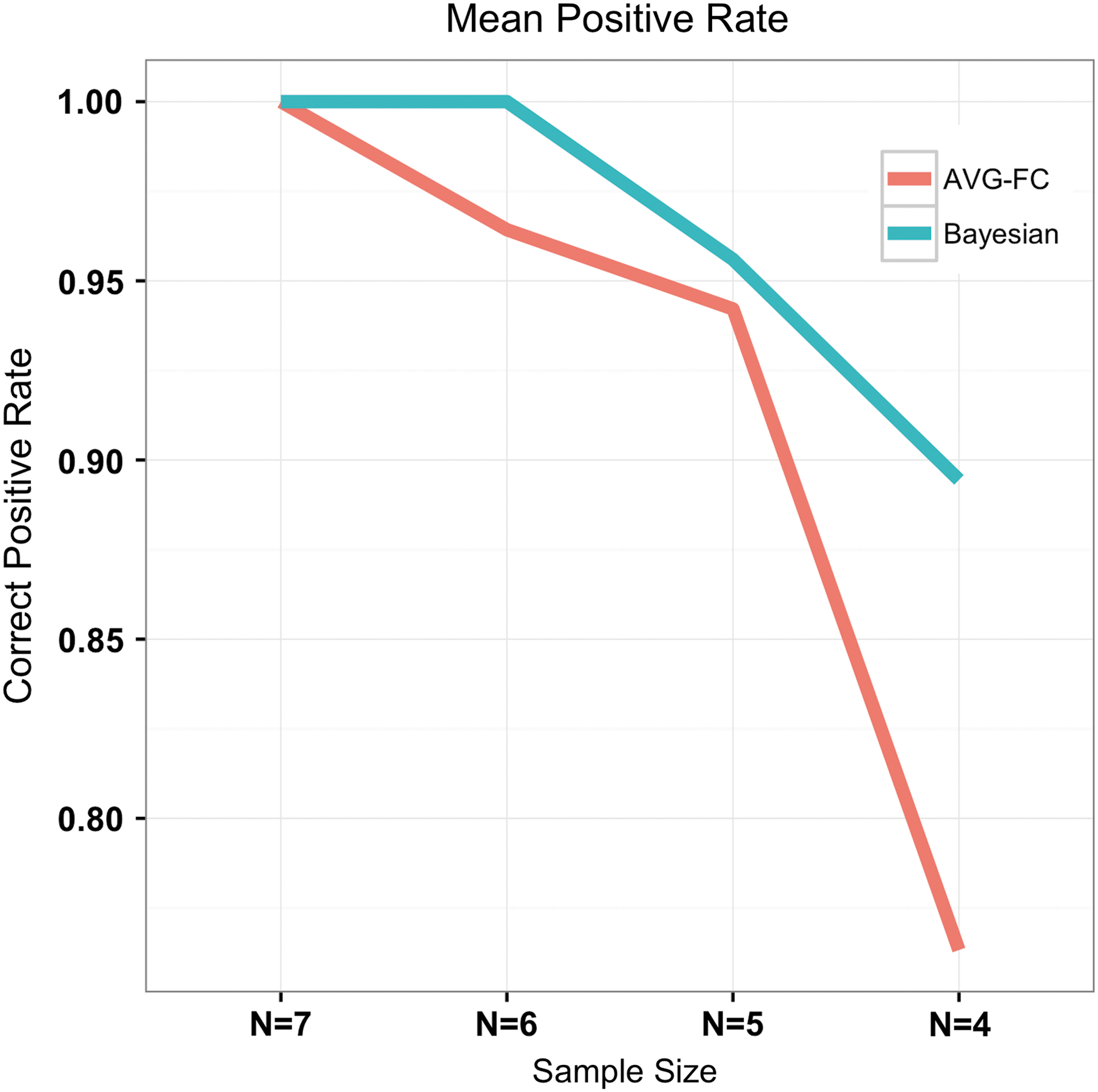
One way to compare methods without knowing the ground truth is to assess how sensitive each method is to data decimation (Yang et al., 2014). If one method is very robust and reliable, then the method is expected to show certain degree of robustness to data decimation, that is, with smaller sample size the method gives rise to the similar results to the original inference result. To this end, we reduced the sample size (n = 6, 5, and 4) with all possible combinations and then analyzed the data with both our Bayesian approach and AVG-FC. With each sample size, we counted how many times the important or statistically significant FC pairs at FDR = 0.05 shown in Table 2 were correctly found by the corresponding method. The results are summarized in Figure 3. It is obvious that our Bayesian spatiotemporal model with double fusion is much more robust to data decimation than AVG-FC. Even with n = 4, on average 89% of the time our approach can result in the same result as n = 7 while only 76% of the time AVG-FC results in the same result as n = 7.
Mean correct positive rates at different sample sizes, n = 7, 6, 5, and 4. “Correct” positive rate denotes how often the 13 FC values summarized in Table 2 were “correctly” detected important by Bayesian spatiotemporal model with double fusion (cyan) and all of 28 FC values were “correctly” classified as significant by AVG-FC (red).
Discussion
We proposed a Bayesian hierarchical spatiotemporal model with double fusion to analyze multimodal neuroimaging data, that is, concurrently acquired rs-fMRI and DTI data, which could properly take into account the intrinsic spatial correlation among voxels within an ROI, and temporal correlation at each voxel. Accounting for those underlying correlation enables us to draw a valid inference about between-ROI functional couplings. Using a Bayesian analytic approach, it is very natural to combine prior knowledge about the SC based on DTI data with rs-fMRI data for updating posterior information about the FC between ROIs. Moreover, accounting for the role of direct and indirect association between FC and SC through double fusion provides a unified framework for incorporating multimodal MRI data. Our model is flexible enough to be modified to accommodate longitudinal or task-induced fMRI data.
We validated our approach using stimulation study and also applied our model to analyze multimodal MRI data to assess the impact of the SC between brain regions on rs-FC. The simulation study showed that an informative prior based on the SC reduced the MSE of FC estimates, compared to using a prior based on structural independence. In addition, it showed that failing to take into account the underlying spatial correlation within an ROI highly inflated false positive rates, leading to erroneous conclusions, for example, tight 95% confidence intervals. The similar finding was reported with task-induced fMRI analysis (Kang et al., 2012).
In data analysis, 13 ROI pairs show important functional couplings in the brain network through our Bayesian approach, whereas all 28 ROI pairs were claimed statistically significant through AVG-FC, although it might be false positive findings. When we considered more conservative threshold such as Pr (FC >0.5) >0.5, then only four ROI pairs remained as important: HL-HR, HR-IR, TL-TR, and TL-CG. We were also able to show that our Bayesian spatiotemporal model was much robust to data decimation, which would be one of the most desirable properties of statistical models. Although the data decimation approach would be more meaningful when we had a large sample size, it would be still valid to show that our approach was more robust than AVG-FC with such small sample size.
Our model requires estimating parameters using MCMC methods, which in general are more computationally demanding than frequentist methods, for example, AVG-FC and require the convergence of the MCMC chains that is always challenging. In this study, we confirmed the convergence by the Gelman–Rubin diagnostic (Gelman and Rubin, 1992): the diagnostic values associated with our simulation studies and data analysis were <1.2. However, the Bayesian framework allows us to easily combine two distinct sources of information to estimate FC with higher precision and accuracy as measured by MSE. Moreover, we were able to obtain a smaller MSE using the informative prior based on DTI data.
Then one can argue that our approach heavily relies on the assumption that we have good estimates of the SC. As shown in the simulation study, reliable prior structural information that is somewhere between true underlying SC and structural independence SC can reduce the MSE of estimates. However, if the prior information is incorrect but we have a large sample size, which can be true in fMRI data analysis, then the point estimates of interest would not be heavily affected using an incorrect prior. But the variance of the estimates will increase and the time to attain the convergence of Markov chains may also increase.
Conclusion
In summary, we proposed a novel Bayesian spatiotemporal model with double fusion to better estimate FC using both rs-fMRI and DTI data. The main advantages of using our model relative to current standard methodologies are: (1) It is a novel approach that combines multimodal data producing estimates of FC with lower MSEs in simulation. (2) It gives valid inference about ROI-level FC while properly accounting for underlying spatiotemporal correlations. (3) It characterizes a probability distribution of each FC estimate, which is a unique feature of a Bayesian approach. (4) It can incorporate both direct and indirect effects of SC on FC estimation. (5) It provides an inference tool that is much more robust to data decimation compared to the conventional approach.
Footnotes
Acknowledgments
The authors thank Drs. David Degras (University of Massachusetts), Mark Fiecas (University of Minnesota), and Baxter Rogers (Vanderbilt University) for helpful discussions. This work was, in part, supported by NIH (Grant No. R01 NS075270).
Author Disclosure Statement
No competing financial interests exist.
References
1.
AltinayMI, HulvershornLA, KarneH, BeallEB, AnandA. 2016. Differential Resting-State Functional Connectivity of Striatal Subregions in Bipolar Depression and Hypomania. Brain Connect, 6:255–265.
BehrensTE, BergHJ, JbabdiS, RushworthMF, WoolrichMW. 2007. Probabilistic diffusion tractography with multiple fibre orientations: what can we gain?. Neuroimage, 34:144–155.
4.
BehrensTE, WoolrichMW, JenkinsonM, Johansen-BergH, NunesRG, ClareS, et al.2003. Characterization and propagation of uncertainty in diffusion-weighted MR imaging. Magn Reson Med, 50:1077–1088.
5.
BowmanFD. 2007. Spatiotemporal models for region of interest analyses of functional neuroimaging data. J Am Stat Assoc, 102:442–453.
6.
BowmanFD, ZhangL, DeradoG, ChenS. 2012. Determining functional connectivity using fMRI data with diffusion-based anatomical weighting. NeuroImage, 62:1769–1779.
7.
CordesD, HaughtonVM, ArfanakisK, CarewJD, TurskiPA, MoritzCH, et al.2001. Frequencies contributing to functional connectivity in the cerebral cortex in “resting-state” data. AJNR Am J Neuroradiol, 22:1326–1333.
8.
CressieNAC. 1993. Statistics for Spatial Data. New York: Wiley.
DecoG, McIntoshAR, ShenK, HutchisonRM, MenonRS, EverlingS, et al.2014. Identification of optimal structural connectivity using functional connectivity and neural modeling. J Neurosci, 34:7910–7916.
11.
DicksteinDP, GorrostietaC, OmbaoH, GoldbergLD, BrazelAC, GableCJ, et al.2010. Fronto-temporal spontaneous resting state functional connectivity in pediatric bipolar disorder. Biol Psychiatry, 68:839–846.
12.
FristonKJ, FrackowiakRSJ, LiddlePF, FrithCD. 1993. Functional connectivity: the principal-component analysis of large (PET) data sets. J Cereb Blood Flow Metab, 13:5–14.
13.
GelmanA, RubinDB. 1992. Inference from iterative simulation using multiple sequences. Statist Sci, 7:457–511.
14.
GloverGH, LiTQ, RessD. 2000. Image-based method for retrospective correction of physiological motion effects in fMRI: RETROICOR. Magn Reson Med, 44:162–167.
15.
GreiciusMD, SupekarK, MenonV, DoughertyRF. 2009. Resting-state functional connectivity reflects structural connectivity in the default mode network. Cereb Cortex, 19:72–78.
16.
HagmannP, CammounL, GigandetX, MeuliR, HoneyCJ, WedeenVJ, et al.2008. Mapping the structural core of human cerebral cortex. PLoS Biol, 6:e159.
17.
HansenEC, BattagliaD, SpieglerA, DecoG, JirsaVK. 2015. Functional connectivity dynamics: modeling the switching behavior of the resting state. Neuroimage, 105:525–535.
18.
HarrisonSJ, WoolrichMW, RobinsonEC, GlasserMF, BeckmannCF, JenkinsonM, et al.2015. Large-scale probabilistic functional modes from resting state fMRI. NeuroImage, 109:217–231.
19.
HendlerT, PiankaP, SigalM, KafriM, Ben-BashatD, ConstantiniS, et al., 2003. Two are better than one: combining fMRI and DTI based fiber tracking for effective pre-surgical mapping. Proc Int Soc Magn Reson Med, p. 394.
20.
HolmesMJ, YangX, LandmanBA, DingZ, KangH, Abou-KhalilB, et al.2013. Functional networks in temporal-lobe epilepsy: a voxel-wise study of resting-state functional connectivity and gray-matter concentration. Brain Connect, 3:22–30.
21.
HoneyCJ, SpornsO, CammounL, GigandetX, ThiranJP, MeuliR, et al.2009. Predicting human resting-state functional connectivity from structural connectivity. Proc Natl Acad Sci USA, 106:2035–2040.
22.
HuangH, DingM. 2016. Linking functional connectivity and structural connectivity quantitatively: a comparison of methods. Brain Connect, 6:99–108.
23.
JooSH, LimHK, LeeCU. 2016. Three large-scale functional brain networks from resting-state functional MRI in subjects with different levels of cognitive impairment. Psych Invest, 13:1–7.
24.
KangH, OmbaoH, LinkletterC, LongN, BadreD. 2012. Spatio-spectral mixed effects model for functional magnetic resonance imaging data. J Am Stat Assoc, 107:568–577.
25.
MeierJ, TewarieP, HillebrandA, DouwL, van DijkBW, StufflebeamSM, et al.2016. A mapping between structural and functional brain networks. Brain Connect, 6:298–311.
26.
MorganVL, MishraA, NewtonAT, GoreJC, DingZ. 2009. Integrating functional and diffusion magnetic resonance imaging for analysis of structure-function relationship in the human language network. PLoS One, 4:e6660.
27.
OlesenP, NagyZ, WesterbergH, KlingbergT. 2003. Combined analysis of DTI and fMRI data reveals a joint maturation of white and grey matter in a fronto-parietal network. Cogn Brain Res, 8:48–57.
28.
PatilA, HuardD, FonnesbeckCJ. 2010. PyMC: Bayesian stochastic modelling in python. J Stat Softw, 35:1–81.
29.
PoldrackRA, MumfordJA, NicholsTE. 2011. Handbook of Functional MRI Data Analysis. New York, NY: Cambridge University Press.
30.
SchmittmannVD, JahfariS, BorsboomD, SaviAO, WaldorpLJ. 2015. Making large-scale networks from fMRI data. PLoS One, 10:e0129074.
31.
van den HeuvelMP, MandlRC, KahnRS, Hulshoff PolHE. 2009. Functionally linked resting-state networks reflect the underlying structural connectivity architecture of the human brain. Hum Brain Mapp, 30:3127–3141.
32.
WangK, LiangM, WangL, TianL, ZhangX, LiK, et al.2007. Altered functional connectivity in early Alzheimer's disease: a resting-state fMRI study. Hum Brain Mapp, 28:967–978.
33.
WerringDJ, ClarkCA, BarkerGJ, MillerDH, ParkerGJ, BrammerMJ, et al.1998. The structural and functional mechanisms of motor recovery: complementary use of diffusion tensor and functional magnetic resonance imaging in a traumatic injury of the internal capsule. J Neurol Neurosurg Psychiatry, 65:863–869.
34.
WieshmannUC, KrakowK, SymmsMR, ParkerGJ, ClarkCA, BarkerGJ, et al.2001. Combined functional magnetic resonance imaging and diffusion tensor imaging demonstrate widespread modified organisation in malformation of cortical development. J Neurol Neurosurg Psychiatry, 70:521–523.
35.
WorsleyKJ, MarrettS, NeelinP, VandalAC, FristonKJ, EvansAC. 1996. A unified statistical approach for determining significant signals in images of cerebral activation. Hum Brain Mapp, 4:58–73.
36.
XueW, BowmanFD, PileggiAV, MayerAR. 2015. A multimodal approach for determining brain networks by jointly modeling functional and structural connectivity. Front Comput Neurosci, 9:1–11.
37.
YangX, KangH, NewtonAT, LandmanBA. 2014. Evaluation of statistical inference on empirical resting state fMRI. IEEE Trans Biomed Eng, 61:1091–1099.
38.
YuZ, PradoR, QuinlanEB, CramerSC, OmbaoH. 2016. Understanding the impact of stroke on brain motor function: a hierarchical Bayesian approach. J Am Stat Assoc, 111:549–563.
39.
ZhangL, GuindaniM, VannucciM. 2015. Bayesian models for fMRI data analysis. Wiley Interdiscip Rev Comput Stat, 7:21–41.
40.
ZhangL, GuindaniM, VersaceF, VannucciM. 2014. A spatio-temporal nonparametric Bayesian variable selection model of fMRI data for clustering correlated time courses. NeuroImage, 95:162–175.
41.
ZhuD, ZhangT, JiangX, HuX, ChenH, YangN, et al.2014. Fusing DTI and fMRI data: a survey of methods and applications. Neuroimage, 102:184–191.
42.
ZippoAG, CastiglioniI, BorsaVM, BiellaGE. 2015. The compression flow as a measure to estimate the brain connectivity changes in resting state fMRI and 18FDG-PET Alzheimer's disease connectomes. Front Comput Neurosci, 9:148.