Accounting for Non-Gaussian Sources of Spatial Correlation in Parametric Functional Magnetic Resonance Imaging Paradigms I: Revisiting Cluster-Based Inferences

Abstract

In a recent study, Eklund et al. employed resting-state functional magnetic resonance imaging data as a surrogate for null functional magnetic resonance imaging (fMRI) datasets and posited that cluster-wise family-wise error (FWE) rate-corrected inferences made by using parametric statistical methods in fMRI studies over the past two decades may have been invalid, particularly for cluster defining thresholds less stringent than p < 0.001; this was principally because the spatial autocorrelation functions (sACF) of fMRI data had been modeled incorrectly to follow a Gaussian form, whereas empirical data suggested otherwise. Here, we show that accounting for non-Gaussian signal components such as those arising from resting-state neural activity as well as physiological responses and motion artifacts in the null fMRI datasets yields first- and second-level general linear model analysis residuals with nearly uniform and Gaussian sACF. Further comparison with nonparametric permutation tests indicates that cluster-based FWE corrected inferences made with Gaussian spatial noise approximations are valid.

Introduction

Blood oxygenation level dependent (BOLD) functional magnetic resonance imaging (fMRI) has been the pre-eminent technique to study brain function and pathology over the past two decades (Buxton, 2009). The preponderance of fMRI studies on brain function over this period has adopted parametric statistical methods under the general linear model (GLM) framework to assess brain activation during cognitive (Moffett et al., 2015), affective (Lebois et al., 2015), sensory (Gopinath et al., 2012; Sathian et al., 2011), or motor tasks (McGregor et al., 2015).

Recently, the validity of cluster-based family-wise error (FWE)-corrected inferences made in many of these studies have been called into question by Eklund et al. (2016), who reported that the main source of these incorrect inferences was that the spatial autocorrelation function (sACF) of the fMRI data had been assumed to be Gaussian and uniform across the brain (Forman et al., 1995; Kiebel et al., 1999), whereas empirical data suggest otherwise (Carmack et al., 2012; Eklund et al., 2016). This is reflected in the residuals of the GLM analysis possessing considerable heterogeneity in smoothness across the brain, as well as non-Gaussian sACFs.

Eklund et al. (2016) suggested that the spatial correlation in fMRI data that causes a heavy-tailed behavior in sACF is induced in good part by the MRI systems hardware (Kriegeskorte et al., 2008; Weisskoff, 1996). However, it is more likely that the non-Gaussianity of the sACF as well as nonuniform smoothness of the GLM residuals is caused by non-Gaussian signal sources: resting-state brain function networks (Smith et al., 2009), physiological processes as well as artifacts related to motion, and acquisition and reconstruction of echo planar imaging (EPI) data employed in fMRI studies.

Relatedly, the brain areas with the highest range of local spatial correlation in the fMRI datasets reported by Eklund et al. (2016) (e.g., see supplementary fig. 19 of that paper) coincide with what are considered hubs of functional connectivity networks, for example, posterior cingulate cortex (Buckner et al., 2009). Physiological processes such as cardiac (Chang et al., 2009; Dagli et al., 1999; Glover et al., 2000) and respiratory (Birn et al., 2006; Glover et al., 2000) fluctuations can introduce spatial correlations into fMRI time series. Motion artifacts and image acquisition artifacts also have non-Gaussian characteristics that serve as a basis for some data analysis techniques such as independent component analysis (ICA) that have been developed to remove such artifacts (Pruim et al., 2015; Salimi-Khorshidi et al., 2014).

Hence, accounting for these sources of non-Gaussian signal during parametric analysis of fMRI paradigms could result in GLM residuals with uniform and Gaussian sACF.

In this first of a two-part study, we show that estimating non-Gaussian signal components from the resting-state fMRI null datasets renders spatial correlation of the GLM residuals of both first- and second-level analysis nearly uniform and Gaussian, and the inferences based on Gaussian spatial noise approximations are rendered valid. In the companion paper (Gopinath et al., 2017), we apply the results of this exercise to a common visual processing fMRI paradigm.

Materials and Methods

Participants

Twenty healthy, right-handed participants were recruited from the Atlanta metropolitan area (10 male and 10 female; median age = 22 years). Exclusion criteria for the study were: pregnancy, metallic implants, or other contraindication to MRI; history of psychiatric illness or substance abuse or dependence; significant family history of psychiatric or neurological illness; current use of any centrally acting medications; and serious medical or neurological illness. Since caffeine can alter neural (Nehlig and Boyet, 2000) as well as fMRI BOLD responses (Liau et al., 2008) and is also known to reduce the strength of rsfMRI networks in other areas (Rack-Gomer et al., 2009), participants were asked to refrain from ingesting caffeine products for 12 h before the scan. Written informed consent was obtained from participants under an IRB-approved protocol.

Experimental design

Each participant took part in a 10-min resting-state fMRI scan. The participants were instructed to keep their eyes open and blink at a normal rate during the resting-state scans, since the eyes-open condition best engenders a neutral affective and attentional state (Gopinath et al., 2011) and exhibits stronger resting-state fMRI (rsfMRI) networks than the eyes-closed condition (Van Dijk et al., 2010).

Image acquisition

MRI images were acquired on a 3T Siemens TIM Trio scanner with a 12-channel receiver array head coil. BOLD fMRI scans were acquired with a gradient echo EPI sequence. For the resting-state fMRI scans, the imaging parameters were: field-of-view (FOV) = 220 mm; repetition time (TR)/echo time (TE) = 3000/25 ms flip angle (FA) = 90°; 74 × 74 matrix size; bandwidth = 2598 Hz/pixel; 48 interleaved axial slices of 3 mm width covering the whole brain; and 192 scan volumes. Prospective real-time motion correction (Thesen et al., 2000) was employed with all EPI scans to minimize motion artifacts. Also, a whole-brain 3D T1-weighted MPRAGE sequence (FOV = 230 mm; TR/TI/TE/FA = 2250 ms/900 ms/3 ms/9°; 0.9 × 0.9 × 1 mm resolution; TI = inversion time) was acquired to provide anatomic detail. All these scans were acquired with parallel imaging: GRAPPA acceleration factor = 2; 24 (36 for MPRAGE) phase-encoding reference lines. Foam padding was provided to minimize head motion.

Null dataset simulated fMRI paradigm

Since block fMRI paradigms have been shown to be the most sensitive to inflated false positives while employing cluster-based methods to correct for FWE (Cox et al., 2017; Eklund et al., 2016), a “standard” block fMRI paradigm consisting of 22 alternating blocks of 12 sec rest and 12 sec activation (where the activation blocks alternated between two types of stimuli: BlockA and BlockB) was chosen to assess spatial correlation of GLM residuals.*

Data analysis

Data analysis was performed by using the AFNI (Cox, 1996) and FSL (Smith et al., 2004) software packages and in-house programs written in Matlab (MathWorks, Natick, MA). The resting-state fMRI datasets from the 21 subjects were used to generate null datasets. The spatial correlation of the first- and second-level residuals (obtained from GLM analysis of the simulated block fMRI paradigm) was assessed, before and after removal of non-Gaussian signal sources in null rsfMRI datasets through a principal component analysis (PCA)-based technique.

Pre-processing

The rsfMRI voxel time series were temporally shifted to account for differences in slice acquisition times, 3D volume registered to a base volume to account for global rigid motion, co-registered to the T1-weighted high-resolution anatomic scan and spatially normalized to the MNI152 template, resampled to 3 × 3 × 3 mm voxel resolution, detrended of fifth-order polynomial drifts, and spatially smoothed with an isotropic Gaussian kernel with full-width at half maximum (FWHM) = 5 mm (and 8 mm in a separate analysis; see Effects of Increased Spatial Smoothing section Supplementary Data, including Supplementary Figures S1–S3, and Supplementary Tables S1–S4; Supplementary Data are available online at www.liebertpub.com/brain).

Creation of rsfMRI-based null datasets

The spatially smoothed rsfMRI time series described earlier served as the commonly used null fMRI datasets (Cox et al., 2017; Eklund et al., 2016). The aim of this proof-of-concept study was to examine the hypothesis that nonuniform and non-Gaussian spatial correlation in fMRI datasets arises from a set of non-Gaussian (neural as well as artifactual) signal sources, which when removed from the datasets will leave the spatial correlation nearly uniform and Gaussian. To this end, the four-dimensional (4D) rsfMRI dataset (REST) for each subject was decomposed with PCA using the 3dpc program in the AFNI software suite (Cox, 1996) into N 3D spatial principal components (PCs) along with N orthogonal 1D Eigen time series, ranked from the highest to the lowest Eigenvalue, where N is the length of the rsfMRI time series. After this, the signals proportional to the Eigen time series associated with the top 40, 110, 130, 150, and 170 PCs were removed (through multiple linear regression) from the rsfMRI data to create different PC-detrended null fMRI datasets (e.g., REST-dt40PC) for GLM analysis, to examine the effects of different degrees of PC detrending on the spatial correlation of null fMRI data, as well as GLM analysis residuals.

First-level analysis: block fMRI paradigm

For each subject, voxel time series from each of the null fMRI datasets were modeled as the sum of the convolutions of the two stimulus design vectors (one each for BlockA and BlockB; the vectors comprised “1” sec for the duration of activation blocks and “0” sec during rest) with 1-free parameter (amplitude) gamma-variate impulse response function, with a GLM under the multiple linear regression-based framework. The first-level GLM analysis on the original rsfMRI null dataset (REST) employed generalized least squares and ARMA(1,1) prewhitening to account for temporal correlation (employing AFNI programs 3dDeconvolve and 3dREMLfit). Since the process of detrending the top PCs from the rsfMRI likely engenders effective prewhitening of temporal correlation, the first-level GLM analysis on the PC-detrended null datasets (e.g., REST-dt40PC) was carried out with an ordinary least-squares method (using 3dDeconvolve). The GLM-estimate amplitude “β” coefficient for each block type (BlockA and BlockB) expressed the activation in response to the corresponding stimulus.

Second-level analysis

Group-level t-test maps for BlockA and BlockB conditions as well as BlockA versus BlockB t-contrast maps on first-level GLM-estimate amplitudes (βs) were computed with the 3dttest++ (which also performs ordinary least-squares regression analysis) program in AFNI.

Second-level analysis: multiple-comparison corrected inference

Group-statistical parametric maps were clustered and the significance of activations, accounting for multiple comparisons, was derived in two different ways.

The first method estimated FWE-corrected inferences based on Monte Carlo (MC) simulation of the process of image generation, estimated spatial correlation of voxels, intensity thresholding, masking (whole-brain), and cluster identification (Cox et al., 2017) through the 3dClustSim program implemented in AFNI. In this study, two voxels were assumed to belong to the same cluster if they survived the uncorrected p-value threshold and the voxels shared a face. The uncorrected p-value threshold selected is termed cluster defining threshold (CDT) in this article. The CDT was varied over a number of pre-specified values between p < 0.05 and p < 0.001 and the minimum cluster size needed to adjudge the cluster-level activation significant at different prespecified FWE rates (α values) was computed. The spatial correlation among voxels in the random noise fields used during MC simulations was quantified by the sACF parameters (see Estimation of spatial correlation) estimated from the residuals of second-level GLM analysis.

The second method is a variation of the nonparametric approach favored by Eklund et al. (2016), since it is independent of the spatial noise structure of the residuals. In this method, implemented as an optional feature in AFNI's 3dttest++ program (Cox et al., 2017), a permutation null distribution was generated by randomizing among the subjects the signs of the voxel-wise residuals of the second-level GLM, and the t-tests were repeated. The null permutation distribution of t-maps generated by 10,000 such iterations was used to estimate minimum cluster-size thresholds for cluster-based FWE correction at different CDTs and α-values.

Estimation of spatial correlation

The spatial correlation of each of the null fMRI datasets as well as the 4D first- and second-level GLM residuals datasets was quantified by the parameters of the sACF. The sACF parameters for all datasets were estimated at both the whole-brain level (across all voxels in the brain) and within spherical local neighborhoods of 25–60 mm (depending on the shape of the empirical local sACF) radius using the 3dFWHMx program in AFNI that expresses sACF as a mixed Gaussian + mono-exponential model, to account for longer tails in the shape of the empirical sACFs seen in fMRI data than a pure squared-exponential model can accommodate (Cox et al., 2017). \documentclass{aastex}\usepackage{amsbsy}\usepackage{amsfonts}\usepackage{amssymb}\usepackage{bm}\usepackage{mathrsfs}\usepackage{pifont}\usepackage{stmaryrd}\usepackage{textcomp}\usepackage{portland, xspace}\usepackage{amsmath, amsxtra}\usepackage{upgreek}\pagestyle{empty}\DeclareMathSizes{10}{9}{7}{6}\begin{document} \begin{align*} sACF = a \times \exp \left( { - { \frac { { r^2 } } { 2 { b^2 } } } } \right) + \left( { 1 - a } \right) \times \exp \left( { - \frac { r } { c } } \right) , \tag { 1 } \end{align*} \end{document}

where r is the distance from a given voxel, and a is the parameter that expresses the mixture of Gaussian and mono-exponential portions of the sACF. The parameter a \documentclass{aastex}\usepackage{amsbsy}\usepackage{amsfonts}\usepackage{amssymb}\usepackage{bm}\usepackage{mathrsfs}\usepackage{pifont}\usepackage{stmaryrd}\usepackage{textcomp}\usepackage{portland, xspace}\usepackage{amsmath, amsxtra}\usepackage{upgreek}\pagestyle{empty}\DeclareMathSizes{10}{9}{7}{6}\begin{document}$$\in$$ \end{document} (0,1), but it is constrained to vary between 0.06 and 0.994 by the nonlinear optimization algorithm used by AFNI to estimate the spatial correlation of the data. A high value of a will indicate that sACF was nearly Gaussian. The parameters b and c together quantify the spatial smoothness (FWHM) of the data, are constrained to be positive (b, c > 0), and reflect the smoothness of the Gaussian and mono-exponential components respectively. Further, the apparent FWHM (FWHM_ap) of the empirical auto-correlation function was obtained for all datasets (both at whole-brain level and within 25–60 mm radius spherical local neighborhoods).

Results

Revisiting cluster-based inference

Effects of PC detrending on spatial correlation of null rsfMRI datasets

Table 1 lists the estimated (across all voxels in the brain) average (across 21 subjects) sACF parameters as well as empirical spatial smoothness (FWHM_ap) of the rsfMRI datasets (REST) and other null datasets (REST-dt40PC, REST-dt110PC, etc.) generated by detrending different numbers of PCs. The spatial correlation decreased and became more Gaussian progressively as the number of PCs detrended increased. For each subject, an ideal set of null fMRI datasets (REST-dtPC_opt) was formed by selecting the minimum number of PCs (among those described earlier), N_opt, required to obtain a PC-detrended dataset that exhibited Gaussian sACF (i.e., for which the sACF Gaussianity parameter a, reached its maximum (algorithm constrained) value of 0.9940). Individually, apart from two subjects with N_opt = 150 PCs, and two with N_opt = 120 PCs, all the other subjects' null datasets exhibited Gaussian sACF after the first 110 PCs were detrended from the rsfMRI datasets. Figure 1 plots the average (across 21 subjects) Eigen spectrum of the PCs. On average, the first 110 PCs accounted for around 90% of the variance in the 4D rsfMRI data. However, as mentioned earlier, N_opt had to be determined separately for each subject to ensure adequate removal of non-Gaussian signals in the data.

FIG. 1.

Plot of cumulative variance (0.2 to 1 ≡ 20–100%) explained by considering increasing number of PCs, averaged across 21 subjects. The error bars reflect standard error across 21 subjects. PCs, principal components.

Table 1.

The Group Average Estimated Spatial Autocorrelation Function Parameters (Assuming Mixed-Model Spatial Autocorrelation Functions) and the Empirical Spatial Smoothness (FWHM_ap) of the Different Null Functional Magnetic Resonance Imaging Datasets (Mean Across 21 Subjects ± Standard Deviation)

Null datasets	ACF a	ACF b	ACF c	FWHM_ap (mm)
REST	0.610 ± 0.043	4.234 ± 0.100	13.165 ± 1.198	11.39 ± 0.38
REST-dt40PC	0.909 ± 0.028	3.986 ± 0.051	8.047 ± 0.391	9.47 ± 0.12
REST-dt110PC	0.992 ± 0.005	3.812 ± 0.043	5.520 ± 3.841	8.97 ± 0.10
REST-dt130PC	0.993 ± 0.003	3.799 ± 0.045	5.999 ± 4.036	8.94 ± 0.10
REST-dt150PC	0.994 ± 0.000	3.786 ± 0.044	4.071 ± 2.106	8.90 ± 0.10
REST-dt170PC	0.994 ± 0.000	3.722 ± 0.040	2.886 ± 0.479	8.75 ± 0.10

ACF, autocorrelation function.

Effects of PC detrending on spatial correlation of residuals

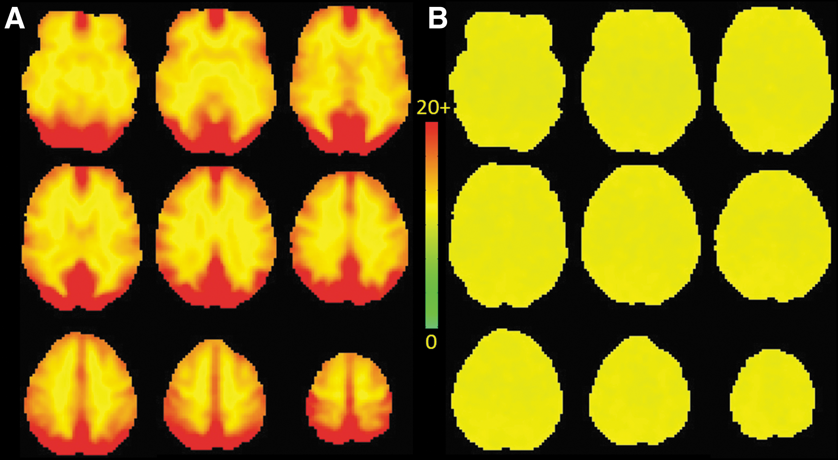
PC detrending rendered the spatial correlation of residuals of GLM nearly Gaussian and uniform across the brain. Table 2 lists the estimated whole-brain sACF parameters as well as spatial smoothness (FWHM_ap) of the residuals of the second-level GLM (BlockA–BlockB paired t-test) analysis obtained from REST, as well as the second-level GLM residuals obtained from PC-detrended null datasets (REST-dt40PC, REST-dt110PC, etc.). The second-level residuals from the REST dataset exhibited non-Gaussian sACF (Table 2) and also exhibited significant heterogeneity in spatial smoothness and the sACF Gaussianity parameter across the brain (Figs. 2A and 3A). Detrending the increasing number of principal components from the null REST datasets led to the second-level residuals exhibiting decreased spatial correlation, increased Gaussianity as quantified by the sACF a parameter, as well as increased homogeneity in spatial smoothness of the second-level GLM residuals (Table 2; also see Figs. 2 and 3). In fact, the sACF a parameter that quantifies the Gaussian part of the mixed noise sACF model reached its maximum (algorithm constrained) value of 0.994 (up to three significant figures) when the top 110 or higher number of PCs were detrended from all the REST datasets. Figures 2B and 3B display the local spatial smoothness and the sACF Gaussianity parameter across the brain of the second-level residuals obtained from the REST-dtPC_opt null dataset. The spatial correlations of these residuals were nearly uniform and Gaussian across the brain.

FIG. 2.

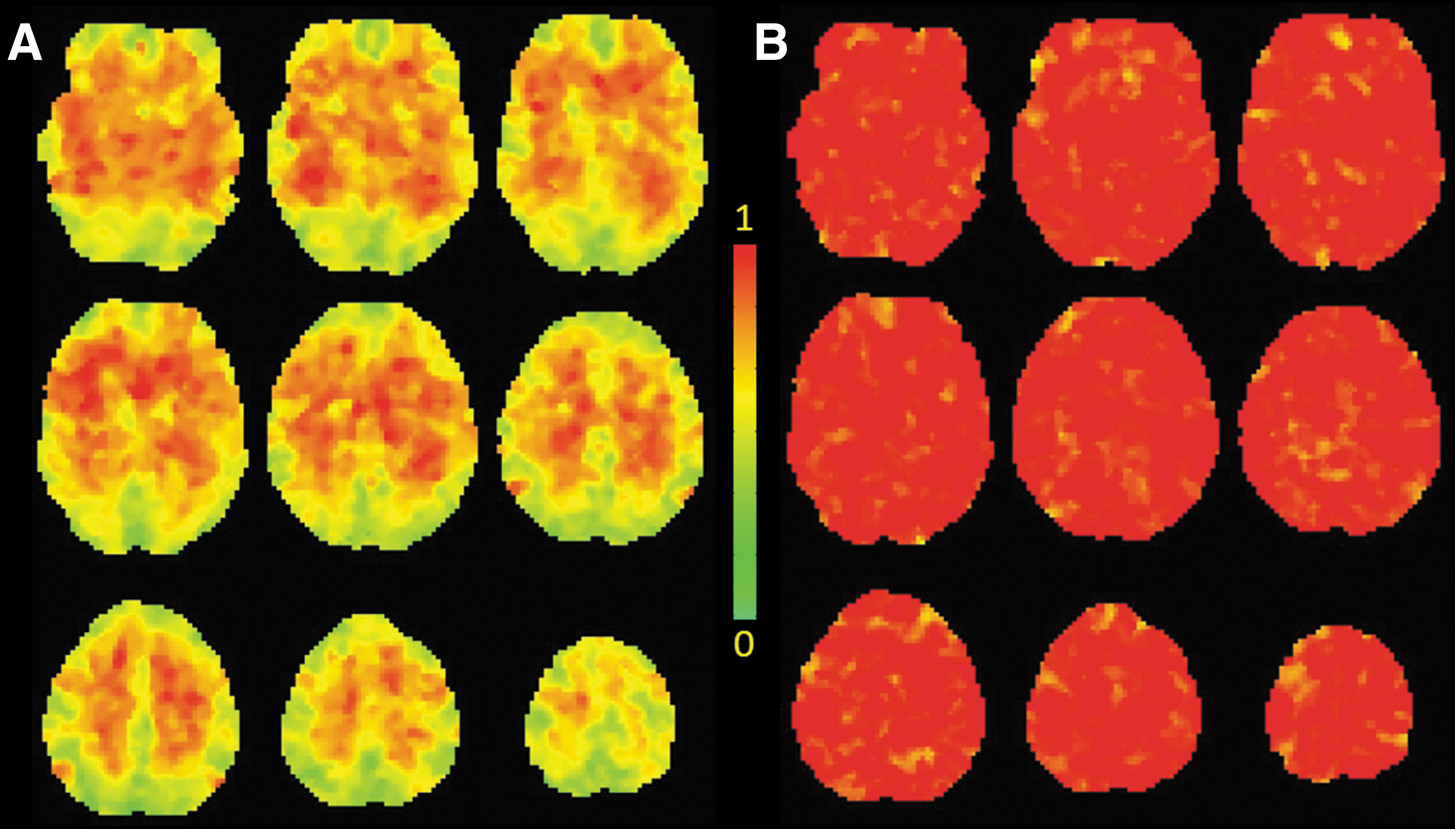
Maps of local spatial smoothness (FWHM_ap) across the brain of the second-level analysis GLM residuals obtained from (A) REST and (B) REST-dtPC_Opt datasets. Left hemisphere is on the right side of the images. GLM, general linear model.

FIG. 3.

Maps of the local sACF a parameter (which quantifies the Gaussian component of sACF) across the brain of the second-level analysis GLM residuals obtained from (A) REST and (B) REST-dtPC_Opt datasets. Left hemisphere is on the right side of the images. sACF, spatial autocorrelation functions.

Table 2.

The Estimated Spatial Autocorrelation Function Parameters (Assuming Mixed-Model Spatial Autocorrelation Functions) and the Corresponding Empirical Spatial Smoothness (FWHM_ap) of the Residuals of Second-Level BlockA Versus BlockB Group t-Test Analysis Conducted on the Corresponding Condition Amplitude (Estimated βs), Employing the Original Null Datasets (REST) as Well as the Null Datasets Obtained by Detrending Different Numbers of PCs from the REST Datasets (e.g., REST-dt40PC) the Numbers in the Parenthesis Are the Average (Across 21 Subjects) Value of the Spatial Autocorrelation Functions Parameters and Empirical FWHM_ap for the Residuals from First-Level General Linear Model Analysis

Null datasets	ACF a	ACF b	ACF c	FWHM_ap (mm)
REST	0.571 (0.613)	4.222 (4.234)	14.04 (13.196)	11.73 (11.38)
REST-dt40PC	0.896 (0.909)	4.010 (3.986)	7.934 (8.045)	9.53 (9.47)
REST-dt110PC	0.994 (0.992)	3.775 (3.812)	2.934 (5.620)	8.87 (8.97)
REST-dt130PC	0.994 (0.993)	3.778 (3.799)	3.044 (5.962)	8.88 (8.94)
REST-dt150PC	0.994 (0.994)	3.790 (3.786)	2.888 (3.990)	8.91 (8.90)
REST-dt170PC	0.994 (0.994)	3.727 (3.723)	2.7908 (2.785)	8.76 (8.75)

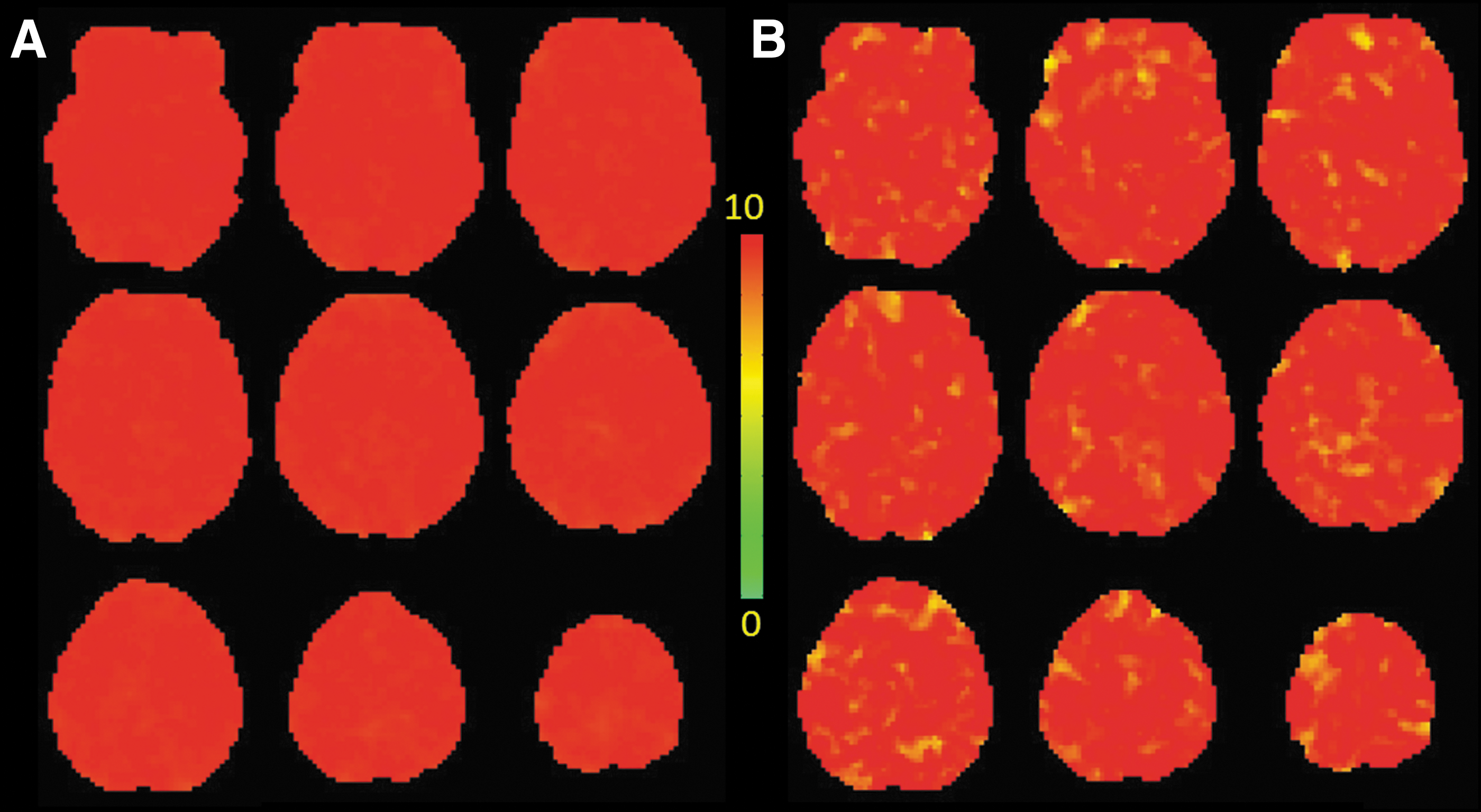
The values in parentheses of Table 2 report the average sACF parameters and FWHM_ap across 21 subjects of the first-level GLM residuals obtained from REST and REST-dtPC datasets. Figures 4 and 5 display the variation of the average (across 21 subjects) local spatial smoothness and sACF a parameter of the first-level residuals across the brain obtained from REST and REST-dtPC_opt null fMRI datasets. The sACF parameter maps of the null rsfMRI datasets were similar to those of the first-level GLM residuals.

FIG. 4.

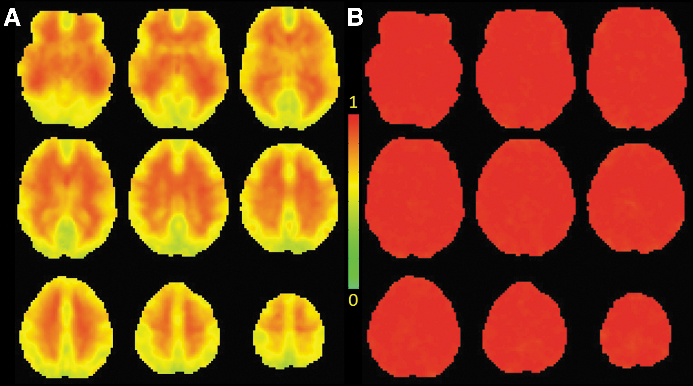
Maps of the group-average local spatial smoothness (FWHM_ap) across the brain of the first-level analysis GLM residuals obtained from (A) REST and (B) REST-dtPC_Opt datasets. Left hemisphere is on the right side of the images.

FIG. 5.

Maps of the group-average local sACF a parameter across the brain of the first-level analysis GLM residuals obtained from (A) REST and (B) REST-dtPC_Opt datasets. Left hemisphere is on the right side of the images.

Effects of PC detrending on cluster-based FWE correction at different CDTs for different null datasets

The top half of Table 3 lists the threshold cluster sizes (obtained through MC simulation via 3dClustSim) needed to judge brain activation at different CDTs significant at specific cluster-based FWE-corrected Type 1 error levels (α-values) based on the sACF parameters of the second-level GLM residuals obtained from analysis of the REST datasets. The values in parentheses show the threshold cluster sizes obtained assuming the sACF to be Gaussian (by setting a = 1; and b = FWHM_ap/2.35482). This table also lists the threshold cluster sizes obtained via the nonparametric permutation test. The results of the same analysis performed on the REST-dtPC_opt dataset are provided in Table 4. Comparing the cluster tables from MC simulations with mixed model sACFs and permutation tests for the REST datasets (in Table 3), it is apparent that cluster-based inferences at CDTs less stringent than p < 0.001 (e.g., 0.01, 0.03, and 0.05) will lead to inordinately large clusters. Further, the threshold cluster sizes for FWE correction obtained with the permutation test were substantially larger than the ones obtained with MC simulation employing Gaussian or mixed-model sACF-based noise approximations, for less stringent CDTs (e.g., for p < 0.01, 0.03, and 0.05). However, the threshold cluster sizes for FWE correction for different CDTs obtained via MC simulation with both mixed- and Gaussian model sACFs fits to the second-level GLM residuals using the REST-dtPC_opt null datasets were very similar to each other and consistently lower than those obtained with the permutation test.

Table 3.

Minimum Cluster Size Thresholds (in Voxels) Needed to Judge BlockA Versus BlockB Group t-Contrast Obtained from the REST Null Dataset with Different Cluster Defining Thresholds Significant at Different Family-Wise Error Rates (α-Values)

CDT, p-value	α <0.05	α <0.03	α <0.01	α <0.001
MC simulation assuming mixed (or Gaussian) model noise
0.05	438 (178)	499 (192)	658 (224)	948 (286)
0.03	240 (116)	274 (126)	369 (147)	569 (191)
0.01	90 (60)	104 (64)	134 (75)	215 (98)
0.001	21 (20)	24 (23)	31 (27)	55 (41)
0.0001	7 (8)	8 (10)	11 (12)	21 (19)
Permutation test
0.05	1378	1960	3573	6761
0.03	612	911	1640	4652
0.01	142	192	386	910
0.001	20	24	40	90
0.0001	5	6	9	18

The top half of the table lists cluster size threshold values obtained with 3dClustSim employing MC simulations employing noise characterized by spatial correlation quantified by the mixed-model sACF parameters estimated from the residuals of second-level BlockA versus BlockB group t-test analysis. The values in the parenthesis denote the cluster size thresholds for the same cell when Gaussian sACF noise with spatial correlation parameterized by FWHM_ap is employed during MC simulation. The bottom half of the table lists equivalent cluster thresholds obtained using permutation tests.

MC, Monte Carlo; sACF, spatial autocorrelation functions.

Table 4.

Minimum Cluster Size Thresholds (in Voxels) Needed to Judge BlockA Versus BlockB Group t-Contrast Obtained from the REST-dtPC_opt Null Dataset with Different Cluster Defining Thresholds Significant at Different Family-Wise Error Rates (α-Values)

CDT, p-value	α <0.05	α <0.03	α <0.01	α <0.001
MC simulation assuming mixed (or Gaussian) model noise
0.05	90 (92)	98 (99)	113 (115)	146 (157)
0.03	60 (61)	64 (65)	74 (75)	102 (99)
0.01	31 (31)	34 (34)	39 (38)	52 (50)
0.001	12 (12)	13 (13)	15 (15)	21 (20)
0.0001	5 (5)	6 (6)	7 (7)	11 (10)
Permutation test
0.05	75	80	94	114
0.03	48	52	61	79
0.01	22	24	27	38
0.001	7	7	8	12
0.0001	3	3	3	5

The top half of the table lists threshold cluster size values obtained with 3dClustSim employing MC simulations employing noise characterized by spatial correlation quantified by the mixed-model sACF parameters estimated from the residuals of second-level BlockA versus BlockB group t-test analysis. The values in the parenthesis denote the cluster size thresholds for the same cells when Gaussian sACF noise with spatial correlation parameterized by FWHM_ap is employed during MC simulation. The bottom half of the table lists equivalent cluster size thresholds obtained using permutation tests.

CDT, cluster defining threshold.

Discussion

Removing nonstochastic signal components from rsfMRI data renders the spatial correlation Gaussian and uniform across the brain

As shown in Figures 2A and 3A, the residuals of the second-level GLM analysis for the simulated block fMRI paradigm, using rsfMRI data as null datasets, exhibited considerable heterogeneity, with gray matter areas exhibiting larger spatial correlation (i.e., higher spatial smoothness and lower values of Gaussianity parameter) than white matter regions. The highest spatial correlation (FWHM_ap) was observed in the default mode network (DMN) and occipital lobe. These results are generally consistent with those reported by other studies (Cox et al., 2017; Eklund et al., 2016).

The first-level GLM residuals as well as the rsfMRI datasets also exhibited similar (although less) heterogeneity in spatial correlation across the brain. The increased spatial correlation and non-Gaussianity in the gray matter areas compared with white matter are likely due to neuronal (i.e., resting-state brain function networks) and other physiological processes. When non-Gaussian signal components from resting-state brain networks, physiological noise, etc. were removed/attenuated by detrending the Eigen time series of the top N_opt PCs from the rsfMRI null datasets, the spatial correlations of the null datasets (REST_dtPC_opt), first- and second-level residuals became nearly Gaussian and almost uniform across the brain (Figs. 2 –6 and Tables 1 and 2).

FIG. 6.

Maps of local spatial smoothness (FWHM_ap) across the brain for (A) first-level residuals (group averaged FWHM_ap), and (B) second-level residuals; obtained from the REST-dtPC_Opt datasets. The spatial smoothness of the second-level residuals is a bit more heterogeneous than that from first-level analysis, but overall similar in magnitude. Left hemisphere is on the right side of the images.

Further, the spatial smoothness of the first- and second-level residuals became similar (Table 2 and Fig. 6) and converged to the intrinsic spatial smoothness of the null datasets (Tables 1 and 2). This shows that if one removes signals from brain function networks and other non-Gaussian signal sources, the spatial structure of the residuals converges to a Gaussian noise field. Finally, comparing the estimated FWHM_ap of the null datasets in Table 1 (obtained through applying FWHM = 5 mm isotropic spatial smoothing to the rsfMRI datasets) with those of Supplementary Table S1 (obtained through applying FWHM = 8 mm smoothing), it is evident that increasing the applied spatial blur by 3 mm resulted in a corresponding 3 mm increase in FWHM_ap of the PC-detrended null datasets that exhibit Gaussian sACF. These results demonstrate that once the non-Gaussian signal components are removed from fMRI data, their spatial smoothness is completely determined by the applied spatial filter.

Removing non-Gaussian signal components from rsfMRI data renders cluster-based FWE-corrected inferences with Gaussian sACF valid

Table 3 shows that when rsfMRI data are used as null datasets, cluster-based FWE-corrected inferences at CDTs less stringent than p < 0.001 (i.e., p < 0.05, 0.03, and 0.01) yield inordinately large threshold clusters sizes. Further MC simulation with simulated noise characterized by both mixed-model and pure Gaussian model parameterizations of the sACF yields much smaller threshold cluster sizes than the nonparametric permutation test, for CDTs less stringent than p < 0.001. Thus, if permutation test-based inferences were to be considered as exact (Eklund et al., 2016), inferences made on the basis of MC simulation with Gaussian or mixed-model approximations of the sACF (Eq. 1) may not be valid for CDTs less stringent than p < 0.001 (e.g., for p < 0.05, 0.03, and 0.01). This is consistent with the results for block paradigms described in Cox et al. (2017).

When null fMRI datasets created by removing non-Gaussian signal components from rsfMRI datasets are employed (Table 4), MC simulation with both mixed-model and Gaussian approximations of the sACFs yields almost identical estimates for threshold cluster sizes for different CDTs and FWE α-values, indicating that the sACF is nearly Gaussian. Further, these MC-based inferences are more conservative than the equivalent permutation test-based nonparametric inferences. However, ideally, CDT p values should be less than the FWE α-values chosen to obtain small enough significant activation clusters for ensuring functional specificity (Woo et al., 2014).

Finally, if one were to compare the Gaussian (matched to empirical FWHM of spatial noise) model sACF results for REST null datasets (Table 3) with the cluster size table results (permutation or mixed model) for REST-dtPC_opt null datasets (Table 4), one can say that if the alternate hypothesis of the prior studies adjudged to have inflated false positives in Eklund et al. (2016) were to be revised to include signals from brain function networks not relevant to the fMRI task under investigation, as well as physiological noise and other non-stochastic signal sources, then the inferences made in these studies based on the assumption of Gaussian and uniform spatial correlation across the brain could be considered still valid.

Methodological considerations

In this study, for each subject, an ideal set of null fMRI datasets (REST-dtPC_opt) was formed by selecting the minimum number of PCs (among 40, 110, 130, 150, and 170) that was required to obtain a PC-detrended dataset that exhibited Gaussian spatial correlation. N_opt varied from 110 to 150, with 17 out 21 subjects exhibiting N_opt = 110. The variation in N_opt across subjects could reflect inter-individual differences in brain function networks, as well as in physiological processes and motion artifacts.

In the method adopted to select N_opt, the sACF of the REST-dtPC_opt dataset was deemed to be Gaussian when the mixed-model sACF Gaussianity parameter a reached its maximum (algorithm constrained) value of 0.9940. Instead of using the AFNI software determined limit (a ≥ 0.9940), which may be based on loss of computational reliability, it may be optimal to use a more conservative Gaussianity criterion for sACF a (e.g., a ≥ 0.99) to determine N_opt. Re-analyzing the data with this criterion for Gaussian sACF yielded N_opt = 110, for 19 out of 21 subjects, and N_opt = 130 and 150 for the remaining two subjects. However, the results for sACF and cluster sizes presented in the figures and tables in this article did not change appreciably. Further, the estimated FWHM_ap of the PC-detrended null datasets exhibiting Gaussian sACF (see Table 1 and Supplementary Table S1) increased roughly by the same amount that the applied spatial blur was increased, demonstrating the validity of the method adopted in this study to determine N_opt. Evolving more formal methods to determine N_opt is left for future studies.

Since the PCA algorithm is intended to arrive at an orthogonal Eigenvector basis where the maximum amount of dataset variance is encoded in the first principal component, and the amount of dataset variance explained progressively decreases from the first PC to the last, the PCs will not be independent when the dataset has a number of non-Gaussian signal sources. This will result in independent signal sources (e.g., different brain networks, physiological signals, motion artifacts, etc.) being mixed within the PCs. However, even with these constraints, one could discern different brain networks (e.g., DMN) and physiological signals in the PCs, as shown in Supplementary Figure S1 for a representative subject. This indicates that the PC-detrending procedure, indeed, maximizes the attenuation of non-Gaussian signal components in the null fMRI datasets. A separate analysis employing ICA (with varying dimensions) instead of PCA revealed similar results (results not shown). However, the number of ICs needed to account for all non-Gaussian signals was greater than N_opt.

Finally, an implicit assumption employed in this proof-of-concept exercise is that one can (if needed) separate signals due to brain activation related to a given task fMRI paradigm, from signals related to other brain network activity, physiological processes, etc., under the GLM framework. The companion article (Gopinath et al., 2017) discusses this issue along with providing a potential solution for obtaining first-level GLM residuals with nearly uniform and Gaussian sACF across the brain.

Conclusion

In this study, we demonstrated that removing non-Gaussian signal sources from the rsfMRI data yields null fMRI datasets with nearly uniform and Gaussian spatial correlation across the brain. GLM analysis on simulated fMRI paradigms using PC-detrended null fMRI datasets yields first- and second-level residuals with uniform and Gaussian sACFs. Cluster-based FWE-corrected inferences obtained with MC simulations employing noise characterized by Gaussian sACF parameters of the second-level analysis GLM residuals yield more conservative FWE estimates than nonparametric permutation tests, indicating validity of inferences based on Gaussian spatial noise models.

Footnotes

Acknowledgments

This study was supported by the Department of Radiology and Imaging Sciences, Emory University. Support to K.S. from the Atlanta VAMC is also gratefully acknowledged.

Author Disclosure Statement

No competing financial interests exist.

References

Birn

, Diamond

, Smith

, Bandettini

. 2006. Separating respiratory-variation-related fluctuations from neuronal-activity-related fluctuations in fMRI. Neuroimage, 31:1536–1548.

Buckner

, Sepulcre

, Talukdar

, Krienen

, Liu

, Hedden

, et al. 2009. Cortical hubs revealed by intrinsic functional connectivity: mapping, assessment of stability, and relation to Alzheimer's disease. J Neurosci, 29:1860–1873.

Buxton

RB.

2009. Introduction to Functional Magnetic Resonance Imaging: Principles and Techniques, 2nd ed. New York: Cambridge University Press.

Carmack

, Spence

, Schucany

, Gunst

, Lin

, Haley

. 2012. A new class of semiparametric semivariogram and nugget estimators. Comput Stat Data Anal, 56:1737–1747.

Chang

, Cunningham

, Glover

. 2009. Influence of heart rate on the BOLD signal: the cardiac response function. Neuroimage, 44:857–869.

Cox

RW.

1996. AFNI: software for analysis and visualization of functional magnetic resonance neuroimages. Comput Biomed Res, 29:162–173.

Cox

, Chen

, Glen

, Reynolds

, Taylor

. 2017. FMRI clustering in AFNI: false positive rates redux. Brain Connect, 7:152–171.

Dagli

, Ingeholm

, Haxby

. 1999. Localization of cardiac-induced signal change in fMRI. Neuroimage, 9:407–415.

Eklund

, Nichols

, Knutsson

. 2016. Cluster failure: why fMRI inferences for spatial extent have inflated false-positive rates. Proc Natl Acad Sci U S A, 113:7900–7905.

10.

Forman

, Cohen

, Fitzgerald

, Eddy

, Mintun

, Noll

. 1995. Improved assessment of significant activation in functional magnetic resonance imaging (fMRI): use of a cluster-size threshold. Magn Reson Med, 33:636–647.

11.

Glover

, Li

, Ress

. 2000. Image-based method for retrospective correction of physiological motion effects in fMRI: RETROICOR. Magn Reson Med, 44:162–167.

12.

Gopinath

, Gandhi

, Goyal

, Jiang

, Fang

, Ouyang

, et al. 2012. FMRI reveals abnormal central processing of sensory and pain stimuli in ill Gulf War veterans. Neurotoxicology, 33:261–271.

13.

Gopinath

, Krishnamurthy

, Lacey

, Sathian

. 2017. Accounting for non-Gaussian sources of spatial correlation in parametric fMRI paradigms II: a method to obtain first level analysis residuals with uniform and Gaussian spatial autocorrelation function and independent and identically distributed time-series. Brain Connect [Epub ahead of print] DOI: 10.1089/brain.2017.0522

14.

Gopinath

, Ringe

, Goyal

, Carter

, Dinse

, Haley

, Briggs

. 2011. Striatal functional connectivity networks are modulated by fMRI resting state conditions. Neuroimage, 54:380–388.

15.

Kiebel

, Poline

, Friston

, Holmes

, Worsley

. 1999. Robust smoothness estimation in statistical parametric maps using standardized residuals from the general linear model. Neuroimage, 10:756–766.

16.

Kriegeskorte

, Bodurka

, Bandettini

. 2008. Artifactual time-tourse correlations in echo-planar fMRI with implications for studies of brain function. Int J Imaging Syst Technol, 18:345–349.

17.

Lebois

, Papies

, Gopinath

, Cabanban

, Quigley

, Krishnamurthy

, et al. 2015. A shift in perspective: decentering through mindful attention to imagined stressful events. Neuropsychologia, 75:505–524.

18.

Liau

, Perthen

, Liu

. 2008. Caffeine reduces the activation extent and contrast-to-noise ratio of the functional cerebral blood flow response but not the BOLD response. Neuroimage, 42:296–305.

19.

McGregor

, Sudhyadhom

, Nocera

, Seff

, Crosson

, Butler

. 2015. Reliability of negative BOLD in ipsilateral sensorimotor areas during unimanual task activity. Brain Imaging Behav, 9:245–254.

20.

Moffett

, Crosson

, Spence

, Case

, Levy

, Gopinath

, et al. 2015. Word-finding impairment in veterans of the 1991 Persian Gulf War. Brain Cogn, 98:65–73.

21.

Nehlig

, Boyet

. 2000. Dose-response study of caffeine effects on cerebral functional activity with a specific focus on dependence. Brain Res, 858:71–77.

22.

Pruim

, Mennes

, van Rooij

, Llera

, Buitelaar

, Beckmann

. 2015. ICA-AROMA: a robust ICA-based strategy for removing motion artifacts from fMRI data. Neuroimage, 112:267–277.

23.

Rack-Gomer

, Liau

, Liu

. 2009. Caffeine reduces resting-state BOLD functional connectivity in the motor cortex. Neuroimage, 46:56–63.

24.

Salimi-Khorshidi

, Douaud

, Beckmann

, Glasser

, Griffanti

, Smith

. 2014. Automatic denoising of functional MRI data: combining independent component analysis and hierarchical fusion of classifiers. Neuroimage, 90:449–468.

25.

Sathian

, Lacey

, Stilla

, Gibson

, Deshpande

, Hu

, et al. 2011. Dual pathways for haptic and visual perception of spatial and texture information. Neuroimage, 57:462–475.

26.

Smith

, Fox

, Miller

, Glahn

, Fox

, Mackay

, et al. 2009. Correspondence of the brain's functional architecture during activation and rest. Proc Natl Acad Sci U S A, 106:13040–13045.

27.

Smith

, Jenkinson

, Woolrich

, Beckmann

, Behrens

, Johansen-Berg

, et al. 2004. Advances in functional and structural MR image analysis and implementation as FSL. Neuroimage 23 Suppl, 1:S208–S219.

28.

Thesen

, Heid

, Mueller

, Schad

. 2000. Prospective acquisition correction for head motion with image-based tracking for real-time fMRI. Magn Reson Med, 44:457–465.

29.

Van Dijk

, Hedden

, Venkataraman

, Evans

, Lazar

, Buckner

. 2010. Intrinsic functional connectivity as a tool for human connectomics: theory, properties, and optimization. J Neurophysiol, 103:297–321.

30.

Weisskoff

R.M.

, 1996. Simple measurement of scanner stability for functional NMR imaging of activation in the brain. Magn Reson Med, 36:643–645.

31.

Woo

, Krishnan

, Wager

TD.

, 2014. Cluster-extent based thresholding in fMRI analyses: pitfalls and recommendations. Neuroimage, 91:412–419.

Supplementary Material

Please find the following supplemental material available below.

For Open Access articles published under a Creative Commons License, all supplemental material carries the same license as the article it is associated with.

For non-Open Access articles published, all supplemental material carries a non-exclusive license, and permission requests for re-use of supplemental material or any part of supplemental material shall be sent directly to the copyright owner as specified in the copyright notice associated with the article.

0.00 MB

0.22 MB