Accounting for Non-Gaussian Sources of Spatial Correlation in Parametric Functional Magnetic Resonance Imaging Paradigms II: A Method to Obtain First-Level Analysis Residuals with Uniform and Gaussian Spatial Autocorrelation Function and Independent and Identically Distributed Time-Series

Abstract

In a recent study Eklund et al. have shown that cluster-wise family-wise error (FWE) rate-corrected inferences made in parametric statistical method-based functional magnetic resonance imaging (fMRI) studies over the past couple of decades may have been invalid, particularly for cluster defining thresholds less stringent than p < 0.001; principally because the spatial autocorrelation functions (sACFs) of fMRI data had been modeled incorrectly to follow a Gaussian form, whereas empirical data suggest otherwise. Hence, the residuals from general linear model (GLM)-based fMRI activation estimates in these studies may not have possessed a homogenously Gaussian sACF. Here we propose a method based on the assumption that heterogeneity and non-Gaussianity of the sACF of the first-level GLM analysis residuals, as well as temporal autocorrelations in the first-level voxel residual time-series, are caused by unmodeled MRI signal from neuronal and physiological processes as well as motion and other artifacts, which can be approximated by appropriate decompositions of the first-level residuals with principal component analysis (PCA), and removed. We show that application of this method yields GLM residuals with significantly reduced spatial correlation, nearly Gaussian sACF and uniform spatial smoothness across the brain, thereby allowing valid cluster-based FWE-corrected inferences based on assumption of Gaussian spatial noise. We further show that application of this method renders the voxel time-series of first-level GLM residuals independent, and identically distributed across time (which is a necessary condition for appropriate voxel-level GLM inference), without having to fit ad hoc stochastic colored noise models. Furthermore, the detection power of individual subject brain activation analysis is enhanced. This method will be especially useful for case studies, which rely on first-level GLM analysis inferences.

Introduction

Blood oxygenation level-dependent (BOLD) functional magnetic resonance imaging (fMRI) has been the pre-eminent technique to study brain function and pathology over the last two decades (Buxton, 2009; Crosson et al., 2007). A preponderance of fMRI studies on brain function over this period have adopted parametric statistical methods under the general linear model (GLM) framework to assess brain activation.

Recently, the validity of cluster-based family-wise error (FWE)-corrected inferences made in many of these studies has been called into question by Eklund and associates (2016), who stated that the main source of these incorrect inferences was that the spatial autocorrelation function (sACF) of the fMRI data had been assumed to be Gaussian and uniform across the brain, whereas empirical data suggest otherwise (Carmack et al., 2012; Eklund et al., 2016). This is reflected in the residuals of the GLM analysis possessing considerable heterogeneity in smoothness across the brain, as well as non-Gaussian sACFs.

In Part 1 of this study presented in the companion article (Gopinath et al., 2017) based on Eklund and associates (2016) and Cox and associates (2017), we used resting-state fMRI (rsfMRI) as null data sets to show that removing non-Gaussian signal arising from brain function networks, physiological processes, motion artifacts, and so on from null fMRI data sets renders the spatial correlation in these data sets, as well as first- and second-level residuals from GLM analysis conducted on these null data sets, uniform and Gaussian across the brain.

In Part 2 of this study presented here, we use the knowledge gained from the results of Part 1 to introduce a method for block fMRI paradigms to obtain first-level analysis GLM residuals with nearly uniform and Gaussian sACFs across the brain, based on quantification and orthogonalization of signal from non-Gaussian sources such as coherent activity in brain function networks, physiological processes, and motion, and other image acquisition artifacts, during first-level GLM analysis.

Furthermore, we show that this procedure renders the first-level GLM analysis voxel time-series residuals obtained with ordinary least squares (OLS) multiple linear regression, independent and identically distributed (IID), which is a necessary condition for obtaining valid first-level analysis voxel-level inferences, without having to fit ad hoc stochastic colored noise models. Accounting for non-Gaussian and nonstochastic signal components in the residuals will, in addition to making the GLM voxel time-series residuals IID, reduce their variance and hence increase the detection power of first-level GLM analyses. This will be especially beneficial to case studies (Crosson et al., 2005; Katz et al., 2012).

Furthermore, ensuring uniform and Gaussian sACF of first-level residuals will permit the use of parametric cluster-based FWE correction methods to assess the significance of individual subject brain activation and contrast maps, which are preferable to nonparametric permutation tests for complex fMRI paradigms used in many studies.

The basis for this proposed method is that it is well known that the residuals of GLM-based fMRI first-level analysis exhibit coherent activity in brain function networks nearly analogous to rsfMRI data (Fair et al., 2007; Turk-Browne, 2013). Relatedly, the brain areas that exhibit strongest temporal (Sahib et al., 2016) and spatial correlation (Eklund et al., 2016) coincide with what are considered hubs of functional connectivity networks, for example, posterior cingulate cortex (Buckner et al., 2009). Further physiological processes, such as cardiac (Chang et al., 2009; Dagli et al., 1999; Glover et al., 2000) and respiration (Birn et al., 2006; Glover et al., 2000) fluctuations, and motion artifacts (Power et al., 2012) can introduce both temporal and spatial correlation on fMRI time-series and first-level residuals if not adequately modeled.

Currently, temporal (serial) correlation in fMRI GLM residuals is handled by fitting the fMRI time-series to autoregressive (AR) (Bullmore et al., 1996; Friston et al., 2002) plus white noise, or autoregressive moving average (ARMA) (Cox et al., 2017) models. However, these approaches essentially end up fitting stochastic models to deterministic brain signals. Hence, the order and degree of AR and moving average (MA) parameters will depend on the temporal resolution of the fMRI data (Purdon et al., 2001; Sahib et al., 2016). Furthermore, AR and MA order and parameters will ideally need to be fitted separately for all voxels in the brain (Purdon et al., 2001; Sahib et al., 2016) to account for heterogeneity in temporal correlation across the brain induced by different processes mentioned above.

Furthermore, these methods of accounting for temporal correlation do not take into account the common sources of temporal and spatial correlation in fMRI data. However, if the different nonstochastic signals arising from unmodeled brain function networks, physiological noise, and so on, introducing spatial and temporal correlation in the GLM residuals, are quantified with the principal component analysis (PCA) and removed, one could obtain IID first-level analysis GLM residuals with Gaussian spatial correlation, without having to fit ad hoc stochastic models to fMRI time-series data.

The main assumptions inherent in the proposed method are as follows: (1) the intrinsic spatial correlation in fMRI data in the absence of quantifiable signal related to brain function, physiological responses, and subject motion is Gaussian; (2) in the absence of the above-mentioned nonstochastic signal components, the fMRI voxel time-series (after accounting for MRI scanner-related drifts and attainment of steady state of longitudinal magnetization) is IID in time, that is, the spatial and temporal correlation of fMRI time-series data arises from similar sources; and (3) quantifying and removing nonstochastic signal components from the first-level analysis GLM residuals will, in addition to rendering the spatial correlation of the residuals Gaussian, also render the residuals voxel-time series IID in time, which is a necessary condition for obtaining valid GLM inference.

A potential cost incurred in this method is that the GLM regression parameters expressing brain activation (e.g., amplitude of BOLD response to various stimulus types) are estimated with OLS-based multiple linear regression, without accounting for temporal correlations introduced by different nonstochastic brain signals mentioned above. Hence, the brain activation parameters will, in general, be slightly overestimated or underestimated. However, the benefits of comprehensively accounting for spatial and temporal correlation in the residuals, as described below, justify the cost of slightly suboptimal activation amplitude estimation.

Materials and Methods

Participants

Twenty-one right-handed participants were recruited from the Atlanta metropolitan area (11 males and 10 females; median age = 22 years). Exclusion criteria for the study were as follows: pregnancy, metallic implants or other contraindications to MRI; history of psychiatric illness or substance abuse or dependence; significant family history of psychiatric or neurological illness; current use of any centrally acting medications; and serious medical or neurological illness. Since caffeine can alter neural firing (Fredholm et al., 1999; Nehlig, 1999; Nehlig and Boyet, 2000) as well as fMRI BOLD responses (Behzadi and Liu, 2006; Liau et al., 2008; Liu et al., 2004), participants were asked to refrain from ingesting caffeine products for 12 h before the scan. Written informed consent was obtained from participants under an IRB-approved protocol.

Experimental design

Four visual processing fMRI scans were acquired from each subject. The fMRI stimulus paradigm for each scan comprised three blocks each of five types of stimuli: faces, objects, nature scenes, body parts, and scrambled objects (a low-level control). Each block of a given type (e.g., faces) of stimuli was 12-sec long, with six black and white photographs of that type (e.g., faces) each presented for 1-sec duration, with intervening 1-sec blocks during which the screen was blank. The participants were asked to press a button each time a picture was repeated consecutively within a block to ensure the participants paid attention to all the stimuli. There was an average of one repeated picture presentation within each block.

Each stimulus block was followed by a fixation block (white cross on a black background) lasting 12, 14, or 16 sec (sampled from a uniform random distribution of interblock intervals). The order of presentation of the five block types was randomized. A 14-sec fixation period at the beginning of each fMRI run was used to acclimatize the participant to the echo-planar imaging (EPI) scan, as well as to obtain baseline parameters for the GLM. Stimuli were presented by means of a high-resolution liquid crystal display projection system (1400 × 1050 SXGA, 4200 lumens, 1300:1 contrast ratio) delivered from the back of the suite onto a custom-fit screen mounted within the scanner bore behind the participant's head. Stimulus presentation was controlled by Presentation™ (Albany, CA) software.

Image acquisition

MRI was acquired on a 3T Siemens TIM Trio scanner with a 12-channel receiver array head coil. BOLD fMRI scans were acquired with a gradient echo EPI sequence, with repetition time (TR)/echo time (TE) = 2000/25 msec and flip angle (FA) = 90°; 42 sagittal slices (3.5 mm thick; in-plane resolution 3 mm × 3 mm) covering the whole brain; 210 scan volumes. Prospective real-time motion correction (Thesen et al., 2000) was used with all EPI scans to minimize motion artifacts. Also, a whole-brain three-dimensional (3D) T1-weighted MPRAGE sequence (FOV = 230 mm; TR/TI/TE/FA = 2250/900/3 msec/9°; 0.9 × 0.9 × 1 mm resolution; TI = inversion time) was acquired to provide anatomic detail. All these scans were acquired with parallel imaging: GRAPPA acceleration factor = 2; 24 (36 for MPRAGE) phase-encoding reference lines. Foam padding was provided to minimize head motion.

Data analysis

Only the data from the first visual processing fMRI scan are presented in this proof-of-concept study.

Preprocessing

Data analysis was performed using the analysis of functional neuroimages (AFNI) (Cox, 1996) and FMRIB software library (FSL) (Smith et al., 2004) software packages and in-house programs written in MATLAB (MathWorks, Natick, MA). The fMRI voxel time-series were temporally shifted to account for differences in slice acquisition times, 3D volume registered to a base volume to account for global rigid motion, coregistered to the T1-weighted high-resolution anatomic scan, spatially normalized to the MNI152 template, and resampled to 3 × 3 × 3 mm voxel resolution. The fMRI data were then spatially smoothed with a full-width at half-maximum (FWHM) of 5 mm isotropic Gaussian kernel. For each stimulus type, a 203 time point stimulus vector was constructed (after ignoring first four volumes to ensure that the magnetization reached steady state, as well as the last three volumes to eliminate truncation artifacts introduced by the time-shifting program).

First-level analysis

For each voxel, the signal was modeled as the sum of the convolutions of the five stimulus vectors with a one free parameter (amplitude) gamma variate function, plus third-order polynomial drifts and constant baseline, with a GLM under the multiple linear regression-based framework with OLS approach. The t-statistic maps of the GLM estimate regression coefficients for amplitudes of each category (e.g., Body) and the t-statistic contrast (e.g., Body-Object) maps expressed the significance of activation for that category and contrast, respectively, for each subject. The OLS approach was adopted for multiple linear regression analysis, to apply the PCA-based method described below.

For comparison with a current standard practice of modeling temporal correlation, the above multiple regression analysis was repeated with the generalized least squares (GLS) approach with ARMA(1,1) prewhitening to account for temporal correlation (using AFNI programs 3dDeconvolve and 3dREMLfit).

PCA-based decomposition of first-level residuals

The aim of this proof-of-concept study was to put forward a method to obtain first-level analysis GLM residuals with uniform and Gaussian sACFs across the brain, which also renders the GLM residuals IID in time. This could be accomplished by characterizing (with PCA) and removing (with multiple linear regression) signal from non-Gaussian (neural, physiological, or artifactual) sources from the residuals. To this end, the four-dimensional first-level residuals time-series data sets (RSDL) obtained using OLS multiple linear regression described above were decomposed with PCA using the 3dpc program in the AFNI software suite (Cox, 1996) into N 3D spatial principal components (PCs) along with N orthogonal one-dimensional (1D) PC eigen-time-series, ranked from the highest to lowest eigenvalue, where N is the length of the fMRI time-series.

First-level GLM analysis with PC orthogonalization

Following this step, the first-level GLM analysis was repeated (using OLS) with simultaneous orthogonalization (in separate analyses) of the top 40, 70, 80, 100, and 133 PC 1D eigen-time-series, which roughly corresponded to accounting for 60%, 70%, 75%, 80%, and 90%, respectively, of the net variance in each RSDL data set to get an idea of the optimal number of PCs (N _opt) needed to render the estimated sACF (Estimation of spatial correlation section) nearly uniform and Gaussian across the brain while keeping the reduction of degrees of freedom involved in PC orthogonalization to a minimum. The PC-orthogonalized GLM essentially removes signal proportional to the PC eigen-time-series from the residuals.

The inherent assumption in this method is that the spatial and temporal correlations in fMRI data arise from similar nonstochastic sources. Hence, it is expected that the optimal PC-orthogonalized GLM residuals (RSDL-ortN_optPC) will be IID in time, which is a necessary condition for obtaining valid first-level analysis inferences, without having to fit ad hoc stochastic colored noise models. The normality of the resultant RSDL-ortN_optPC voxel time-series was assessed with Anderson–Darling tests (Stephens, 1974) using the 3dNormalityTest program in AFNI. The normality of the conventional multiple linear regression residuals obtained through the OLS approach (RSDL) and the whitened residuals obtained with the GLS approach (RSDL_GLS) was also tested in the same manner.

This PC orthogonalization procedure, while decreasing unmodeled variance in the resultant residuals (RSDL-ortN_optPC), should not affect the activation amplitude regression coefficient estimates since the residuals are orthogonal to the space of the regressors. Hence, this method will increase the significance of activation of individual subject activation maps, in addition to rendering the RSDL-ortN_optPC data set voxel time-series nearly IID, and the spatial correlation of RSDL-ortN_optPC data sets more uniform and Gaussian. The second-level analysis results should not be affected by this method.

Individual subject activation maps

To examine the effects of the PC orthogonalization procedure on the individual subject activation maps for different visual stimulus categories as well as between-category contrast maps, the t-statistics of corresponding to the GLM-estimate amplitudes and contrasts were converted to z-scores to account for the different degrees of freedom of the RSDL (as well as RSDL_GLS) and the PC-orthogonalized RSDL-ortN_optPC data sets.

Multiple comparison corrected inference

Statistical inference test maps were clustered, and the significance of activations, accounting for multiple comparisons, was derived by means of Monte Carlo (MC) simulation of the process of image generation, estimated spatial correlation (see Estimation of spatial correlation section) of voxels, intensity thresholding, masking (whole brain), and cluster identification (Cox et al., 2017) through the 3dClustSim program implemented in AFNI. In this study, two voxels were assumed to belong to a cluster for a given cluster detection threshold (CDT) (p-value threshold for all voxels in the cluster) if and only if they both exhibited activation stronger than the CDT and faces of the cubic voxels touched each other.

The CDT was varied over a number of prespecified values between p < 0.05 and p < 0.001, and the minimum cluster size needed to judge the cluster-level activation significant at different prespecified FWE rates (α values) was computed. The spatial correlation among voxels in the random noise fields used during MC simulations was quantified by the whole-brain sACF parameters (see Estimation of spatial correlation section) estimated from the RSDL, RSDL_GLS, and RSDL-ortN_optPC data sets for the corresponding subjects for inferences based on the conventional GLM with OLS and GLS methods, and the optimal PC-orthogonalized GLM analysis method, respectively.

Estimation of spatial correlation

The sACF for all data sets was estimated at both the whole-brain level and within 25-mm-radius spherical local neighborhoods across the brain using the 3dFWHMx program in AFNI, which expresses sACF as a mixed Gaussian+monoexponential model, to account for longer tails in the shape of the empirical sACFs seen in fMRI data than a pure squared-exponential model can accommodate (Cox et al., 2017). \documentclass{aastex}\usepackage{amsbsy}\usepackage{amsfonts}\usepackage{amssymb}\usepackage{bm}\usepackage{mathrsfs}\usepackage{pifont}\usepackage{stmaryrd}\usepackage{textcomp}\usepackage{portland, xspace}\usepackage{amsmath, amsxtra}\usepackage{upgreek}\pagestyle{empty}\DeclareMathSizes{10}{9}{7}{6}\begin{document} \begin{align*} sACF = a \times \exp \left( { - { \frac { { r^2 } } { 2 { b^2 } } } } \right) + \left( { 1 - a } \right) \times \exp \left( { - \frac { r } { c } } \right) , \tag { 1 } \end{align*} \end{document}

where r is the radius and a is the parameter that expresses the mixture of Gaussian and monoexponential portions of the sACF. The parameter \documentclass{aastex}\usepackage{amsbsy}\usepackage{amsfonts}\usepackage{amssymb}\usepackage{bm}\usepackage{mathrsfs}\usepackage{pifont}\usepackage{stmaryrd}\usepackage{textcomp}\usepackage{portland, xspace}\usepackage{amsmath, amsxtra}\usepackage{upgreek}\pagestyle{empty}\DeclareMathSizes{10}{9}{7}{6}\begin{document}$$a \in$$ \end{document} (0, 1), but is constrained to vary between 0.06 and 0.9940 by the nonlinear optimization algorithm used to estimate the spatial correlation of the data. A high value of a will indicate that sACF was nearly Gaussian. The parameters b and c together quantify the spatial smoothness of the data and are constrained to be positive (b, c > 0) and reflect the smoothness of the Gaussian and monoexponential components of the sACF, respectively. Furthermore, the apparent FWHM (FWHM_ap) of the empirical sACF was calculated for all data sets (both at the whole-brain level and within spherical local neighborhoods of 25 mm).

Results

All subjects exhibited category-specific brain activation to body-part, face, scene, and object stimuli as expected from previous studies (Bracci et al., 2010; Epstein and Higgins, 2007; Kanwisher et al., 1997; Malach et al., 1995). These category-specific activations obtained from this study have been reported elsewhere (Gopinath et al., 2013).

Table 1 lists the average sACF parameters (across the group) of the residuals of conventional GLM (RSDL and the whitened RSDL_GLS) as well as GLM with different levels of PC orthogonalization (e.g., RSDL-ort80PC). The sACF a parameter that quantifies the Gaussian part of the mixed noise sACF model reached its maximum value of 0.994 (up to three significant figures) for all subjects when component time-series corresponding to the top 80 PCs or higher were simultaneously orthogonalized during the GLM analysis. This indicates that the sACFs of the residuals data sets were approximately Gaussian after the first 80 PCs (N _opt = 80) were regressed out.

Table 1.

The Estimated sACF Parameters (Assuming Mixed Model sACF) and the Empirical Spatial Smoothness (FWHM_ap) for the First-Level GLM Analysis Residuals Using the OLS Approach (RSDL) and the GLS Approach (RSDL_GLS), and the Residuals Obtained Using GLM Analysis with Simultaneous PC Orthogonalization (Mean Across 21 Subjects ± Standard Deviation)

Residuals	ACF a	ACF b	ACF c	FWHM_gaus
RSDL	0.7015 ± 0.175	4.190 ± 0.060	13.445 ± 0.049	10.91 ± 0.38
RSDL_GLS	0.7646 ± 0.060	4.003 ± 0.073	12.391 ± 1.106	10.13 ± 0.23
RSDL-ort 40PC	0.9692 ± 0.017	3.989 ± 0.057	9.890 ± 2.076	9.44 ± 0.13
RSDL-ort 70PC	0.9939 ± 0.003	3.908 ± 0.053	4.931 ± 4.222	9.19 ± 0.12
RSDL-ort 80PC	0.9940 ± 0.000	3.880 ± 0.050	3.521 ± 1.822	9.12 ± 012
RSDL-ort 100PC	0.9940 ± 0.000	3.835 ± 0.048	2.796 ± 0.202	9.01 ± 0.11
RSDL-ort 133PC	0.9940 ± 0.000	3.808 ± 0.046	2.818 ± 0.161	8.95 ± 0.11

FWHM, full-width at half-maximum; GLM, general linear model; GLS, generalized least squares; OLS, ordinary least squares; PC, principal component; sACF, spatial autocorrelation function.

Effects of PC orthogonalization on the normality of first-level residuals time-series

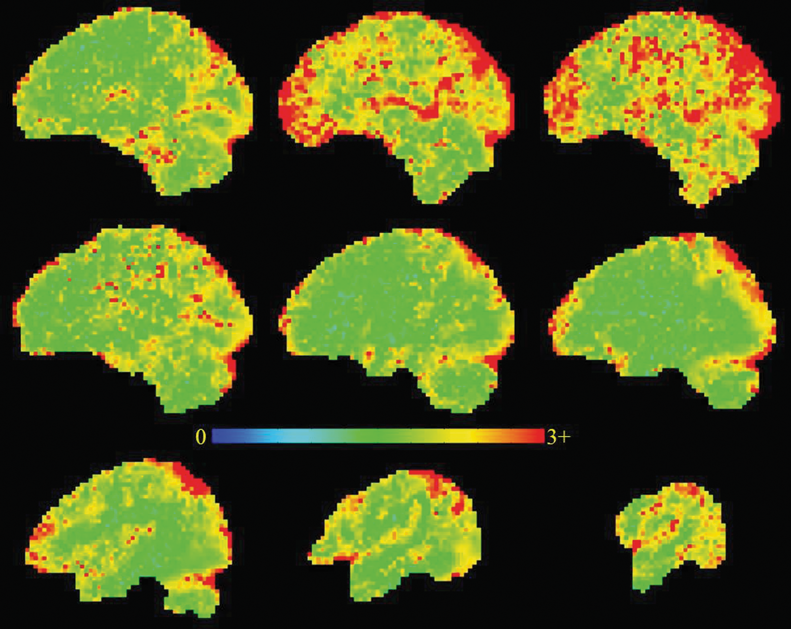
Figure 1A shows the map of Anderson–Darling (AD) test statistics for normality (obtained through application of AFNI's 3dNormalityTest program) for the voxel time-series of the ARMA(1,1)-whitened RSDL_GLS data set for one of the subjects. Figure 1B and C shows the AD statistic maps of the same subject's RSDL-ort80PC and RSDL data sets, respectively. Voxel time-series with AD statistic values greater than 0.787 (corresponding to colors bright yellow to red in the maps) are considered to depart from normality at p < 0.05 (Stephens, 1974).

FIG. 1.

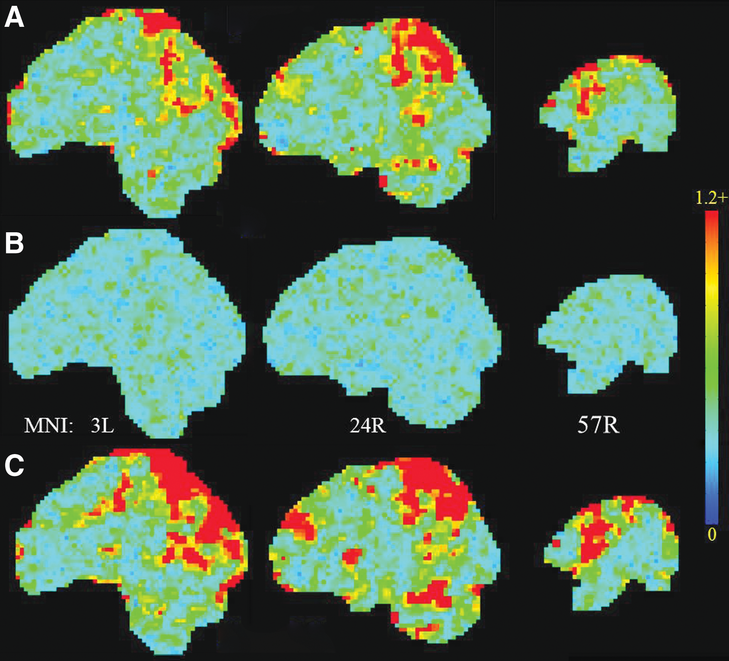
Anderson–Darling statistics maps assessing departures of residuals voxel time-series from normality in the RSDL_GLS (A), RSDL-ort80PC (B), and RSDL (C) data sets.

Using clustering criteria of p < 0.05 and cluster size ≥20 voxels to eliminate isolated voxels, all the subjects' RSDL_GLS data sets showed clusters of voxel time-series exhibiting significant (voxel p < 0.05) departure from normality, that is, failing the IID requirement for valid GLM inference. These voxels, in general, tended to concentrate on brain regions displaying relatively large variance in the residuals time-series. The percentage of RSDL_GLS data set voxel time-series exhibiting significant departure from normality ranged from 0.25% to 22% (with a median of 1.1%). The RSDL data sets exhibited a significantly higher percentage of voxel time-series exhibiting departure from normality compared with RSDL_GLS data sets as expected, ranging from 1% to 28% (with a median of 3.5%).

On the contrary, none of the RSDL-ort80PC data sets showed voxel time-series departing from normality using the same criteria. Thus, the PC orthogonalization procedure rendered the voxel residuals time-series IID for all subjects, and is superior to the standard method of whitening residuals time-series with stochastic colored noise models.

Effects of PC orthogonalization on spatial correlation of first-level residuals

The RSDL_GLS data sets (generated from conventional GLM analysis with GLS approach) exhibited significant spatial correlation, with non-Gaussian ACF as expected, based on previous studies (Eklund et al., 2016). The spatial smoothness, local FWHM_ap (Fig. 2A), and local sACF Gaussianity parameter a (Fig. 3A) of the RSDL_GLS data set also exhibited significant heterogeneity across the brain with gray matter areas exhibiting large local FWHM_ap (and small a parameter) values. The RSDL data sets derived with OLS regression exhibited (not shown) greater heterogeneity in sACF parameters across the brain than the RSDL_GLS data sets. The PC orthogonalization procedure resulted in residuals (RSDL-ort80PC) with much reduced spatial correlation and nearly uniform and Gaussian sACF across the brain (Table 1 and Figs. 2B and 3B).

FIG. 2.

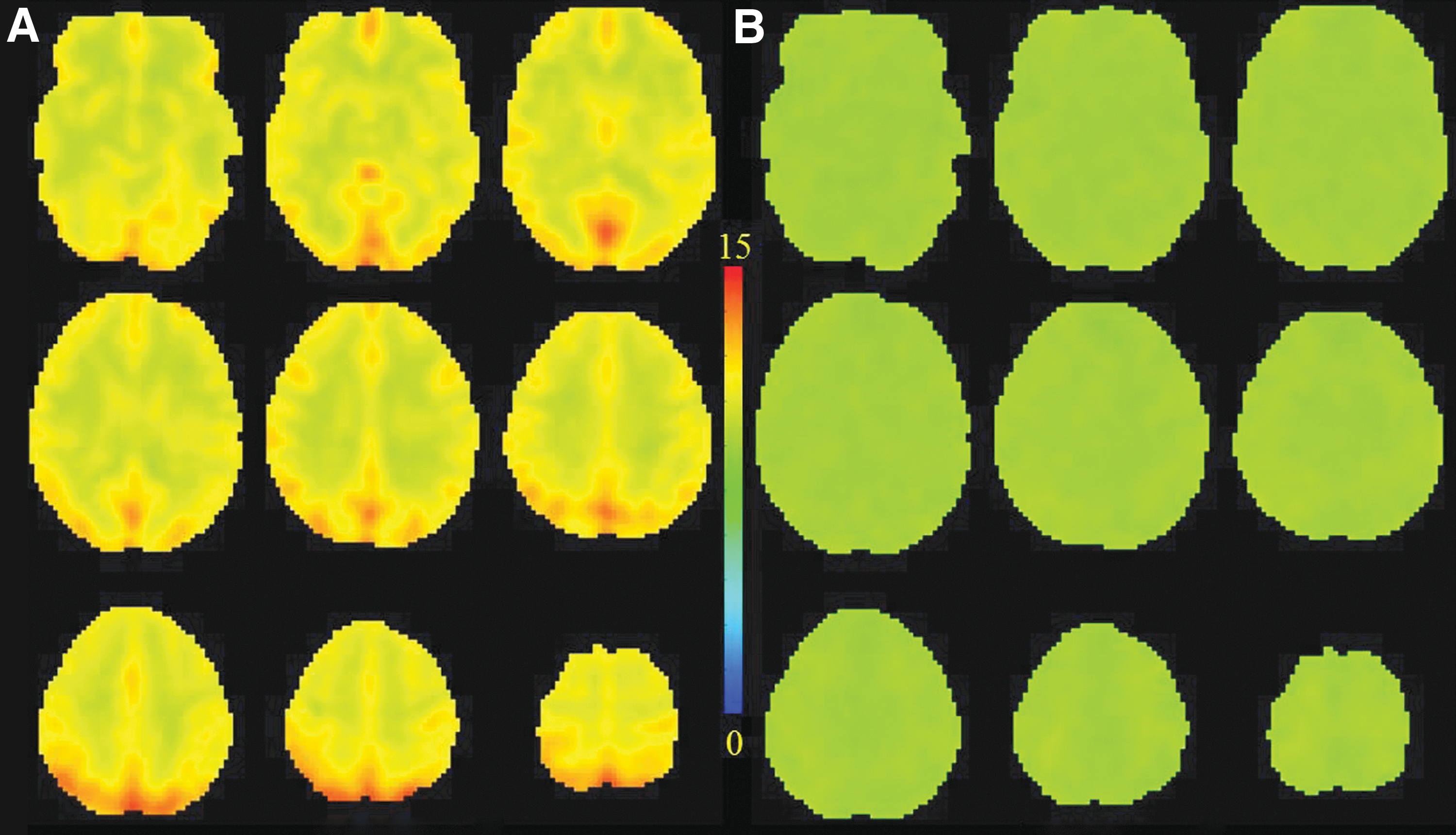
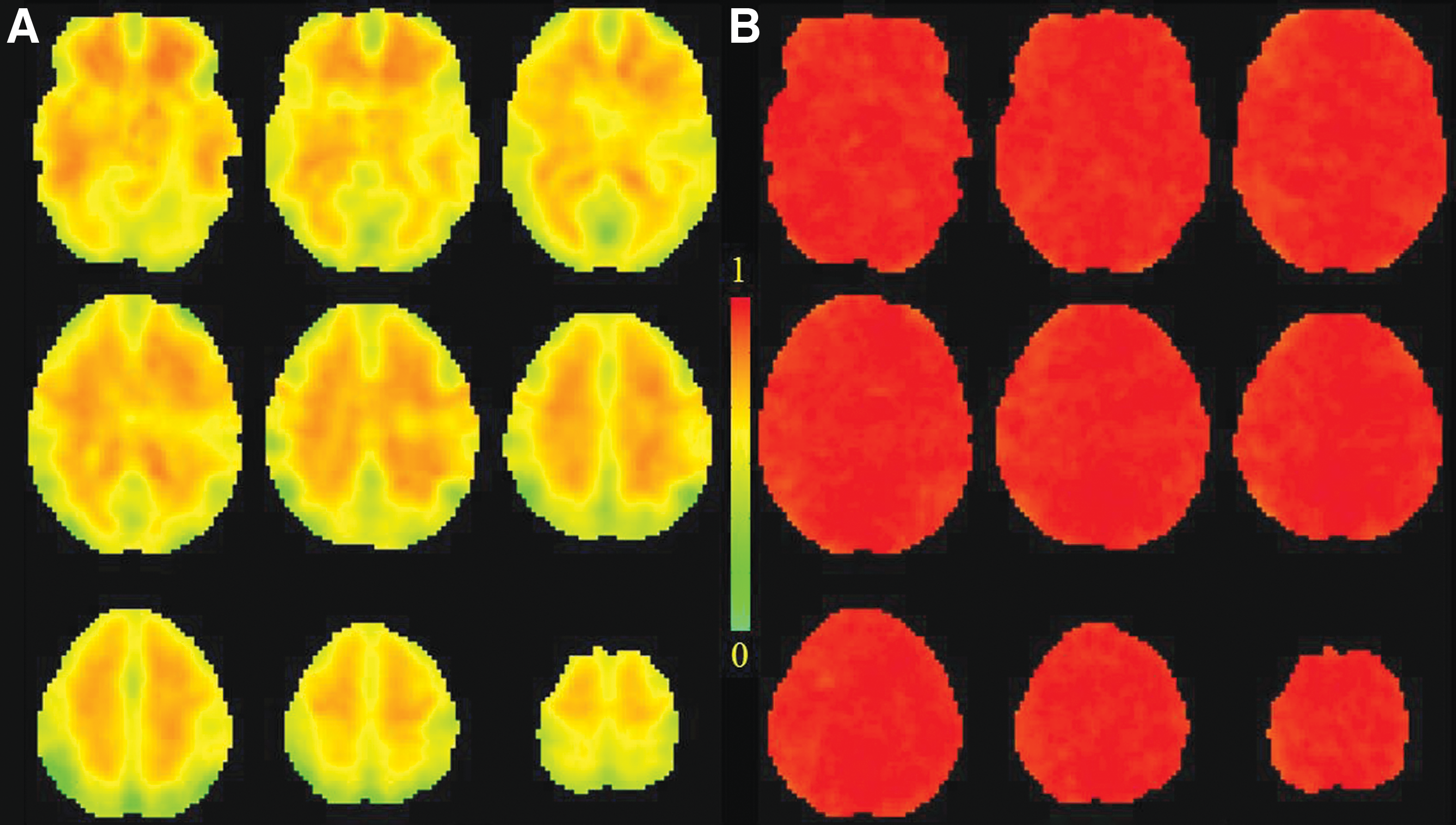
Maps of group-average spatial smoothness (FWHM_ap) in mm across the brain estimated around local neighborhoods (25-mm-radius spheres) for (A) the RSDL_GLS data set and (B) the PC-orthogonalized RSDL-ort80PC data set. Left hemisphere is on the right side of the images. PC, principal component.

FIG. 3.

Maps of the group-average sACF a parameter (which quantifies the Gaussian component of sACF) across the brain estimated around local neighborhoods (25-mm-radius spheres) for (A) the RSDL_GLS data set and (B) PC-orthogonalized RSDL-ort80PC data set. Left hemisphere is on the right side of the images. sACF, spatial autocorrelation function.

Effects of PC orthogonalization on cluster-based FWE correction at different CDTs

Table 2 lists the minimal cluster size thresholds (obtained with 3dClustSim) needed to judge brain activation at different CDTs significant at specific cluster-based FWE-corrected Type 1 error levels (αs), for a putative subject, using sACF parameters obtained from all the RSDL_GLS and RSDL-ort80PC data sets. The “brain mask” used for MC simulations was constructed by multiplying the binary brain masks of all the 21 subjects.

Table 2.

Minimum Cluster Sizes Obtained with 3dClustSim Using MC Simulations Using Noise Characterized by Spatial Correlation Quantified by the Average Mixed Model sACF Parameters Across the Subjects to Judge Brain Activation at Different CDTs Significant at Different FWE Rates (αs) for RSDL_GLS (Top) and RSDL-ort80PC (Bottom) Data Sets

	RSDL_GLS
CDT p-value	α < 0.05	α < 0.03	α < 0.01	α < 0.001
0.05	208 (130)	234 (140)	292 (163)	432 (226)
0.03	122 (85)	137 (92)	170 (105)	248 (180)
0.01	51 (43)	57 (46)	72 (54)	102 (69)
0.001	15 (16)	17 (17)	21 (20)	31 (27)
0.0001	6 (7)	7 (8)	9 (10)	13 (14)

	RSDL-ort80PC
CDT p-value	α < 0.05	α < 0.03	α < 0.01	α < 0.001
0.05	96 (95)	104 (105)	120 (119)	162 (159)
0.03	63 (64)	68 (70)	80 (81)	99 (104)
0.01	33 (33)	35 (35)	41 (40)	51 (50)
0.001	12 (12)	13 (13)	16 (16)	20 (20)
0.0001	6 (6)	6 (6)	8 (8)	11 (10)

The values in the parenthesis denote the cluster size thresholds for the same cell when Gaussian sACF noise with spatial correlation parameterized by FWHM_ap was used during MC simulation.

CDT, cluster detection threshold; FWE, family-wise error; MC, Monte Carlo.

The top half of Table 2 lists the threshold cluster sizes obtained when the spatial correlation of random noise fields for MC simulation was parameterized by the average sACF parameters of RSDL_GLS data sets across 21 subjects. The values in parentheses show the threshold cluster sizes obtained assuming the sACF to be Gaussian (by setting a = 1; and b = FWHM_ap/2.35482). The bottom half of Table 2 lists the corresponding threshold cluster sizes obtained with MC simulation using average sACF parameters of the RSDL-ort80PC data sets.

Table 3 lists the mean and standard deviation of the cluster size thresholds obtained from performing MC simulation on each of the 21 subjects' RSDL_GLS (left) and RSDL-ort80PC (right) data sets, separately with the respective ACF parameters and brain masks obtained from corresponding subjects. Cluster size thresholds obtained from RSDL_GLS data sets, for a given CDT and FWE rate, varied by as much as 15% (standard deviation), whereas the cluster size thresholds obtained from RSDL-ort80PC data sets were almost uniform (maximum standard deviation of cluster size thresholds observed ∼4%) across the different subjects.

Table 3.

Mean (Across 21 Subjects) of the Cluster Size Thresholds Obtained with 3dClustSim Using MC Simulations on Each of the 21 Subjects, Using Noise Characterized by Spatial Correlation Quantified by the Corresponding Subject's Mixed Model sACF Parameters for d CDT p-Values of 0.05, 0.01, and 0.001; and FWE Rate α-Values of 0.05 and 0.01, for RSDL_GLS (Left) and RSDL-ort80PC (Right) Data Sets

	RSDL_GLS		RSDL-ort80PC
CDT p-value	α < 0.05	α < 0.01	α < 0.05	α < 0.01
0.05	222 (30)	313 (50)	99 (4)	120 (5)
0.01	54 (5)	75 (8)	33 (1)	41 (2)
0.001	16 (1)	22 (2)	12 (0)	16 (1)

The values in the parenthesis denote standard deviation across the group for corresponding cluster size thresholds.

Effects of PC orthogonalization on brain activation maps

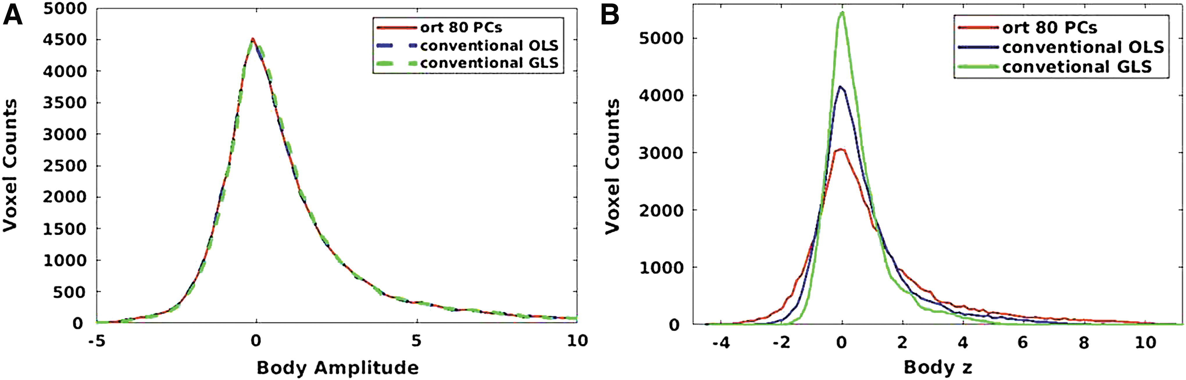
Figure 4 shows the distribution of the average (across 21 subjects). Body category amplitude (Fig. 4A) as well as average group Body z-statistic (Fig. 4B) expressing the strength of brain activation to body-part stimuli. There were no (or imperceptible) differences between the distributions of body amplitude obtained through conventional (both using OLS and GLS approaches) and PC-orthogonalized GLMs, whereas Body z-statistic computed via PC-orthogonalized GLM exhibits longer tails due to the reduction in variance from non-Gaussian signal sources in RSDL-ort80PC data sets.

FIG. 4.

Distribution of average (across 21 subjects) voxel GLM-estimate amplitudes for body condition (A) and average Body z-statistics (B) obtained with the conventional first-level GLM analysis with OLS approach (blue curve), GLS approach (green curve), and PC-orthogonalized GLM (red curve). GLM, general linear model; GLS, generalized least squares; OLS, ordinary least squares.

Figure 5 maps the ratio of the group average Body z-statistic obtained with the optimal PC-orthogonalized GLM to the corresponding average Body z-statistic obtained from conventional GLM using GLS regression, across the brain. This provides an illustration of variations in the increase in detection power engendered by the PC orthogonalization procedure across the brain.

FIG. 5.

Maps of the ratio of Body z-statistic obtained with the optimal PC-orthogonalized GLM to that of the Body z-statistic obtained with the conventional GLM using the GLS approach.

Figure 6 shows the average (across 21 subjects; for representational purposes) Body-Object contrast z-statistic obtained through conventional GLM analysis with OLS approach (Fig. 6A) and GLS approach (Fig. 6C), and with optimal PC orthogonalization using top 80 PCs of the RSDL data sets. The data have been clustered at CDT p < 0.05 and minimum cluster size = 96 voxels (based on 3dClustSim results shown in Table 2), rendering the maps in Figure 6B (but not in Fig. 6A, C) significant at FWE α ≤ 0.05. The PC orthogonalization technique results in detection of two additional clusters of body category-specific activation in the left extrastriate body area (EBA) and superior parietal cortex, respectively.

FIG. 6.

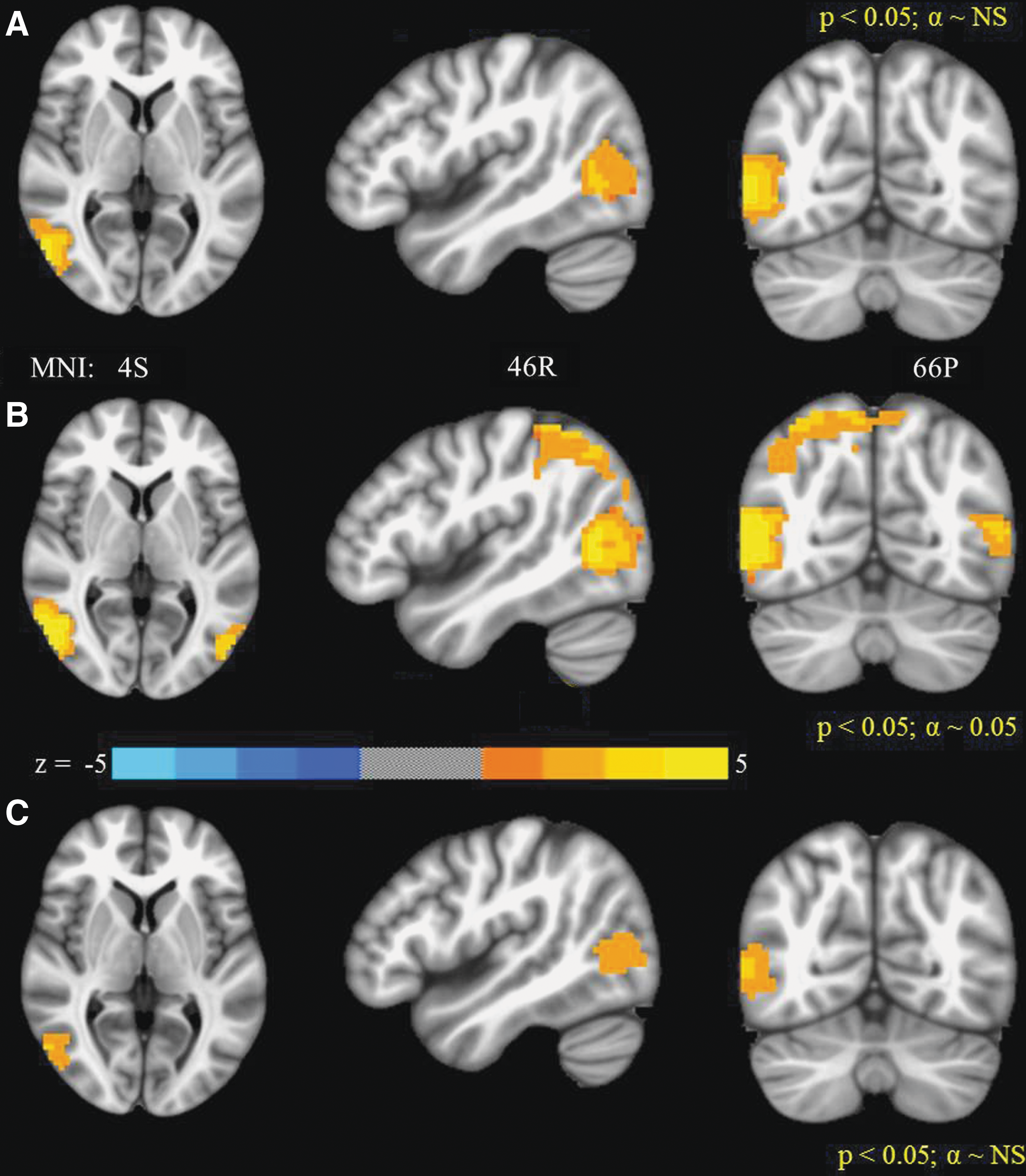
Average (across 21 subjects) of first-level GLM Body-Object t-contrast (converted to standard normal z-statistic) CDT p < 0.05 and cluster size ≥96 voxels using conventional GLM with OLS approach (A), optimal PC-orthogonalized GLM analysis (B), and conventional GLM with GLS approach (C). CDT, cluster detection threshold.

Discussion

As shown in Table 1, the sACF a parameter that quantifies the Gaussian part of the mixed noise sACF model reached its maximum value of 0.994 for all subjects when top 80 or higher 1D PC eigen-time-series were simultaneously orthogonalized during the GLM analysis for this block visual processing fMRI task. Regressing out higher order PCs (i.e., N _opt > 80) reduced the spatial correlation of the corresponding PC-orthogonalized residuals data sets but did not affect sACF a parameter. Furthermore, Table 1 also shows that the spatial correlation range (FWHM_ap) of the data sets did not change appreciably when the numbers of PC eigen-time-series orthogonalized were increased from 70 to 133. This shows that it is not necessary to determine the exact number of PCs required for achieving a Gaussian sACF for each subject.

However, ideally, N _opt should be minimized both to maximize the degrees of freedom in GLM and to ensure that the detrended PCs are not contaminated by white noise. Table 1 also shows that spatial correlation of the RSDL_GLS data sets obtained with conventional GLM using GLS regression was slightly lower than those of the RSDL data sets obtained with conventional GLM using the OLS approach. This indicates that the stochastic ARMA model fitting procedure of the voxel time-series induces a degree of decorrelation to the sACF of the residuals in the GLS approach.

PC orthogonalization renders sACF uniform and Gaussian

The RSDL_GLS data sets (obtained through conventional GLM analysis with GLS approach) exhibited significant heterogeneity in spatial correlation with gray matter areas exhibiting increased spatial smoothness and non-Gaussianity of sACF than white matter areas (Figs. 2A and 3A). The RSDL data sets (obtained through conventional GLM analysis with OLS approach) exhibited even more heterogeneity in spatial correlation than the RSDL_GLS data sets. Consistent with our hypothesis, regressing out signal proportional to non-Gaussian sources that were present in the RSDL data sets through PC orthogonalization under the OLS regression GLM framework yielded first-level analysis GLM residuals (RSDL-ort80PC) with nearly uniform and Gaussian sACF across the brain (Figs. 2B and 3B).

Optimal PC-orthogonalized GLM results in IID OLS regression residuals

The RSDL_GLS data sets generated with conventional GLM analysis exhibited significant departures from normality as assessed with the AD statistics in a significant number of voxels, indicating failure of the ARMA(1,1) stochastic colored noise model to adequately account for temporal correlations in a large number of voxels for some subjects (Fig. 1A). Thus, these residuals voxel time-series did not satisfy the IID criterion required for valid statistical inferences from first-level GLM analysis. Supplementary Figure S1 (Supplementary Data are available online at www.liebertpub.com/brain) shows the RSDL_GLS voxel time-series significantly (voxel p < 0.05) departing from normality for two representative subjects.

In general, the standard stochastic colored noise model failed to adequately account for temporal correlations in brain areas showing large variance in the conventional GLM first-level analysis residuals. However, there was a lot of variability in the fraction of brain voxels exhibiting nonwhite residuals among the RSDL_GLS data sets for different subjects, with percentage of nonwhite voxels in the brain values ranging from 0.25% to 22% across the group. This indicates that the ability of the ARMA model to adequately represent temporal autocorrelation is variable across subjects. However, the GLS approach was superior to the conventional GLM with OLS regression. RSDL data sets (Fig. 1C) consistently yielded a larger number of voxels exhibiting departures of normality in residuals time-series than the RSDL_GLS data sets.

On the contrary, consistent with our expectations, none of the RSDL-ort80PC data sets exhibited voxel time-series that significantly departed from normality as assessed through their AD statistic maps (Fig. 1B). Thus, the PC orthogonalization procedure has the added advantage of rendering the resultant residuals time-series IID, thus satisfying the condition for valid first-level analysis GLM inference. Furthermore, this method of accounting for temporal autocorrelation is superior to the standard method of fitting stochastic colored noise models.

These results also indicate that the sources of temporal autocorrelation in fMRI time-series are indeed nonstochastic signal components such as brain function networks and physiological responses. Thus, this study also introduces a method to obtain whitened GLM first-level analysis residuals, without having to fit ad hoc stochastic colored noise models that incorrectly introduce variance into the residuals, by fitting stochastic models to nonstochastic signal components.

PC orthogonalization reduces minimum cluster sizes needed for FWE correction at different CDTs

As seen in Table 2, the average threshold cluster sizes for FWE correction at different CDTs are much higher for RSDL_GLS data sets, which exhibit large and spatially heterogeneous sACF, than for the RSDL-ort80PC data sets, which exhibit nearly uniform and Gaussian sACF. In fact, recent studies (Cox et al., 2017; Eklund et al., 2016) confirmed by our results in the companion article (Gopinath et al., 2017) suggested that cluster-based FWE correction assuming Gaussian (and even the more conservative mixed model) sACF may not yield valid inferences for the RSDL_GLS data sets (which is obtained with conventional GLM analysis) at CDT p > 0.001.

On the other hand, the sACFs of the RSDL-ort80PC data sets are nearly Gaussian and uniform (which results in very similar threshold cluster sizes for different CDT ps and FWE αs between Gaussian and mixed-model sACFs; Table 2). Hence, based on the results in our companion article (Gopinath et al., 2017), cluster-based FWE correction for PC-orthogonalized GLM analysis should be valid even for CDT p ∼ 0.05. Furthermore, the cluster size thresholds obtained from RSDL_GLS data sets, for the same CDT and FWE rate thresholds, varied appreciably across the subjects (Table 3), whereas the cluster size thresholds obtained from RSDL-ort80PC data sets were more uniform. This indicates that the intrinsic spatial smoothness is similar across subjects. Failure to account for nonstochastic signal components results in artificial variability in detection power across subjects.

PC orthogonalization increases the detection power for individual subject brain activation

The PC orthogonalization technique is designed to make the sACF of the first-level analysis GLM residuals homogeneous and Gaussian by modeling contributions from non-Gaussian sources not related to the fMRI paradigm in addition to task-related activation as separate and orthogonal signal components. This has the added advantage of reducing the variance in the voxel-wise residuals time-series, in addition to making the residuals closer to satisfying IID white noise assumptions underlying the GLM than conventional stochastic noise fitting methods. Thus, although the GLM amplitude estimates obtained with the PC orthogonalization procedure remain unchanged or minimally changed compared with conventional GLM with OLS and GLS approaches, respectively, the detection power of the PC orthogonalization method is enhanced, due to the increased statistical significance of the GLM amplitude estimates (as shown in Figs. 4 and 5).

Figure 5 provides an illustration of variation in the amplification of detection power for the body condition engendered by the PC orthogonalization procedure over the conventional GLM analysis using GLS regression. Supplementary Figure S2 shows this detection power amplification of the PC orthogonalization procedure over the conventional GLM analysis using the OLS approach. The most amplification in detection power (ratio of Body z-statistic between PC-orthogonalized GLM and conventional GLM using GLS or OLS approach) occurred in areas where the variances of RSDL_GLS data set voxels were high. These often coincided with draining veins (especially large sinuses). Furthermore, gray matter voxels, in general, exhibited lot more amplification in detection power than white matter areas.

In the illustrative example of effects of PC orthogonalization presented in Figure 6, PC-orthogonalized GLM analysis (Fig. 6B) results in the Body-Object t-contrast (converted to z-score) map (which expresses the body category-specific activation), exhibiting additional clusters of activation in well-known body-specific areas in the superior parietal cortex (Huang et al., 2012) than just the EBA revealed by conventional GLM analysis using OLS (Fig. 6A) and GLS (Fig. 6C) regression approaches for the same voxel z-statistic and cluster size thresholds.

In fact, when cluster-based FWE correction is applied (through 3dClustSim), only the map shown in Figure 6B is significant at FWE α < 0.05. The conventional GLM analysis with OLS regression results reveals a much smaller cluster of activation (that too only in left EBA; see Supplementary Fig. S3) both due to reduced voxel z-scores and more stringent CDT threshold required to deem the activation significant. The GLS regression-based GLM analysis reveals no activation at all at FWE α < 0.05. The example in Figure 6 is presented for representational purposes. In practice, of course, one should perform FWE-based cluster analysis for each subject separately.

Methodological considerations

The PC orthogonalization method introduced here has been only tested on a block fMRI paradigm in this study. However, this method could also be implemented for event-related fMRI paradigms based on the results mentioned in our companion article (Gopinath et al., 2017), in which detrending signal from non-Gaussian and nonstochastic signal components renders the residuals of GLM analysis in event-related fMRI paradigms exhibit uniform and Gaussian spatial correlation across the brain.

This study was focused on developing a method to obtain first-level analysis GLM residuals with Gaussian sACF and nearly uniform spatial smoothness across the brain for conventional parametric fMRI paradigms. As a result, signals unrelated to the administered fMRI task paradigm (e.g., those arising from coherent fluctuations across specific brain function networks), which introduce spatial correlation, have been treated as nuisance signals and removed through the PC-orthogonalized GLM analysis.

The PCA technique is ideally suited for this method. While independent components analysis (ICA) decomposition is preferable for characterizing non-Gaussian signal components, PCA is optimal where independence of the decomposed signal components is not as important as accounting for the most variance in the RSDL data sets with as small a set of orthogonal signal components as possible. PCs are ordered according to the fraction of net variance in the RSDL data set that is accounted for by each component, with each PC accounting for as much of the data variance as possible. This allows users to develop a figure of merit to determine the minimum number of PCs that will be required to render the sACF nearly Gaussian and spatial smoothness homogenous across the brain, in a convenient and parsimonious manner.

A separate analysis using ICA (with different dimensions) instead of PCA was also used, with similar results (not shown). However, the number of independent components (ICs) needed to account for all non-Gaussian signals was around 100 for all subjects, in contrast to just 80 PCs needed in the PC orthogonalization method proposed. Spatial maps of four ICs obtained from group ICA decomposition of the 21 subject's RSDL data sets are provided in Supplementary Fig. S4 as informative examples. These maps depict three ICs corresponding to well-known brain function networks and one IC, which depicts signal artifacts arising from cerebrospinal fluid fluctuations in the ventricles and large sinuses, adding support to the hypothesis that variance in the RSDL data sets that introduce spatial correlation in the data arises from quantifiable nonstochastic signals.

In general, independent non-Gaussian signal components will be mixed within the PCs due to the nature of the PCA technique. However, as can be seen in Supplementary Figure S5, one can perceive some of the larger brain function networks (e.g., default mode network) intact in some PCs.

While the PC orthogonalization technique renders the spatial structure of first-level GLM residuals nearly uniform and Gaussian, which allows for valid few-corrected inferences to be obtained for less stringent CDTs (e.g., p < 0.05), it must be noted that such clusters can have relatively large spatial extents for FWE α > 0.03 (Table 2), which may detract from making conclusions about brain activation with the specificity desired in some fMRI applications (Woo et al., 2014).

The results also show that the PC orthogonalization technique yields residuals time-series that are IID in time, confirming our hypothesis that autocorrelation in fMRI residuals time-series is caused by nonstochastic signal sources such as brain function networks and physiological responses. However, although the PC orthogonalization technique rendered the residuals time-series of RSDL-ort80PC data sets white and IID in time, it is possible that in some situations, this technique may yield nonwhite residuals in some voxels. This is because the algorithm only examines the whole-brain sACF to determine the number of PCs to orthogonalize from the RSDL data sets. It does not incorporate the temporal correlation in its figures of merit.

Thus, it is possible that certain nonstochastic signals, for example, aliased cardiac fluctuations (Dagli et al., 1999; Glover et al., 2000), may be localized enough in some RSDL-ortN_optPC data sets to not affect the whole-brain sACF calculation and not be apparent in the top N _opt PCs, but still introduce nonstochastic noise into certain voxel residuals time-series. Thus, it is advisable to inspect the normality of the residuals time-series even after PC orthogonalization and use appropriate nonstochastic (e.g., physiological) noise reduction techniques as needed to whiten these voxel time-series.

Finally, since the PC orthogonalization technique does not alter individual GLM-based fMRI activation amplitude estimates, the results of the second-level (group) analysis should not be different from that obtained with conventional parametric fMRI analysis methods. Techniques to account for spatial correlation in second-level analysis residuals arising from non-Gaussian signal sources will be explored in future studies.

Relatedly, since the PC orthogonalization technique only affects the residuals of the first-level GLM analysis, the effects of spatial and temporal correlation introduced by nonstochastic signal components such as brain function networks and physiological responses, on the estimation of the regression parameters, like the amplitude of activation induced by different stimuli, are not alleviated by this technique. However, this drawback is also shared by conventional GLM analysis methods using OLS, and even GLS regression (since stochastic colored noise models are not likely to appropriately account for nonstochastic signal components).

Ideally, one would be able to orthogonalize all nonstochastic sources of signal unrelated to the fMRI paradigm under study during the first pass GLM analysis with OLS approach, as opposed to just orthogonalizing them from first-level residuals (RSDL). However, since ICA (and more so, PCA) component time-series from brain function networks are bound to have considerable correlation with stimulus-related signal in an fMRI task, it may be impossible to achieve this under the aegis of a GLM. It is possible that accurate representation of different neuronal and physiological signal changes induced during an fMRI paradigm will need more sophisticated analysis methods (Lv et al., 2015) than can be afforded by simple parametric fMRI GLMs.

Conclusion

In this study, a simple method to obtain first-level GLM residuals with spatially uniform smoothness and nearly Gaussian sACF was introduced. The results indicate that most of the spatial correlation in fMRI data comes from unmodeled signal from non-Gaussian sources, which can be approximated with PCA-based decomposition and orthogonalized from the task-related signal of interest in conventional parametric fMRI paradigms. As a result, inferences based on conventional cluster-based FWE correction methods, which assume Gaussian sACF, can be rendered valid.

Furthermore, the PC orthogonalization technique was found to be superior to standard stochastic colored noise modeling techniques, in yielding IID in time residuals time-series. Thus, the results also indicate that most of the temporal autocorrelation seen in fMRI time-series arises from unmodeled nonstochastic signal sources. The proposed method also substantially increases the detection power for individual subject-level activation maps.

Footnotes

Acknowledgments

This study was supported by the Department of Radiology and Imaging Sciences, Emory University. Support to K.S. from the Atlanta VAMC is also gratefully acknowledged.

Author Disclosure Statement

No competing financial interests exist.

References

Behzadi

, Liu

. 2006. Caffeine reduces the initial dip in the visual BOLD response at 3 T. Neuroimage, 32:9–15.

Birn

, Diamond

, Smith

, Bandettini

. 2006. Separating respiratory-variation-related fluctuations from neuronal-activity-related fluctuations in fMRI. Neuroimage, 31:1536–1548.

Bracci

, Ietswaart

, Peelen

, Cavina-Pratesi

. 2010. Dissociable neural responses to hands and non-hand body parts in human left extrastriate visual cortex. J Neurophysiol, 103:3389–3397.

Buckner

, Sepulcre

, Talukdar

, Krienen

, Liu

, Hedden

, et al. 2009. Cortical hubs revealed by intrinsic functional connectivity: mapping, assessment of stability, and relation to Alzheimer's disease. J Neurosci, 29:1860–1873.

Bullmore

, Brammer

, Williams

, Rabe-Hesketh

, Janot

, David

, et al. 1996. Statistical methods of estimation and inference for functional MR image analysis. Magn Reson Med, 35:261–277.

Buxton

. 2009. Introduction to Functional Magnetic Resonance Imaging: Principles and Techniques, 2nd edition. New York, NY: Cambridge University. Press.

Carmack

, Spence

, Schucany

, Gunst

, Lin

, Haley

. 2012. A new class of semiparametric semivariogram and nugget estimators. Computat Stat Data Anal, 56:1737–1747.

Chang

, Cunningham

, Glover

. 2009. Influence of heart rate on the BOLD signal: the cardiac response function. Neuroimage, 44:857–869.

Cox

. 1996. AFNI: software for analysis and visualization of functional magnetic resonance neuroimages. Comput Biomed Res, 29:162–173.

10.

Cox

, Chen

, Glen

, Reynolds

, Taylor

. 2017. FMRI Clustering in AFNI: False-Positive Rates Redux. Brain Connect, 7:152–171.

11.

Crosson

, McGregor

, Gopinath

, Conway

, Benjamin

, Chang

, et al. 2007. Functional MRI of language in aphasia: a review of the literature and the methodological challenges. Neuropsychol Rev, 17:157–177.

12.

Crosson

, Moore

, Gopinath

, White

, Wierenga

, Gaiefsky

, et al. 2005. Role of the right and left hemispheres in recovery of function during treatment of intention in aphasia. J Cogn Neurosci, 17:392–406.

13.

Dagli

, Ingeholm

, Haxby

. 1999. Localization of cardiac-induced signal change in fMRI. Neuroimage, 9:407–415.

14.

Eklund

, Nichols

, Knutsson

. 2016. Cluster failure: why fMRI inferences for spatial extent have inflated false-positive rates. Proc Natl Acad Sci U S A, 113:7900–7905.

15.

Epstein

, Higgins

. 2007. Differential parahippocampal and retrosplenial involvement in three types of visual scene recognition. Cereb Cortex, 17:1680–1693.

16.

Fair

, Schlaggar

, Cohen

, Miezin

, Dosenbach

, Wenger

, et al. 2007. A method for using blocked and event-related fMRI data to study “resting state” functional connectivity. Neuroimage, 35:396–405.

17.

Fredholm

, Battig

, Holmen

, Nehlig

, Zvartau

. 1999. Actions of caffeine in the brain with special reference to factors that contribute to its widespread use. Pharmacol Rev, 51:83–133.

18.

Friston

, Glaser

, Henson

, Kiebel

, Phillips

, Ashburner

. 2002. Classical and Bayesian inference in neuroimaging: applications. Neuroimage, 16:484–512.

19.

Glover

, Li

, Ress

. 2000. Image-based method for retrospective correction of physiological motion effects in fMRI: RETROICOR. Magn Reson Med, 44:162–167.

20.

Gopinath

, Krishnamurthy

, Sathian

. 2017. Accounting for non-Gaussian sources of spatial correlation in parametric fMRI paradigms I: revisiting cluster-based inferences. Brain Connect [Epub ahead of print] DOI: 10.1089/brain.2017.0521

21.

Gopinath

, Lacey

, Ahmed

, Stilla

, Sathian

. 2013. Resting-state functional connectivity of specialized occipitotemporal cortical regions. Proc ISMRM, 21:2254.

22.

Huang

, Chen

, Tran

, Holstein

, Sereno

. 2012. Mapping multisensory parietal face and body areas in humans. Proc Natl Acad Sci U S A, 109:18114–18119.

23.

Kanwisher

, McDermott

, Chun

. 1997. The fusiform face area: a module in human extrastriate cortex specialized for face perception. J Neurosci, 17:4302–4311.

24.

Katz

, Garst

, Briggs

, Cheshkov

, Ringe

, Gopinath

, et al. 2012. Neural bases of the foreign accent syndrome: a functional magnetic resonance imaging case study. Neurocase, 18:199–211.

25.

Liau

, Perthen

, Liu

. 2008. Caffeine reduces the activation extent and contrast-to-noise ratio of the functional cerebral blood flow response but not the BOLD response. Neuroimage, 42:296–305.

26.

Liu

, Behzadi

, Restom

, Uludag

, Lu

, Buracas

, et al. 2004. Caffeine alters the temporal dynamics of the visual BOLD response. Neuroimage, 23:1402–1413.

27.

, Jiang

, Li

, Zhu

, Zhang

, Zhao

, et al. 2015. Holistic atlases of functional networks and interactions reveal reciprocal organizational architecture of cortical function. IEEE Trans Biomed Eng, 62:1120–1131.

28.

Malach

, Reppas

, Benson

, Kwong

, Jiang

, Kennedy

, et al. 1995. Object-related activity revealed by functional magnetic resonance imaging in human occipital cortex. Proc Natl Acad Sci U S A, 92:8135–8139.

29.

Nehlig

. 1999. Are we dependent upon coffee and caffeine? A review on human and animal data. Neurosci Biobehav Rev, 23:563–576.

30.

Nehlig

, Boyet

. 2000. Dose-response study of caffeine effects on cerebral functional activity with a specific focus on dependence. Brain Res, 858:71–77.

31.

Power

, Barnes

, Snyder

, Schlaggar

, Petersen

. 2012. Spurious but systematic correlations in functional connectivity MRI networks arise from subject motion. Neuroimage, 59:2142–2154.

32.

Purdon

, Solo

, Weisskoff

, Brown

. 2001. Locally regularized spatiotemporal modeling and model comparison for functional MRI. Neuroimage, 14:912–923.

33.

Sahib

, Mathiak

, Erb

, Elshahabi

, Klamer

, Scheffler

, et al. 2016. Effect of temporal resolution and serial autocorrelations in event-related functional MRI. Magn Reson Med, 76:1805–1813.

34.

Smith

, Jenkinson

, Woolrich

, Beckmann

, Behrens

, Johansen-Berg

, et al. 2004. Advances in functional and structural MR image analysis and implementation as FSL. Neuroimage 23 Suppl, 1:S208–S219.

35.

Stephens

. 1974. EDF statistics for goodness of fit and some comparisons. J Am Stat Assoc, 69:730–737.

36.

Thesen

, Heid

, Mueller

, Schad

. 2000. Prospective acquisition correction for head motion with image-based tracking for real-time fMRI. Magn Reson Med, 44:457–465.

37.

Turk-Browne

. 2013. Functional interactions as big data in the human brain. Science, 342:580–584.

38.

Woo

, Krishnan

, Wager

. 2014. Cluster-extent based thresholding in fMRI analyses: pitfalls and recommendations. Neuroimage, 91:412–419.

Supplementary Material

Please find the following supplemental material available below.

For Open Access articles published under a Creative Commons License, all supplemental material carries the same license as the article it is associated with.

For non-Open Access articles published, all supplemental material carries a non-exclusive license, and permission requests for re-use of supplemental material or any part of supplemental material shall be sent directly to the copyright owner as specified in the copyright notice associated with the article.

0.00 MB

0.70 MB