Anti-Fragmentation of Resting-State Functional Magnetic Resonance Imaging Connectivity Networks with Node-Wise Thresholding

Abstract

Functional magnetic resonance imaging (fMRI)-based functional connectivity networks are often constructed by thresholding a correlation matrix of nodal time courses. In a typical thresholding approach known as hard thresholding, a single threshold is applied to the entire correlation matrix to identify edges representing superthreshold correlations. However, hard thresholding is known to produce a network with uneven allocation of edges, resulting in a fragmented network with a large number of disconnected nodes. It is suggested that an alternative network thresholding approach, node-wise thresholding, is able to overcome these problems. To examine this, various network characteristics were compared between networks constructed by hard thresholding and node-wise thresholding, with publicly available resting-state fMRI data from 123 healthy young subjects. It was found that networks constructed with hard thresholding included a large number of disconnected nodes, while such network fragmentation was not observed in networks formed with node-wise thresholding. Moreover, in hard thresholding networks, fragmentized modular organization was observed, characterized by a large number of small modules. On the contrary, such modular fragmentation was not observed in node-wise thresholding networks, producing modules that were robust at any threshold and highly consistent across subjects. These results indicate that node-wise thresholding may lead to less fragmented networks. Moreover, node-wise thresholding enables robust characterization of network properties without much influence by the selection of a threshold.

Introduction

A functional connectivity network can be constructed by correlating nodal time courses from functional magnetic resonance imaging (fMRI) time series data. In particular, a cross-correlation matrix describing linear correlations between all node pairs is calculated, and edges are defined based on the magnitude of correlation coefficients. Although it is possible to construct a weighted network by ascribing the correlation value to each edge, the vast majority of fMRI connectivity networks are constructed by thresholding the correlation matrix to identify strong correlations between nodes. Any correlation above the threshold is interpreted as functional connectivity, represented by an edge in the resulting network.

In a widely used network construction method, a single threshold is applied to the entire correlation matrix to identify edges. The use of a single threshold, also known as hard thresholding, is motivated to identify strong correlations among a large number of correlation coefficients. Identifying a small number of true effects among a large number of statistic values is a common problem in a statistical analysis of neuroimaging data, in which a statistical test is performed at each voxel separately. The use of hard thresholding may be viewed as an extension of this problem in a correlation analysis (Worsley et al., 1998). There are several ways to select a threshold for hard thresholding. The threshold may be adjusted to control the proportion of edges above the threshold (or sparsity) (Wang et al., 2009), the average number of connections (or degree) (van den Heuvel et al., 2008; Wang et al., 2009), or the false discovery rate (Bassett et al., 2006). In hard thresholding, each correlation coefficient is treated the same, and dichotomized into either a strong correlation (thus an edge) or a weak correlation (thus absence of an edge) based on the predefined criterion as described above.

Although each edge is formed based on a statistical principle in hard thresholding, the resulting edges collectively do not describe a network appropriately. In particular, edges are unevenly distributed in the resulting network. Edges tend to concentrate among highly connected nodes, while a large portion of nodes may be isolated or sparsely connected (Foti et al., 2011; Ruan et al., 2010). This is an inherent problem in networks formed by hard thresholding a correlation matrix, not just functional connectivity networks. Figure 1 shows an example of this. A stock price correlation network is formed by thresholding a correlation matrix of stock price time series of 491 companies [see Hayasaka (2016) for details]. With hard thresholding, edges are concentrated among a subset of highly connected companies, while a large number of companies are disconnected from the network (Fig. 1a). Even when 90% of nodes are connected to the main network, edges are still concentrated to a subset of network nodes (Fig. 1b).

FIG. 1.

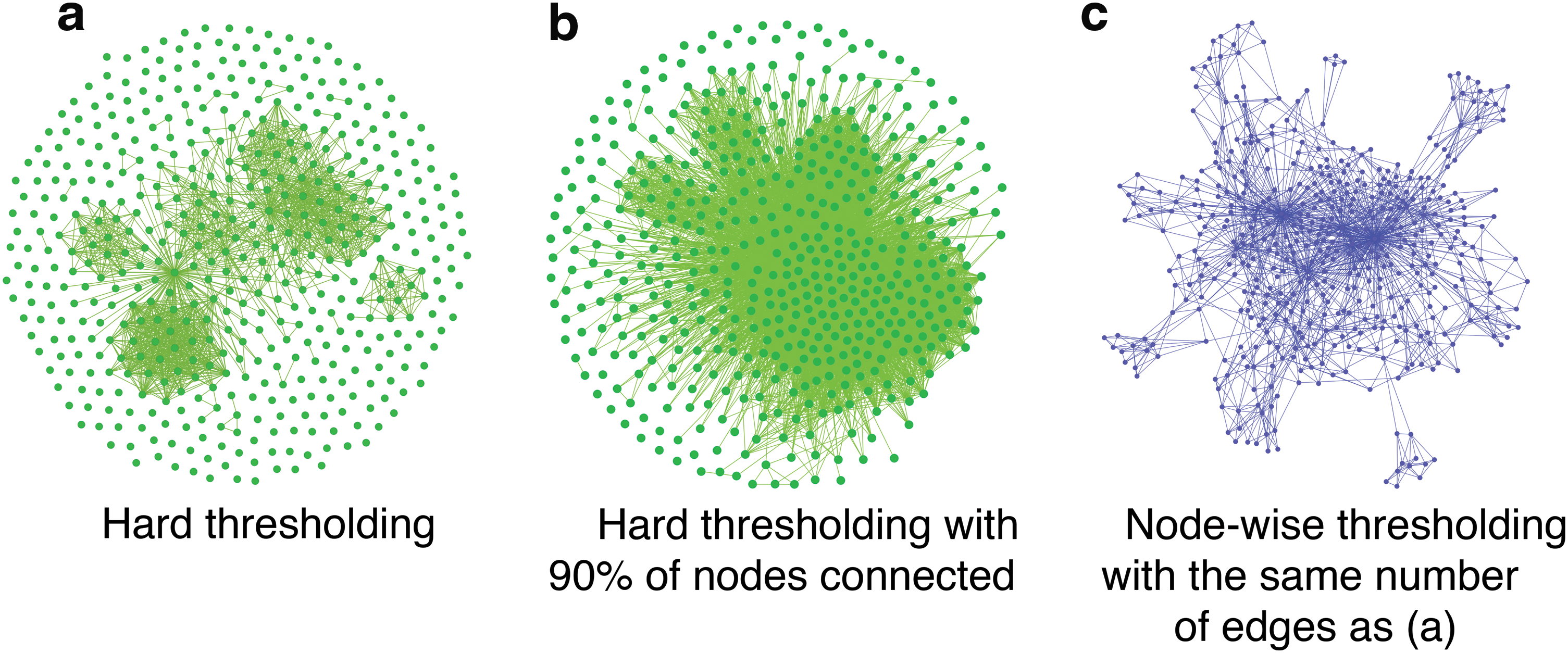
Examples of network thresholding methods applied to the stock market correlation data with n = 491 nodes (Hayasaka, 2016). In a network formed by hard thresholding (a), edges concentrate only on a small portion of nodes, while the majority of the nodes are disconnected. Even with 90% nodes connected to the giant component (b), hard thresholding still leaves a number of disconnected or sparsely connected nodes. On the contrary, a network formed by node-wise thresholding has virtually no disconnected nodes (c), even with as few edges as the example shown (a). Color images available online at www.liebertpub.com/brain

Some may argue that these networks demonstrate characteristics of typical self-organized networks, with a small number of high-degree hub nodes, while the vast majority of nodes have low degrees (Barabasi and Albert, 1999). High-degree hubs are relatively rare in real networks, but in a network formed by hard thresholding (as seen in Fig. 1), high-degree hubs are far more abundant, more so when there are a large number of edges (Fig. 1b). Hard thresholding also results in a fragmented network with a large proportion of disconnected nodes. Many nodes are disconnected despite a large number of edges (Fig. 1b).

To overcome the problems of hard thresholding as described above, one can apply a threshold at each node separately. In particular, one can threshold each row of a correlation matrix separately, controlling the number of edges (Ruan et al., 2010) or the proportion of the superthreshold edges (Foti et al., 2011) at each node. This thresholding approach, referred as node-wise thresholding, still follows a statistical principle of selecting strong correlation as edges, as done in hard thresholding. The only difference is that edges are identified at each node separately in node-wise thresholding. In a network formed by node-wise thresholding, edges are more evenly distributed throughout the network without any concentration among a subset of nodes. For example, the network shown in Figure 1c, formed by node-wise thresholding, has the same number of edges as the network shown in Figure 1a. It can be seen from the figure that almost all the nodes are connected as a single network. In fact, networks formed by node-wise threshold undergo a phase-transition phenomenon known as percolation during network formation as edges are introduced. In percolation, the largest connected component (known as the giant component) grows dramatically from a fragmented state to the point where almost all nodes are connected. High-degree hub nodes still exist in a node-wise thresholding network, but far fewer than a hard thresholding network of the same number of nodes and edges. Thus, node-wise thresholding may solve the problems associated with hard thresholding, namely uneven allocation of edges and network fragmentation.

To demonstrate the utility of node-wise thresholding in constructing fMRI connectivity networks, I examine the characteristics of networks formed by node-wise thresholding and compare to that of networks formed by hard thresholding. A particular focus is given to anti-fragmentation property of node-wise thresholding. How does the giant component grow? Are edges evenly allocated throughout the network? In addition, I examine whether the networks formed by node-wise thresholding are modular, comprising clusters of highly interconnected nodes known as modules. I compare network modular organization between node-wise thresholding and hard thresholding networks. I used resting-state fMRI data from n = 123 individuals from the 1000 Functional Connectomes Project. Networks were generated at the regions of interest (ROI) level with parcellation defined by the automated anatomical labeling (AAL) atlas (Tzourio-Mazoyer et al., 2002), as well as at the voxel level. The modular organization analysis results focus mainly on voxel-based networks.

Materials and Methods

Data

Publicly available resting-state fMRI data were used in this project. In particular, six data sets from six sites were obtained from the 1000 Functional Connectomes Project (1000FCP; http://fcon_1000.projects.nitrc.org). Total of n = 123 subjects were included in the analysis for this project, originating from Berlin (n = 26, M/F = 13/13), Leiden (n = 19, M/F = 11/8), Newark (n = 18, M/F = 9/9), New York (n = 20, M/F = 8/12), Oxford (n = 22, M/F = 12/10), and Queensland (n = 18, M/F = 11/7). These data sets comprised resting-state fMRI data from young (18–46 years old) healthy subjects acquired while eyes open, along with a high-resolution T1-weighted structural MRI image for each subject. The number of time points for the fMRI data varied between sites, ranging from 135 (Newark) to 215 (Leiden). Details on the fMRI data sets can be found from the 1000FCP website.

fMRI data processing

Before the preprocessing of fMRI data, the first 3 volumes were deleted from each subject's fMRI data for steady-state magnetization. The fMRI time series consisting of the remaining time points was then aligned to the middle time point to correct any displacement during the scan. The aligned fMRI data were then coregistered to the subject's T1-weighted structural MRI data by a six-parameter rigid body transformation. The structural image was spatially normalized to the MNI (Montréal Neurological Institute) template with a 12-parameter affine transformation and a nonlinear registration. The resulting spatial warping was then applied to the fMRI data to normalize it to the template space. Each 3D volume in the normalized fMRI time series data was then resliced to a 3D matrix of 46 × 55 × 42 voxels of 4 × 4 × 4 mm cube. These steps were carried out using FSL5.0 (The Oxford Centre for Functional Magnetic Resonance Imaging of the Brain, Oxford, UK) (Jenkinson et al., 2012; Smith et al., 2004).

The normalized fMRI time series data were band-pass filtered (0.009–0.08 Hz) to reduce physiological and scanner noises (Fox et al., 2005; Van Dijk et al., 2010). From the filtered fMRI time series data, some confounding time series were regressed out, including the six realignment parameters from the rigid body transformation, as well as the mean time courses from the brain parenchyma, deep white matter, and cerebrospinal fluid voxels (Hayasaka, 2013; Hayasaka and Laurienti, 2010). The filtered and regressed fMRI data were then scrubbed for excessive motion, using the frame displacement (FD) criterion of FD >0.5 (Power et al., 2012). The resulting fMRI data were then masked to include gray matter areas in the AAL atlas (Tzourio-Mazoyer et al., 2002) as well as the subject's own parenchyma mask. Finally, the mean time course was extracted in 90 ROIs in the cerebrum defined by the AAL atlas.

Based on the preprocessed data, two correlation matrices were calculated for each subject: (1) a voxel-level correlation matrix of ∼19,000 × 19,000 with each gray matter voxel representing a node and (2) an ROI-based correlation matrix of 90 × 90 with each ROI representing a node. The band-pass filtering, regression, motion scrubbing, masking, ROI extraction, and calculation of correlation matrices were implemented by custom scripts in Python. Interested readers can download the Python codes used in this article from a GitHub repository (https://github.com/sathayas/fMRIConnectome). The main diagonal elements of a resulting correlation matrix were set to zero to avoid self-loops during network construction.

Network construction

A node-wise thresholding network was constructed by selecting d largest correlation coefficients on each row of the correlation matrix (Hayasaka, 2016; Ruan et al., 2010). For voxel-based networks, networks were constructed for d = 3, 4, 5, 6, 8, 10, 15, 20, and 30. For ROI-based network, networks were constructed for d = 1, 2, 3, 4, 5, 6, 8, 10, and 15. It should be noted that the degree at each node is not necessarily d. Even if an edge (i,j) is attributed to one of the top d correlations for node i, it may not be part of the top d correlations for node j. This results in the node degree of j greater than d. Thus, in the resulting network, the minimum node degree is d but node degrees can range dramatically. In fact, as it can be seen from degree distributions below, there is a wide variety of node degrees in a node-wise thresholding network. Moreover, local variability in node degrees can be observed, with concentrations of highly connected nodes in certain brain areas.

To facilitate a comparison with node-wise thresholding networks, hard thresholding networks were constructed by adjusting the threshold in a way that the number of edges is the same as the node-wise thresholding network with a particular value of d. Needless to say that node-wise thresholding networks and hard thresholding networks were derived from the same set of correlation matrices; only the thresholding method differed between the two types of networks.

Network characteristics

Various network metrics were calculated and compared between the networks constructed by node-wise thresholding and by hard thresholding. The metrics included the relative giant component size G (the number of nodes connected to the giant component divided by the number of all nodes), the characteristic path length L (the average shortest distance between any pairs of nodes), and the clustering coefficient C (the average probability that two nodes connected to a particular node are also connected to each other). For the calculation of L, only the nodes in the giant component were included. The formulae for C and L can be found in Rubinov and Sporns (2010) and Stam and Reijneveld (2007). The network metrics were compared by paired t-tests between node-wise thresholding networks and hard thresholding networks at different values of d.

In addition to the network metrics, node degrees were also examined. The degree distributions were generated for different types of networks (node-wise thresholding and hard thresholding) at different values of d. In addition, the consistency of the hub nodes was examined. In particular, the spatial overlap maps of hub node locations were generated. Hubs were defined as the nodes with top 20% highest degrees, in the spirit of the 80–20 rule by Pareto (Hayasaka and Laurienti, 2010).

Modular organization

For voxel-based networks, modular organization was examined. In particular, the giant component of each network was parcellated into modules by the Louvain method (Blondel et al., 2008). The resulting modularity Q, the metric describing the quality of modular parcellation [see Newman (2006a, 2006b) and Newman and Girvan (2004) for the formula], was calculated and compared between the thresholding methods (node-wise thresholding vs. hard thresholding). In addition, the number of modules and the median module size were also compared between the thresholding methods with paired t-tests at different values of d. Finally, the consistency of the default mode network (DMN) module and the sensory motor (SM) module was compared between the thresholding methods. In particular, for each network, a DMN module was identified as the module with the largest spatial overlap, measured by the Jaccard index (the ratio of the intersection to the union), with the following ROIs: bilateral medial orbitofrontal cortex, posterior cingulate gyrus, precuneus, and angular gyrus. Similarly, an SM module was identified as the module with the largest spatial overlap with the bilateral pre- and postcentral gyri. Binary images for the DMN module and the SM module were produced for each network for each subject, indicating the module with 1 sec. Then, the binary images were summed across subjects, producing the overlap map of the DMN module and the SM module for different thresholding methods and different values of d. The DMN and SM modules were chosen since they are known to be consistent across subjects (Moussa et al., 2011).

Aside from being highly consistent across subjects, the SM module was chosen to assess the modular parcellation accuracy for two additional reasons. First, the main constituents of the SM module, the sensory and motor cortices, have been extensively examined in vivo in humans by direct electrical stimulation since the early 1900s (Borchers et al., 2011), with well-delineated boundaries. Second, the functional connectivity between the bilateral sensory and motor cortices has been documented since the earliest report of functional connectivity by Biswal and coworkers (1995). A numerous seed-based connectivity and independent component analysis studies have demonstrated the correlated BOLD signals in these areas. For these reasons, I considered the SM module to be a module with the known ground truth. If the sensory and motor cortices are part of a single module in most subjects, then the consistency of the SM module should be elevated in these brain areas. On the contrary, if the SM module does not cover the sensory and motor cortices in their entirety in a large portion of subjects, then the consistency for the SM module will be diminished. This is because each subject's SM module covers only some parts of the sensory and motor cortices, and the coverage may not overlap across subjects.

Results

Network statistics

Figure 2 shows the mean and standard deviation (SD) of network statistics for voxel-based networks and ROI-based networks, formed by the two thresholding methods. There are three notable findings from the network statistics.

FIG. 2.

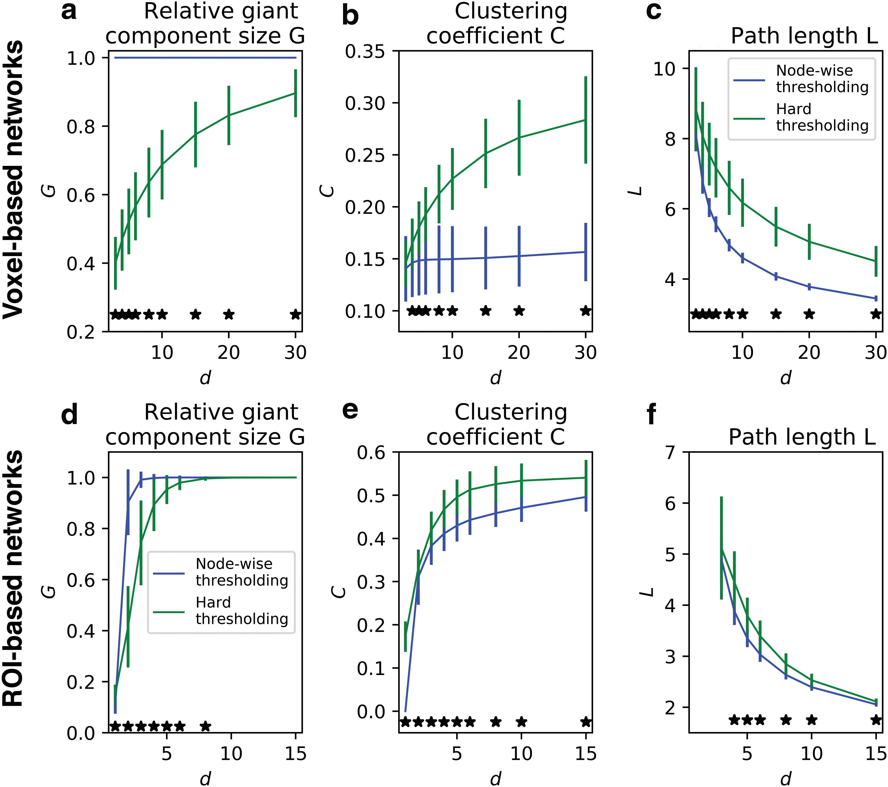
The mean and SD of various characteristics of networks formed by different thresholding methods (node-wise thresholding or hard thresholding) over a range of d. The results for the voxel-based networks are shown on the top row, whereas the results for the ROI-based networks are shown on the bottom row. The relative giant component size G (a, d), the clustering coefficient C (b, e), and the path length L (c, f) are shown. Network characteristics were compared between the two thresholding methods by paired t-tests for each d. Significant differences between the thresholding methods (p < 0.05, Bonferroni corrected across d) are indicated by stars. ROI, regions of interest; SD, standard deviation. Color images available online at www.liebertpub.com/brain

First, the relative giant component size G was almost 1 for d ≥ 3 for node-wise thresholding networks, whereas G did not approach 1 for hard thresholding networks unless d was large. See Figure 2a for voxel-based networks and Figure 2d for ROI-based networks. G was close to 1 for node-wise networks due to a phase-transition phenomenon known as percolation, in which fragmented network components coalesce into a giant component comprising a majority of nodes with an introduction of a small number of edges. It has been reported that, for networks formed by node-wise thresholding, percolation occurs somewhere between d = 2 and 3 (Hayasaka, 2016). Hard thresholding networks, in contrast, do not undergo such a system-wide network formation phenomenon. The giant component grew only incrementally as edges were added as d increased. While G eventually reached 1 for ROI-based hard thresholding networks for sufficiently large d, G did not reach 1 for voxel-based counterparts. Even with d = 30, G was around 90%, indicating that about 10% nodes were still fragmented in hard thresholding networks.

Second, the clustering coefficient C was always higher for hard thresholding networks compared to node-wise thresholding networks, more so for larger d. See Figure 2b for voxel-based networks, and Figure 2e for ROI-based networks. Interestingly, for voxel-based networks, C seemed to plateau for node-wise thresholding networks, whereas C increased as d increased in hard thresholding networks. Higher C is an indication of a larger number of triangles in a network. Thus, an introduction of more edges (associated with an increase in d) likely results in formation of more triangles, possible redundant connections, in hard thresholding networks compared to node-wise thresholding networks.

Third, the path length L was always shorter for node-wise thresholding networks compared to hard thresholding networks. See Figure 2c for voxel-based networks, and Figure 2f for ROI-based networks. This means the average distance between any node pair is shorter for node-wise thresholding networks, indicating more global integration as a network as a whole.

Node degree distribution

Figure 3 shows node degree distributions of the voxel-based and ROI-based networks (Fig. 3a, b, c, and d, respectively) formed by node-wise thresholding (Fig. 3a, c) and hard thresholding (Fig. 3b, d), at various values of d. In particular, the complementary cumulative distribution function [1 − F(k_i )] was plotted against the node degree k_i . Each degree distribution was a combined distribution of n = 123 subjects. For networks formed with node-wise thresholding, the shape of the distribution was similar across the range of d. In other words, the relative abundance (or scarcity) of low-degree (or high-degree) nodes was preserved across different values of d. This was observed in both voxel-based and ROI-based networks (Figure 3a, c, respectively).

FIG. 3.

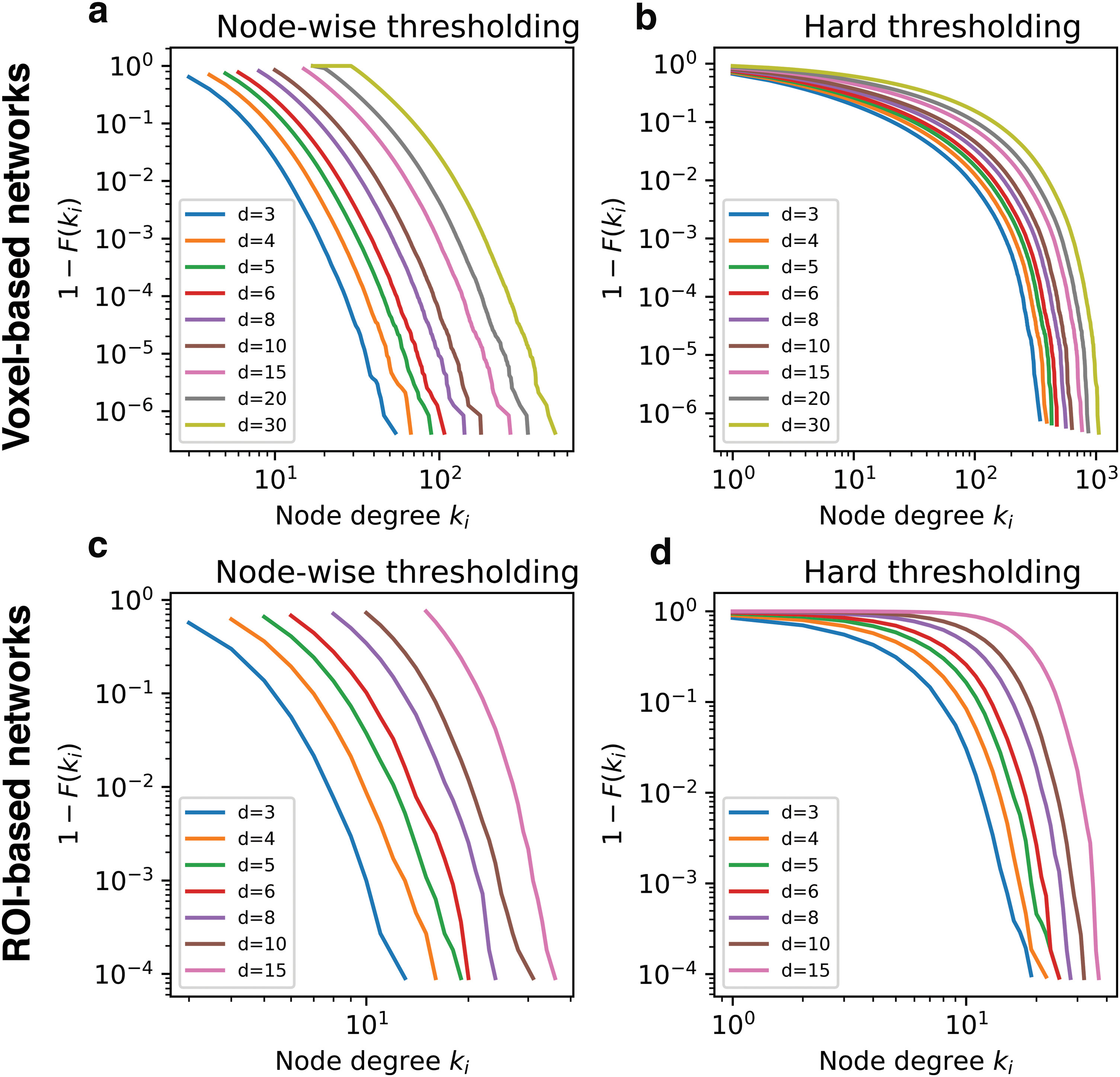
Degree distributions of node-wise thresholding networks (a, c) and hard thresholding networks (b, d) formed at different values of d. Degree distributions from voxel-based networks are shown on the top row, and degree distributions from ROI-based networks are show on the bottom row. Each degree distribution is a combined distribution of n = 123 networks. Color images available online at www.liebertpub.com/brain

On the contrary, the shape of the distribution changed with different values of d for hard thresholding networks. In particular, an increase in d was associated with increased curvature of the degree distribution. This is consistent with a previous report on degree distributions at different sparsity (Fornito et al., 2010). The increased curvature indicated that the relative abundance of medium- to high-degree nodes increases as d increases, whereas low-degree nodes become less abundant. In other words, additional edges associated with an increase in d seem to be allocated among already highly connected nodes, as it can be seen in Figure 1b.

Consistency of high-degree nodes

The consistency of high-degree nodes, or hubs, across n = 123 subjects was examined. In particular, top 20% highest degree nodes were identified in each subject's network, and their spatial overlap was examined across subjects (Fig. 4). For voxel-based networks, high-degree nodes were consistent in the posterior cingulate, precuneus, angular gyrus, and medial prefrontal cortex (Fig. 4a). These areas constitute a collection of brain areas known as the DMN (Raichle and Snyder, 2007), and the results were similar to previous voxel-level resting-state fMRI network studies (Hayasaka and Laurienti, 2010; Power et al., 2011; van den Heuvel et al., 2008). Both thresholding methods produced similar areas of overlap and did not vary much across d. However, the spatial extent and the magnitude of overlap were larger in the hard thresholding networks. This may be due to concentration of edges among high-degree nodes, as seen in Figure 1b. For ROI-based networks, high-degree nodes were consistent in the medial prefrontal cortex, insula, superior temporal gyrus, and operculum (Fig. 4b). For low d, a strong overlap was also found in the posterior cingulate and in the occipital lobe. The results were similar between the thresholding methods.

FIG. 4.

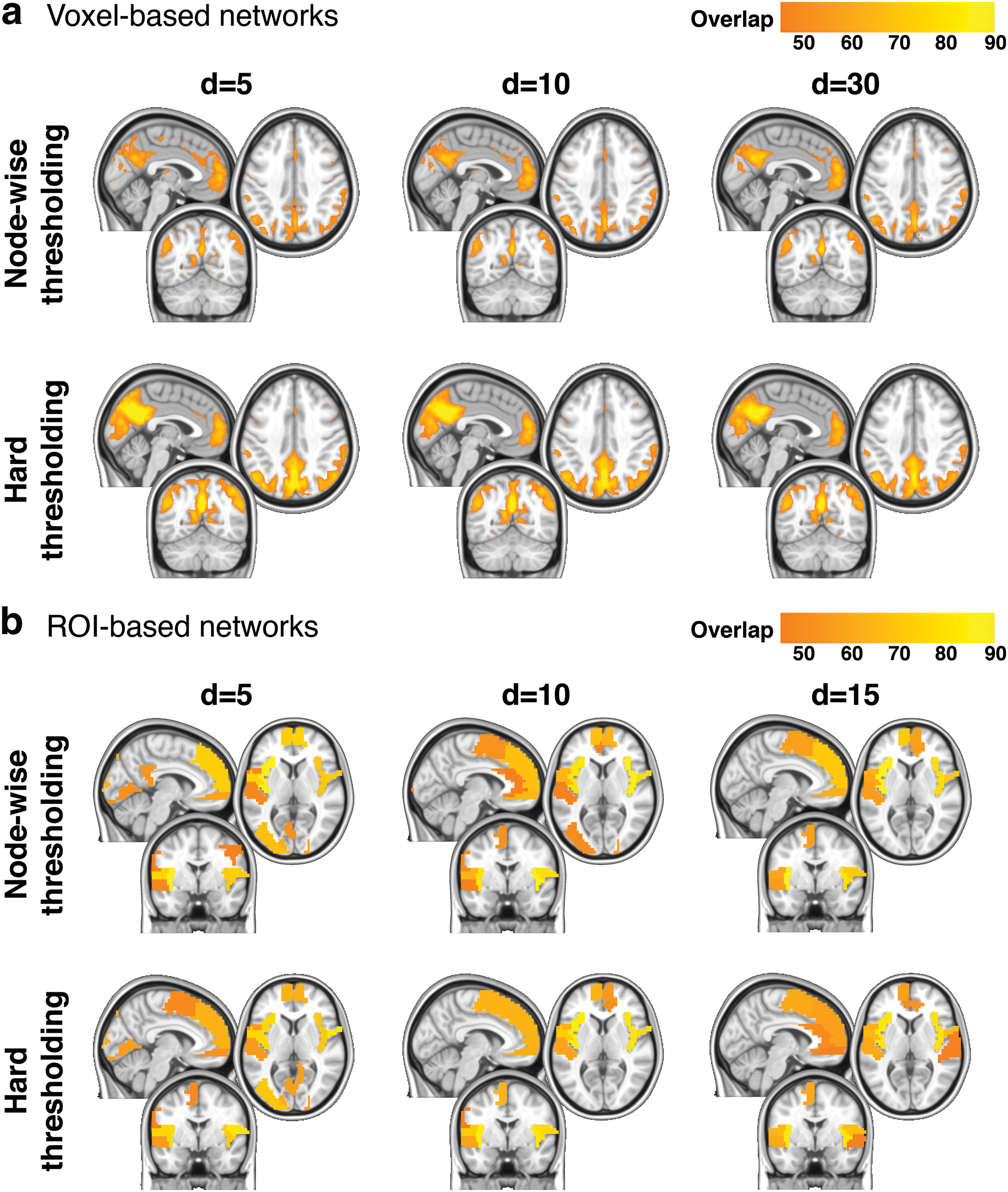
Consistency of high-degree nodes. The locations of top 20% highest degree nodes were identified in each subject's network, and the overlap of the high-degree node locations is visualized for voxel-based networks (a) and ROI-based networks (b). The overlap maps were calculated for different thresholding methods, node-wise thresholding (top) and hard thresholding (bottom) at different values of d. For voxel-based networks, overlap maps are shown for d = 5, 10, and 30. For ROI-based networks, overlap maps are shown for d = 5, 10, and 15. Color images available online at www.liebertpub.com/brain

Modular organization

Figure 5 shows the mean and SD of various statistics associated with modular parcellation of voxel-based networks across different values of d and different thresholding methods. The modularity Q, the statistic indicating the modular tendency of a network, was higher among hard thresholding networks compared with node-wise thresholding networks (Fig. 5a, p < 0.05 Bonferroni corrected). However, hard thresholding networks had a considerably larger number of modules compared with node-wise thresholding networks (Fig. 5b, p < 0.05 Bonferroni corrected). Moreover, the median module size is much smaller among hard thresholding networks compared with node-wise thresholding networks (Fig. 5c, p < 0.05 Bonferroni corrected). These results suggest that hard thresholding networks may have a large number of small modules, and the existence of such small modules may be driving the higher modularity Q, since the calculation of modularity does not penalize a large number of modules (Newman, 2006a, 2006b; Newman and Girvan, 2004).

FIG. 5.

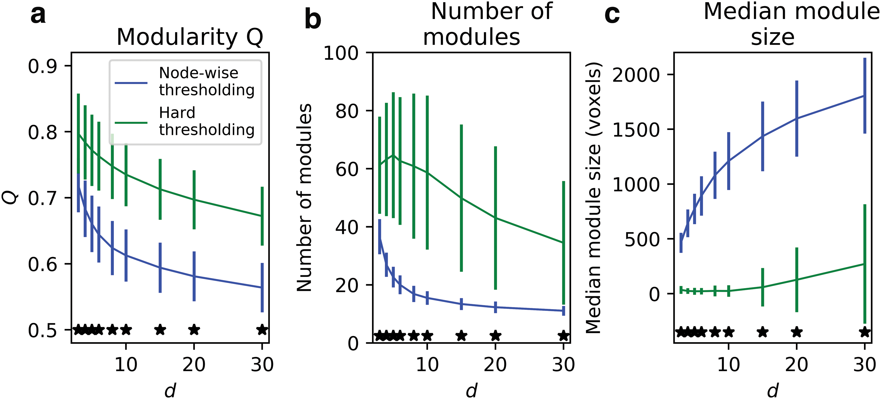
The mean and SD of various statistics associated with modular parcellation. The modularity Q (a), the number of modules (b), and the median module size (in voxels) (c) are plotted for hard thresholding networks and node-wise thresholding networks formed at different values of d. Significant differences between the two thresholding methods (paired t-test, p < 0.05, Bonferroni corrected) are indicated by stars. Color images available online at www.liebertpub.com/brain

Figure 6 illustrates differences in modular organization between hard thresholding and node-wise thresholding networks in a representative subject. Figure 6a shows relative module sizes as tree maps. In each tree map, the area of each rectangle represented the relative module size compared with the size of the giant component, represented as the collection of rectangles (Bruls et al., 2000). From the tree maps, it can be seen that the giant component was smaller than all the available nodes in hard thresholding networks, leaving many nodes fragmented from the giant component. Even within the giant component, the modular parcellation included a large number of small modules, as seen on the top right corner of each tree map. This was more apparent in networks formed with a small value of d. This demonstrated that even the giant component was fragmented into a large number of small modules in a hard thresholding network. On the contrary, there were no disconnected nodes in node-wise thresholding networks. Moreover, there were no extremely small modules comparable to fragmented micromodules seen in the hard thresholding network tree maps.

FIG. 6.

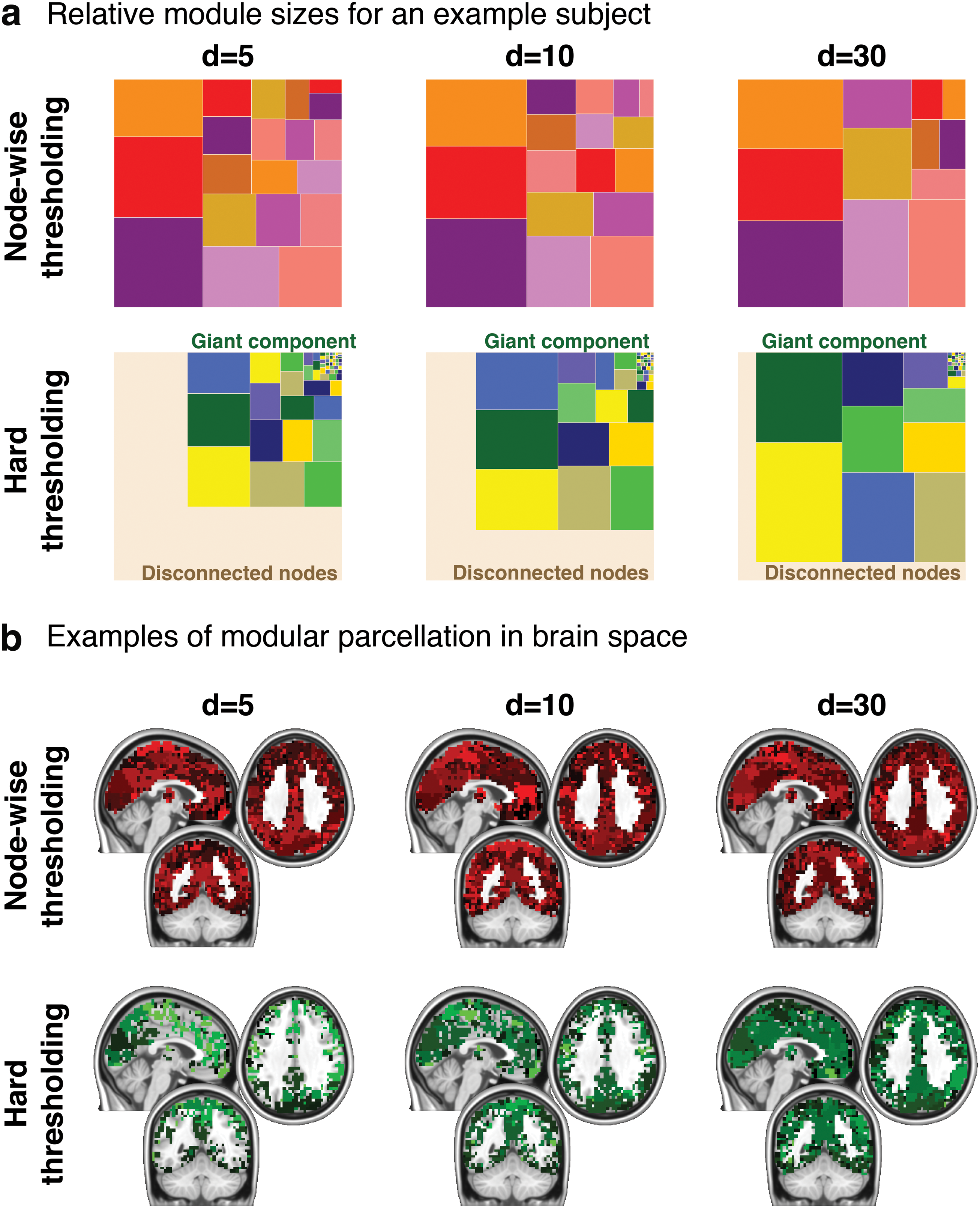
Examples of modular parcellation from a representative subject at d = 5, 10, and 30. (a) Relative module sizes are displayed as tree maps. The areas of rectangles correspond to relative module sizes compared to the giant component. The size of the giant component, as well as the collection of disconnected nodes, is also proportional to the availability of all nodes in hard thresholding networks. The colors of the rectangles are arbitrarily chosen to distinguish different modules. (b) Different modules are indicated by different colors in their locations in the brain space, overlaid on a template image. Due to a large number of disconnected components, there are holes in hard thresholding networks (b). Colors of modules are arbitrarily chosen to distinguish different modules. Color images available online at www.liebertpub.com/brain

In Figure 6a, disconnected components were not considered as modules and were displayed collectively at the bottom left of each tree map. A network module is defined as a collection of nodes that are highly interconnected among themselves and sparsely connected to the rest of nodes in the network. Disconnected components are fundamentally different from modules according to this definition, thus were not considered as network modules. The blank space at the bottom left shows how many of network nodes were disconnected.

Figure 6b shows modular parcellation in the brain space. Modules are shown with different arbitrary colors to show different modules. For node-wise thresholding networks, all available nodes were parcellated into different modules covering the gray matter areas in the cerebrum. On the contrary, for hard thresholding, modular parcellation images showed fragmented modules, with holes and missing voxels corresponding to disconnected nodes. Consequently, the gray matter cortical areas were not covered entirely, unlike the modular parcellation of node-wise thresholding networks. Even with d = 30, holes were still visible.

The fragmentation of modules seen in Figure 6 is based on one subject. To examine whether such fragmentation is a consistent phenomenon across subjects, the consistency of two known modules (DMN and SM modules) was examined (Fig. 7). Figure 7a shows the consistency of the DMN module. It can be seen that the DMN module was consistent for both thresholding methods and across different values of d, particularly in the precuneus and posterior cingulate cortex. This is not surprising since the DMN module likely coincides with areas of high-degree nodes (Fig. 4a). It is likely that such high-degree nodes are interconnected among themselves, forming the DMN module. Figure 7b shows the consistency of the SM module. The SM module was highly consistent in node-wise thresholding networks, regardless of the value of d. On the contrary, the SM module was consistent only for high d (d = 30) for hard thresholding networks. When d is small, modules, including the SM module, may be fragmented in hard thresholding networks, and this can lead to the lack of consistency across subjects, as seen in Figure 7b.

FIG. 7.

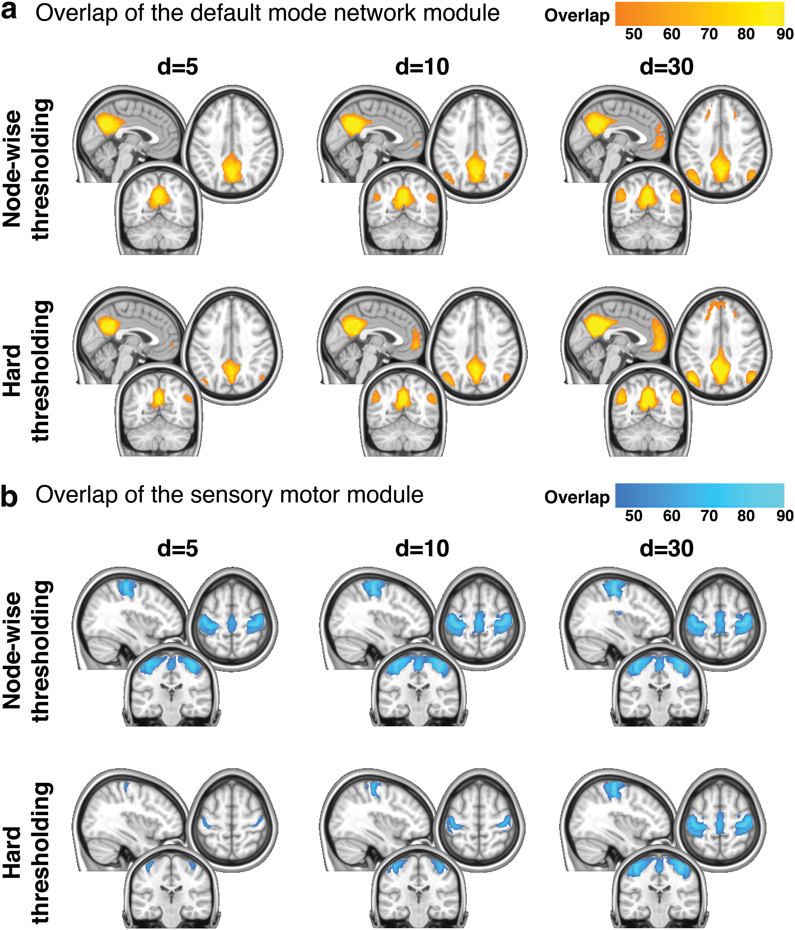
The consistency of the DMN module and the SM module across subjects. The overlap of the DMN module (a) and the SM module (b) across subjects was examined for different thresholding methods and d values. DMN, default mode network; SM, sensory motor. Color images available online at www.liebertpub.com/brain

Discussion

In this work, I have shown that networks formed with node-wise thresholding are less fragmented. In a node-wise thresholding network, the giant component included virtually all nodes even with a small value of d. On the contrary, hard thresholding networks included a large portion of disconnected nodes, especially when d is small. Even with a large value of d, voxel-based hard thresholding networks still included fragmented components. I have also shown that the modular organization of hard thresholding networks was also fragmented, including a large number of small modules. Such a fragmentation of modules was not observed in node-wise thresholding networks. Consequently, some of the modules, such as the SM module, are likely more robust in node-wise thresholding networks than hard thresholding networks.

Although both hard thresholding and node-wise thresholding networks were formed from the same correlation matrices, a node-wise thresholding network may be a more appropriate representation of the brain network as a whole. Unless the sparsity is high, a hard thresholding network likely includes disconnected nodes, and as it can be seen in Figure 6b, such fragmented nodes are located at seemingly random locations. In other words, the brain network is represented as a collection of disjoint networks; while the majority of nodes may be connected as the giant component, some parts of the brain are disconnected from the rest of the brain network. On the contrary, a node-wise thresholding network includes all available nodes, representing all brain nodes as part of a single network. As mentioned earlier, node-wise threshold networks undergo percolation, a system-wide phase-transition phenomenon in formation of a fully connected network (Hayasaka, 2016).

Although percolation is mentioned for hard thresholding networks in the literature (Alexander-Bloch et al., 2010; Fornito et al., 2012), no sign of percolation can be observed in hard thresholding networks, as it can be seen in Figure 2a and d, as well as in Hayasaka (2016). In node-wise thresholding networks, when new edges are added as d increases, edges are evenly distributed throughout the network in a way that does not alter the relative abundance of high- or low-degree nodes. In fact, the shape of degree distributions resembles with each other across different values of d (Fig. 3). On the contrary, in hard thresholding networks, the larger the d becomes, the more curved the degree distribution becomes, with edges unevenly concentrated in medium- to high-degree nodes. Larger clustering coefficient C seen in hard thresholding networks may be simply a manifestation of such concentration of edges. Although node-wise thresholding networks may have a smaller clustering coefficient C, they are more globally efficient with a smaller path length L.

Node-wise thresholding can be a great remedy for fragmented modules in hard thresholding. There are fewer yet larger modules in a node-wise thresholding network compared with the equivalent hard thresholding network. Such modules are robust and consistently observed across subjects, regardless of the value of d. On the contrary, some modules, such as the SM module, may be consistent only for a large value of d in hard thresholding networks. From these observations, one can conclude that the modular organization is more stable in node-wise thresholding than hard thresholding. One may argue that the modular organization can be examined in a hard thresholding network if d is sufficiently large, or equivalently the network has a sufficiently large number of edges. However, it is hard to determine what constitutes the adequate number of edges, since the modular organization is highly dependent on it.

There is no clear consensus in the field as to what threshold or sparsity should be used to form a functional connectivity network. In fact, people often use a range of thresholds and examine network characteristics over that range [see Fornito et al. (2013) for a review]. The rationale for using multiple thresholds is that network characteristics are dependent on the threshold. This is likely true for hard thresholding networks, but for node-wise thresholding, especially for voxel-based networks, the relative giant component size G or the clustering coefficient C does not vary across different values of d. Only the path length L shortens as d increases. Although modular organization statistics, such as the modularity Q or the median module size, may change over different values of d in node-wise thresholding networks, key modules such as the DMN and SM modules are robust regardless of the value of d.

Thus, in my opinion, examining multiple node-wise thresholding networks formed at different values of d may not be necessary. The information ascertained from a network formed at a particular value of d can be likely replicated in a network formed at a different value of d. For voxel-based networks, any d ≥ 5 would be adequate. Based on the network density formula for self-organized networks by Laurienti et al. (2011), the average degree of a network with M = 19,000 nodes should be M × 7.89 M ^−0.986 = 9.06. Thus, I recommend d = 10 to ensure that the average degree is at least 10. One can use a larger value of d, but that involves more edges in a network and consequently that may slow down various computationally intensive analysis procedures, such as path length calculation or modular parcellation.

Although node-wise thresholding can address some shortcomings of hard thresholding, there are some limitations. First, node-wise thresholding forces each node to have a certain number of connections, dictated by d. This means that, if there are truly disconnected nodes, such nodes may be erroneously included in a network. Second, correlation coefficients associated with some edges may be considerably small. This can be seen as inclusion of weak connections to a network. Individually, such weak connections may appear unrealistic, especially when compared to high correlation coefficients in a correlation matrix. However, such weak connections may play a crucial role in forming a network together, connecting otherwise disconnected components to the main network (Foti et al., 2011).

There is an alternative way to construct nonfragmented networks with hard thresholding. This is done by lowering the threshold sufficiently so that almost all (e.g., 99%) nodes are connected as a giant component (Bassett et al., 2006; van Wijk et al., 2010). Although the resulting network may not contain a large number of disconnected components, it still suffers from the same shortcomings of hard thresholding networks.

To demonstrate this point, I performed an additional analysis of hard thresholded networks whose 99% or more nodes were connected to the giant component. The degree distribution (shown in Fig. 8) was similar to the degree distributions of hard thresholding networks with high d, suggesting relative abundance of medium- to high-degree nodes. Fragmentation of network modules was also observed. Of networks generated from n = 123 subjects, 84.6% of them contained at least one extremely small module (consisting of ≤20 nodes, or ∼0.1% of nodes). Of those, 84.6% of networks were with extremely small modules, on average 31.1% of modules were extremely small modules. This suggests that fragmentation of network modules cannot be prevented simply by lowering the threshold in hard thresholding.

FIG. 8.

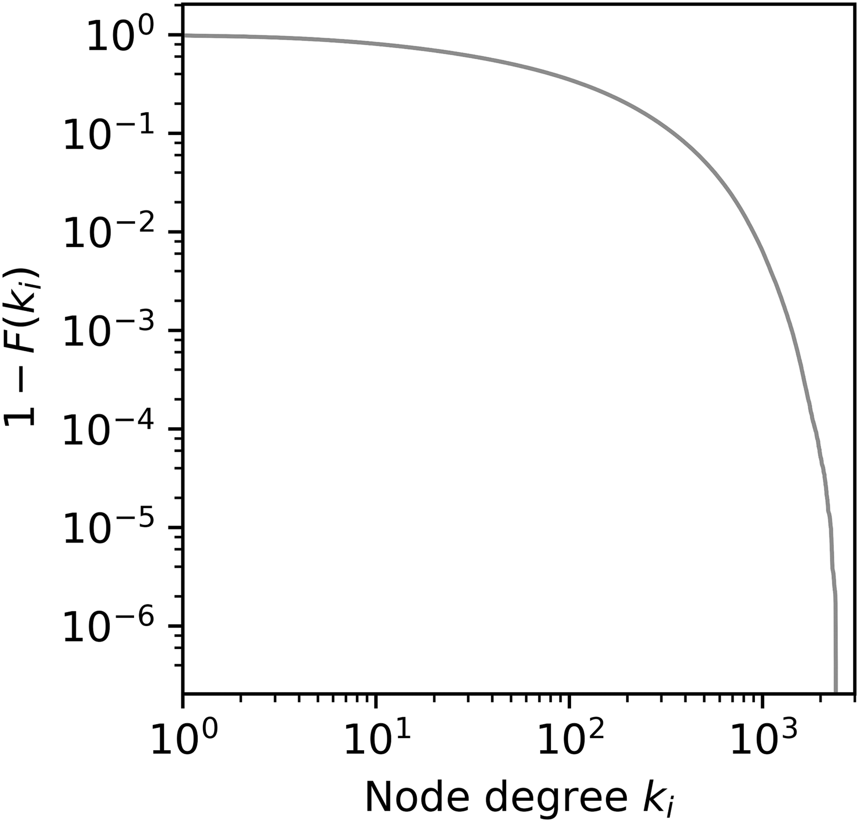
Degree distribution of voxel-based hard thresholding networks with 99% of nodes connected to the giant component. The degree distribution is a combined distribution of n = 123 networks.

Conclusion

In this work, I applied an alternative thresholding approach, node-wise thresholding, to construct a functional connectivity network derived from a correlation matrix. I demonstrated that the network generated from this alternative method is robust against fragmentation in a network resulting from hard thresholding: fragmentation manifesting as disconnected nodes and fragmentation manifesting as a large number of small modules. This anti-fragmentation property resulted in networks with highly consistent modules, regardless of the threshold. Moreover, edges are evenly distributed in node-wise thresholding networks without altering the relative abundance of low- or high-degree nodes. This is in contrast to hard thresholding where edges tend to concentrate in medium- to high-degree nodes as new edges are introduced. In conclusion, considering all these points, I believe that the functional connectivity of the brain as a single system can be more appropriately represented in a node-wise thresholding network.

Footnotes

Acknowledgment

This work was supported, in part, by the National Institute of Neurological Disorders and Stroke (NINDS; R01-NS070917).

Author Disclosure Statement

No competing financial interests exist.

References

Alexander-Bloch

, Gogtay

, Meunier

, Birn

, Clasen

, Lalonde

, et al. 2010. Disrupted modularity and local connectivity of brain functional networks in childhood-onset schizophrenia. Front Syst Neurosci, 4:147.

Barabasi

, Albert

. 1999. Emergence of scaling in random networks. Science, 286:509–512.

Bassett

, Meyer-Lindenberg

, Achard

, Duke

, Bullmore

. 2006. Adaptive reconfiguration of fractal small-world human brain functional networks. Proc Natl Acad Sci U S A, 103:19518–19523.

Biswal

, Yetkin

, Haughton

, Hyde

. 1995. Functional connectivity in the motor cortex of resting human brain using echo-planar MRI. Magn Reson Med, 34:537–541.

Blondel

, Guillaume

, Lambiotte

, Lefebvre

. 2008. Fast unfolding of communities in large networks. J Stat Mech, 2008:P10008.

Borchers

, Himmelbach

, Logothetis

, Karnath

. 2011. Direct electrical stimulation of human cortex—the gold standard for mapping brain functions?. Nat Rev Neurosci, 13:63–70.

Bruls

, Huizing

, van Wijk

. 2000. Squarified treemaps. Spring Comp Sci, 2000:33–42.

Fornito

, Zalesky

, Breakspear

. 2013. Graph analysis of the human connectome: promise, progress, and pitfalls. Neuroimage, 80:426–444.

Fornito

, Zalesky

, Bullmore

. 2010. Network scaling effects in graph analytic studies of human resting-state FMRI data. Front Syst Neurosci, 4:22.

10.

Fornito

, Zalesky

, Pantelis

, Bullmore

. 2012. Schizophrenia, neuroimaging and connectomics. Neuroimage, 62:2296–2314.

11.

Foti

, Hughes

, Rockmore

. 2011. Nonparametric sparsification of complex multiscale networks. PLoS One, 6:e16431.

12.

Fox

, Snyder

, Vincent

, Corbetta

, Van Essen

, Raichle

. 2005. The human brain is intrinsically organized into dynamic, anticorrelated functional networks. Proc Natl Acad Sci U S A, 102:9673–9678.

13.

Hayasaka

. 2013. Functional connectivity networks with and without global signal correction. Front Hum Neurosci, 7:880.

14.

Hayasaka

. 2016. Explosive percolation in thresholded networks. Phys A Stat Mech Appl, 451:1–9.

15.

Hayasaka

, Laurienti

. 2010. Comparison of characteristics between region-and voxel-based network analyses in resting-state fMRI data. Neuroimage, 50:499–508.

16.

Jenkinson

, Beckmann

, Behrens

, Woolrich

, Smith

. 2012. FSL. Neuroimage, 62:782–790.

17.

Laurienti

, Joyce

, Telesford

, Burdette

, Hayasaka

. 2011. Universal fractal scaling of self-organized networks. Phys A, 390:3608–3613.

18.

Moussa

, Vechlekar

, Burdette

, Steen

, Hugenschmidt

, Laurienti

. 2011. Changes in cognitive state alter human functional brain networks. Front Hum Neurosci, 5:83.

19.

Newman

. 2006a. Finding community structure in networks using the eigenvectors of matrices. Phys Rev E Stat Nonlin Soft Matter Phys, 74(3 Pt 2):036104.

20.

Newman

. 2006b. Modularity and community structure in networks. Proc Natl Acad Sci U S A, 103:8577–8582.

21.

Newman

, Girvan

. 2004. Finding and evaluating community structure in networks. Phys Rev E Stat Nonlin Soft Matter Phys, 69(2 Pt 2):026113.

22.

Power

, Barnes

, Snyder

, Schlaggar

, Petersen

. 2012. Spurious but systematic correlations in functional connectivity MRI networks arise from subject motion. Neuroimage, 59:2142–2154.

23.

Power

, Cohen

, Nelson

, Wig

, Barnes

, Church

, et al. 2011. Functional network organization of the human brain. Neuron, 72:665–678.

24.

Raichle

, Snyder

. 2007. A default mode of brain function: a brief history of an evolving idea. Neuroimage, 37:1083–1090; discussion 1097–1089.

25.

Ruan

, Dean

, Zhang

. 2010. A general co-expression network-based approach to gene expression analysis: comparison and applications. BMC Syst Biol, 4:8.

26.

Rubinov

, Sporns

. 2010. Complex network measures of brain connectivity: uses and interpretations. Neuroimage, 52:1059–1069.

27.

Smith

, Jenkinson

, Woolrich

, Beckmann

, Behrens

, Johansen-Berg

, et al. 2004. Advances in functional and structural MR image analysis and implementation as FSL. Neuroimage, 23 Suppl 1:S208–219.

28.

Stam

, Reijneveld

. 2007. Graph theoretical analysis of complex networks in the brain. Nonlinear Biomed Phys, 1:3.

29.

Tzourio-Mazoyer

, Landeau

, Papathanassiou

, Crivello

, Etard

, Delcroix

, et al. 2002. Automated anatomical labeling of activations in SPM using a macroscopic anatomical parcellation of the MNI MRI single-subject brain. Neuroimage, 15:273–289.

30.

van den Heuvel

, Stam

, Boersma

, Hulshoff Pol

. 2008. Small-world and scale-free organization of voxel-based resting-state functional connectivity in the human brain. Neuroimage, 43:528–539.

31.

Van Dijk

, Hedden

, Venkataraman

, Evans

, Lazar

, Buckner

. 2010. Intrinsic functional connectivity as a tool for human connectomics: theory, properties, and optimization. J Neurophysiol, 103:297–321.

32.

van Wijk

, Stam

, Daffertshofer

. 2010. Comparing brain networks of different size and connectivity density using graph theory. PLoS One, 5:e13701.

33.

Wang

, Wang

, Zang

, Yang

, Tang

, Gong

, et al. 2009. Parcellation-dependent small-world brain functional networks: a resting-state fMRI study. Hum Brain Mapp, 30:1511–1523.

34.

Worsley

, Cao

, Paus

, Petrides

, Evans

. 1998. Applications of random field theory to functional connectivity. Hum Brain Mapp, 6:364–367.