On the Origin of Individual Functional Connectivity Variability: The Role of White Matter Architecture

Abstract

Fingerprint patterns derived from functional connectivity (FC) can be used to identify subjects across groups and sessions, indicating that the topology of the brain substantially differs between individuals. However, the source of FC variability inferred from resting-state functional magnetic resonance imaging remains unclear. One possibility is that these variations are related to individual differences in white matter structural connectivity (SC). However, directly comparing FC with SC is challenging given the many potential biases associated with quantifying their respective strengths. In an attempt to circumvent this, we employed a recently proposed test–retest approach that better quantifies inter-subject variability by first correcting for intra-subject nuisance variability (i.e., head motion, physiological differences in brain state, etc.) that can artificially influence FC and SC measures. Therefore, rather than directly comparing the strength of FC with SC, we asked whether brain regions with, for example, low inter-subject FC variability also exhibited low SC variability. From this, we report two main findings: First, at the whole-brain level, SC variability was significantly lower than FC variability, indicating that an individual's structural connectome is far more similar to another relative to their functional counterpart even after correcting for noise. Second, although FC and SC variability were mutually low in some brain areas (e.g., primary somatosensory cortex) and high in others (e.g., memory and language areas), the two were not significantly correlated across all cortical and sub-cortical regions. Taken together, these results indicate that even after correcting for factors that may differently affect FC and SC, the two, nonetheless, remain largely independent of one another. Further work is needed to understand the role that direct anatomical pathways play in supporting vascular-based measures of FC and to what extent these measures are dictated by anatomical connectivity.

Introduction

Each brain is uniquely organized, both functionally (Wang and Liu, 2014) and structurally (Lange et al., 1997). The cerebral architecture is known to evolve across time due to brain development and plasticity (Poldrack et al., 2015; Wierenga et al., 2016), and the complexity of these changes during development is often reflected by regional differences across subjects. These so-called inter-individual differences in brain function and structure are of great interest as they allow researchers to directly compare how these cerebral differences correlate with other measures such as—among others—musical (Gaser and Schlaug, 2003) and athletic (Yarrow et al., 2009) ability.

Recently, two magnetic resonance imaging (MRI)-based methodologies have emerged as non-invasive measures of the brain's functional connectivity (FC) and structural connectivity (SC). Functional MRI (fMRI) provides four-dimensional whole-brain images that reflect changes in cortical blood flow, volume, and oxygen as measured by the blood-oxygenation-level-dependent (BOLD) signal (Bandettini et al., 1993; Kwong et al., 1992; Turner, 1992). At rest, the spontaneous low-frequency fluctuations (<0.08–0.1 Hz) in the BOLD signal allow the detection of temporally correlated spatial patterns that are specific to each individual (Biswal et al., 1995; Damoiseaux et al., 2006) and are generally believed to reflect neuronal synchronization between brain areas [see Buckner et al. (2013) and references therein]. Diffusion MRI (dMRI), on the other hand, provides information about the structural architecture of the brain by probing the diffusion of water molecules in the white matter (WM) and is often used to infer anatomical or SC between brain regions.

It is well established that the strength of BOLD FC (often expressed as a correlation coefficient or z-score) varies across healthy individuals, though the source of this variability is unclear. Several studies have suggested that the “strength” or “integrity” of direct anatomical pathways between brain areas is related to the strength of their FC (Bowman et al., 2012; Goni et al., 2014; Hermundstad et al., 2013; Honey et al., 2009; Sporns, 2013; van den Heuvel et al., 2009; Varkuti et al., 2011; Ward et al., 2014; Zhu et al., 2014). However, other studies have reported a poor correlation between the two. For instance, FC is barely altered in patients with aggressive brain tumors (Ghumman et al., 2016), despite the fact that such insults can dramatically alter SC (Fornito et al., 2015; Leclercq et al., 2011; Nimsky et al., 2005, 2016). Similarly, individuals with complete agenesis of the corpus callosum (CC), nonetheless, display intact bilateral FC (Tyszka et al., 2011), demonstrating that FC between two brain areas is not necessarily dependent on a direct anatomical connection (Buckner et al., 2013).

It is also well established that BOLD FC varies more across subjects than repeated measures within the same subject (Finn et al., 2015), and Mueller and associates (2013) were the first groups to explicitly demonstrate that functional inter-subject variability \documentclass{aastex}\usepackage{amsbsy}\usepackage{amsfonts}\usepackage{amssymb}\usepackage{bm}\usepackage{mathrsfs}\usepackage{pifont}\usepackage{stmaryrd}\usepackage{textcomp}\usepackage{portland, xspace}\usepackage{amsmath, amsxtra}\usepackage{upgreek}\pagestyle{empty}\DeclareMathSizes{10}{9}{7}{6}\begin{document}$${ \rm{ ( \bf V}}_{inter}^{FC} )$$ \end{document} is heterogeneously distributed across the whole brain. Specifically, their results indicated that the association cortex shows higher signs of variability, whereas the motor and visual networks shows low variance across individuals. A distinguishing point of their study is that these results were achieved by taking into account the intra-subject variability of each individual. The major advantage of this approach is that since intra-subject variability represents measurement noise that cannot be estimated in a single scanning session, regressing it from inter-subject variability measures ensures that these measures cannot be explained by scanner noise, temporal changes in signal to noise ratio (SNR), head motion, brain state, and other confounding factors, all of which are known to affect FC in single subjects (Murphy et al., 2013). Importantly, some of these factors, as well as others also affect measures of SC. Indeed, studying SC can be difficult given the numerous confounding factors (e.g., false positives, seeding method, stopping criteria, label size, etc.) (Bastiani et al., 2012; Colon-Perez et al., 2015; Girard et al., 2014; Jones et al., 2013; Maier-Hein et al., 2016; Zalesky et al., 2016) that are typically insignificant in FC analysis. Existing structural connectome reproducibility studies often rely on a single value to quantify variability across the whole brain or across the whole connectivity matrix (e.g., global network metrics) (Cammoun et al., 2012; Cheng et al., 2012; Owen et al., 2013), and as a result, is highly unspecific for each brain region (Smith et al., 2015). Moreover, common network analysis often only employs cortical regions, and thus, neglects the inclusion of sub-cortical nuclei (e.g., thamalus) (Cheng et al., 2012; Gong et al., 2009; Hagmann et al., 2007). Omitting these regions implies that large WM fascicles connecting these nuclei to the cortex (e.g., thalamo-cortical projections) are completely discarded from the network analysis. Particularly, overlooking the brainstem in network construction often means that streamlines forming the corticospinal tract (CST) are also absent from the resulting SC matrix. Therefore, given the problems associated with directly comparing the strength of FC with that of SC, the method proposed by Mueller and colleagues (2013) offers a new approach for comparing FC and SC by directly comparing their variability. That is, can we assume that a given brain area displaying low \documentclass{aastex}\usepackage{amsbsy}\usepackage{amsfonts}\usepackage{amssymb}\usepackage{bm}\usepackage{mathrsfs}\usepackage{pifont}\usepackage{stmaryrd}\usepackage{textcomp}\usepackage{portland, xspace}\usepackage{amsmath, amsxtra}\usepackage{upgreek}\pagestyle{empty}\DeclareMathSizes{10}{9}{7}{6}\begin{document}$${ \rm{\bf V}}_{inter}^{FC}$$ \end{document} also shows low structural inter-subject variability ( \documentclass{aastex}\usepackage{amsbsy}\usepackage{amsfonts}\usepackage{amssymb}\usepackage{bm}\usepackage{mathrsfs}\usepackage{pifont}\usepackage{stmaryrd}\usepackage{textcomp}\usepackage{portland, xspace}\usepackage{amsmath, amsxtra}\usepackage{upgreek}\pagestyle{empty}\DeclareMathSizes{10}{9}{7}{6}\begin{document}$${ \bf V}_{inter}^{SC}$$ \end{document} )?

To investigate to what extent variations in SC are related to FC variability, we applied the approach proposed by Mueller and colleagues (2013) (originally intended for mapping functional variability) on SC matrices derived from dMRI tractography initiated from the WM and gray matter (GM) interface. The resulting structural variability indices were then compared with functional variability maps to determine whether those variances are predictive of one another. Using this approach, we report whole-brain SC variability measures that take into account the aforementioned biases and compare them with FC variability. We globally determined that structural variability is lower than functional variability. We also observed that regions of low (i.e., motor areas) and high (i.e., memory and language areas) functional variability also exhibited signs of low and high structural variability, respectively. Finally, our results suggest that the bulk of inter-individual variability in FC cannot be explained by corresponding variability in SC.

Methods

Anatomical, diffusion, and functional datasets were obtained on a 1.5 T Siemens Magnetom from nine subjects (s) over three sessions (t) separated by a 1 month interval (seven men; mean age 25 years ±3.1; range 21–30). An additional functional dataset was acquired during the last session for all participants. The study was performed according to the guidelines of the Internal Review Board of the Centre Hospitalier Universitaire de Sherbrooke. Acquisition details and processing steps are illustrated in Figure 1 and described later.

FIG. 1.

SC and FC pipeline. Brain parcellation was first performed on each subject-specific anatomical images, resulting in 159 cortical and subcortical regions. Top: FC matrices were generated by averaging the preprocessed signals within each of the brain regions and correlating them between each other. FC matrices were group-normalized by applying Fisher's r-to-z transform. Bottom: Probabilistic streamline tractography was done by using particle filtering tractography (Girard et al., 2014) with dense seeding from the white matter and gray matter interface (10 seeds/voxel). SC matrices were generated by computing the connectivity between pairs of cortical regions and normalized to account for various total streamline counts. FC, functional connectivity; SC, structural connectivity. Color images available online at www.liebertpub.com/brain

Structural connectivity

High angular resolution diffusion imaging (HARDI) data were acquired along 64 uniformly distributed directions by using a b-value of 1000 sec/mm², a single-shot echo-planar imaging (EPI) sequence (128 × 128 matrix, 2 mm isotropic resolution, TR/TE 11,000/98 msec), and a GRAPPA factor of 2. The diffusion-weighted data of each subject were upsampled to the anatomical resolution (1 mm isotropic). Partial volume estimation (PVE) maps were obtained from the T1-weighted image (1 mm isotropic MPRAGE, TR/TE 6.57/2.52 msec) by using FSL-Fast (Zhang et al., 2001) and registered to the upsampled diffusion-weighted images. PVE were used in the particle filtering tractography algorithm by using anatomical priors (Girard et al., 2014) to provide a better tracking domain as opposed to fractional anisotropy-based mask, where streamline propagation is often prematurely halted in crossing regions (Descoteaux, 2015; Girard et al., 2014; Nimsky et al., 2016; Seunarine and Alexander, 2009; Smith et al., 2012). Fiber orientation distribution functions were obtained from constrained spherical deconvolution (Tournier et al., 2007, 2012), with a spherical harmonic order of 8. Probabilistic streamline tractography was done by using particle filtering tractography (Girard et al., 2014), seeding from the WM/GM interface (Girard et al., 2014; Smith et al., 2012) using 10 seeds per voxel (∼2,000,000 seeds leading to 1,400,000 surviving streamlines). The particle filtering tractography algorithm ensured that streamlines did not terminate prematurely in the WM by the application of a back-tracking rule to allow the tractography algorithm to find alternative pathways. Freesurfer (Fischl et al., 2004) was used to obtain a brain parcellation of 159 regions [Destrieux et al. (2010), see Supplementary Data for label description; Supplementary Data are available online at www.liebertpub.com/brain] for each individual anatomical T1-weighted image. Subcortical regions were included to ensure an accurate representation of WM connections throughout the brain (e.g., thalamocortical radiations). The same reasoning was applied to the brain stem and cerebellum regions for the inclusion of corticospinal/corticocerebellar tracts. SC matrices (M_{n × n}) (Hagmann et al., 2007) were defined as the number of streamlines connecting pairs of cortical regions and computed by using Dipy (Garyfallidis et al., 2014) The M matrices were then normalized to account for various total streamline counts across different subjects, such that: \documentclass{aastex}\usepackage{amsbsy}\usepackage{amsfonts}\usepackage{amssymb}\usepackage{bm}\usepackage{mathrsfs}\usepackage{pifont}\usepackage{stmaryrd}\usepackage{textcomp}\usepackage{portland, xspace}\usepackage{amsmath, amsxtra}\usepackage{upgreek}\pagestyle{empty}\DeclareMathSizes{10}{9}{7}{6}\begin{document} \begin{align*} \mathop \sum \limits_{i , j} {\, \rm{ M}} = 1 , \end{align*} \end{document}

where i, j, ∈ lower diagonal of M (Girard et al., 2015) SC matrices were finally row-normalized to account for differences in streamline count within each brain region, according to: \documentclass{aastex}\usepackage{amsbsy}\usepackage{amsfonts}\usepackage{amssymb}\usepackage{bm}\usepackage{mathrsfs}\usepackage{pifont}\usepackage{stmaryrd}\usepackage{textcomp}\usepackage{portland, xspace}\usepackage{amsmath, amsxtra}\usepackage{upgreek}\pagestyle{empty}\DeclareMathSizes{10}{9}{7}{6}\begin{document} \begin{align*} \mathop \sum \limits_{i = 1}^n { \rm{ }}{{ \rm{M}}_{ij}} = 1 , \forall j = 1 \;:\; n. \end{align*} \end{document}

The result is a probability distribution function that expresses the probability of region A to be connected with all other regions (Ghaziri et al., 2017).

Functional connectivity

Continuous functional recordings were carried out by using a standard EPI sequence (eyes closed). For each run, 108 functional volumes consisting of 35 axial slices were obtained with a 64 × 64 matrix, field of view 220 mm, TR/TE 2730/40 msec, for a voxel size of 3.4 × 3.4 × 4.2 mm³. Preprocessing steps were performed in AFNI (Cox, 1996) and consisted of slice timing and motion correction, spatial smoothing based on non-local means (NLM) denoising (Bernier et al., 2014; Coupe et al., 2008), and band-pass temporal filtering (0.008–0.1 Hz). The use of NLM denoising allowed an improved identification of the BOLD signal in subcortical areas at 1.5 T, thus permitting a better comparison with diffusion data. Preprocessed signals were averaged within each of the aforementioned 159 regions (see Supplementary Data) after upsampling to the T1-space. Finally, the connectivity between each possible pair was assessed by computing their mutual covariance using Pearson's product-moment correlation. Finally, these correlation coefficients were converted to z-scores by using Fisher's r-to-z transform for standardization across subjects.

Inter-subject variability

Variability indices were computed by using the approach proposed by Mueller and associates (2013). The outline of the method is described as follows and was repeated for both FC and SC matrices: For each of the 159 brain regions, an inter-subject variability index (V_inter) was derived by regression of the intra-subject variability from an estimated group-variance index. Methodological details describing the estimations of variability indices are given later and are illustrated in Figure 2.

• Group similarity (Sim ^t): For each session t, the similarity between homologous region (i.e., corresponding rows of connectivity matrices) is given by the correlation (r) of those two connectivity profiles, averaged across subjects (Fig. 2, step 1).

• Intra-subject variability (V _intra): The across-session variability (1-similarity) between homologous regions was first estimated for each subject s (Fig. 2, step 2). \documentclass{aastex}\usepackage{amsbsy}\usepackage{amsfonts}\usepackage{amssymb}\usepackage{bm}\usepackage{mathrsfs}\usepackage{pifont}\usepackage{stmaryrd}\usepackage{textcomp}\usepackage{portland, xspace}\usepackage{amsmath, amsxtra}\usepackage{upgreek}\pagestyle{empty}\DeclareMathSizes{10}{9}{7}{6}\begin{document}$${ \bf V}_{intra}^{ \rm{s}}$$ \end{document} values were then averaged across all subjects, resulting in a single value (V _intra) for each brain region (Fig. 2, step 3).

• Inter-subject variability (V _inter): For each session t, linear least-squares regression allowed the estimation of the inter-subject variability, given by \documentclass{aastex}\usepackage{amsbsy}\usepackage{amsfonts}\usepackage{amssymb}\usepackage{bm}\usepackage{mathrsfs}\usepackage{pifont}\usepackage{stmaryrd}\usepackage{textcomp}\usepackage{portland, xspace}\usepackage{amsmath, amsxtra}\usepackage{upgreek}\pagestyle{empty}\DeclareMathSizes{10}{9}{7}{6}\begin{document}$${ \bf V}_{inter}^t$$ \end{document} = [1 − Sim ^t] − β V _intra − c (Fig. 2, step 4). A single value (V _inter) was finally obtained for each region by averaging the residual maps ( \documentclass{aastex}\usepackage{amsbsy}\usepackage{amsfonts}\usepackage{amssymb}\usepackage{bm}\usepackage{mathrsfs}\usepackage{pifont}\usepackage{stmaryrd}\usepackage{textcomp}\usepackage{portland, xspace}\usepackage{amsmath, amsxtra}\usepackage{upgreek}\pagestyle{empty}\DeclareMathSizes{10}{9}{7}{6}\begin{document}$${ \bf V}_{inter}^t$$ \end{document} ) over all sessions (Fig. 2, step 5).

FIG. 2.

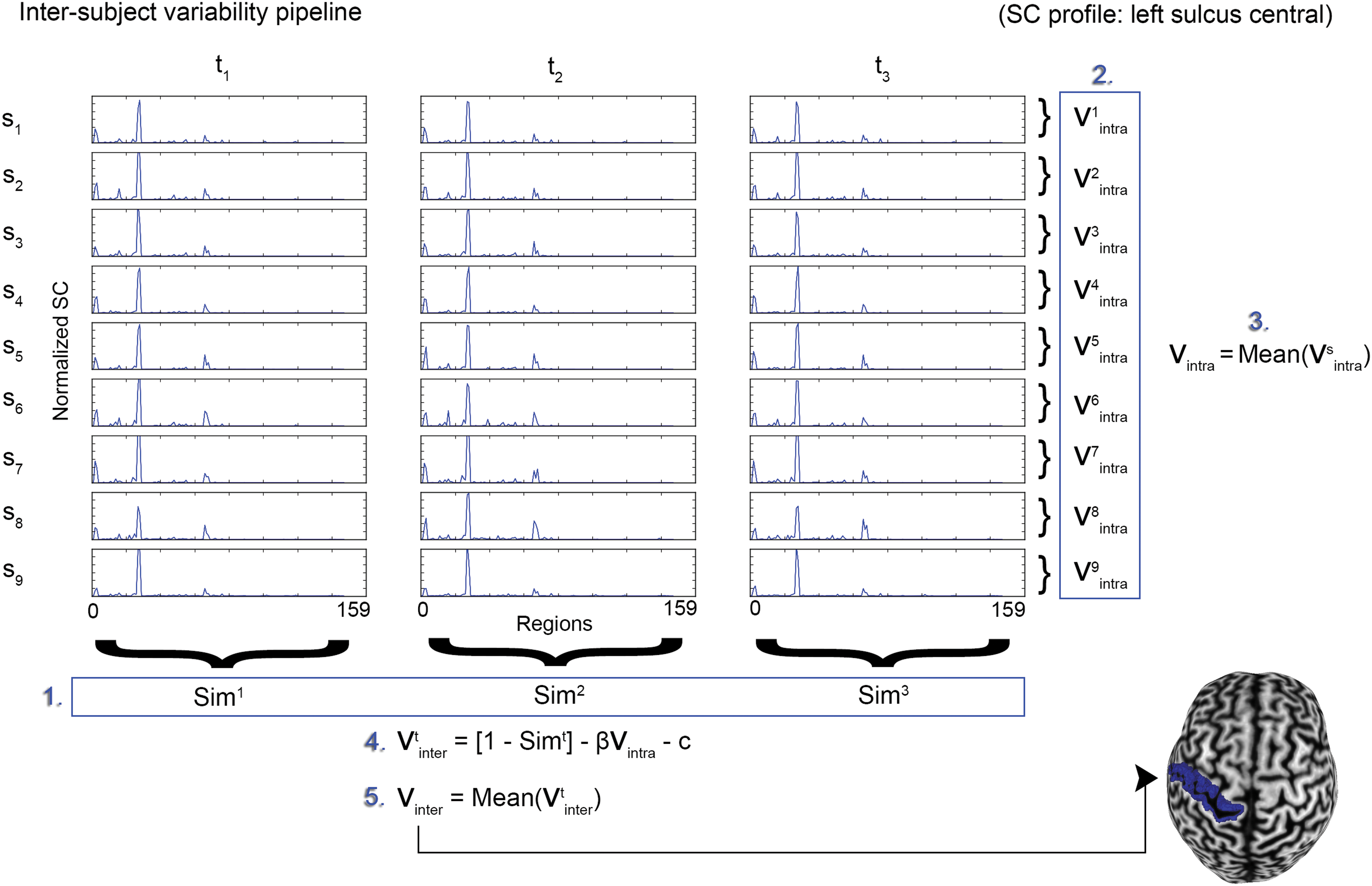
Inter-subject variability pipeline illustrated for a single brain region (left central sulcus, SC profile). Starting with s subjects and t sessions, the similarity between subjects was estimated for each session t by averaging the correlations between corresponding brain regions (1). Next (2), the across session variability was estimated for each subject s by averaging the correlation between homologous regions and subtracting from (1). Intra-subject variability values were then averaged across all subjects (3). Inter-subject variability was estimated for each session by t using ordinary least-squares regression (4), and it was finally averaged to obtain a single value for each region (5). The resulting indices were then back-projected to a brain surface for visualization. The pipeline was repeated independently for both FC and SC matrices. Color images available online at www.liebertpub.com/brain

With tractography, larger regions may be overly connected as opposed to regions with a lower volume or surface area. Thus, to exclude any confounding factors potentially related to volume differences across the 159 regions, \documentclass{aastex}\usepackage{amsbsy}\usepackage{amsfonts}\usepackage{amssymb}\usepackage{bm}\usepackage{mathrsfs}\usepackage{pifont}\usepackage{stmaryrd}\usepackage{textcomp}\usepackage{portland, xspace}\usepackage{amsmath, amsxtra}\usepackage{upgreek}\pagestyle{empty}\DeclareMathSizes{10}{9}{7}{6}\begin{document}$${ \bf V}_{inter}^{SC}$$ \end{document} values were corrected by the average seeding surface area (mm²) by using ordinary least-squares regression. Specifically, the seeding surface area of a region was defined as the number of voxels of the WM/GM interface intersecting with that region (Supplementary Fig. S1) and averaged across subjects.

Subsequently, structural and functional V_inter indices were back-projected to a brain surface for better spatial characterization. Statistical analysis included a direct comparison of functional and structural variability scores using Pearson's product-moment correlation. Finally, mutual regions of low and high variability were determined by isolating regions located in the top and bottom 15% (z = 1) of \documentclass{aastex}\usepackage{amsbsy}\usepackage{amsfonts}\usepackage{amssymb}\usepackage{bm}\usepackage{mathrsfs}\usepackage{pifont}\usepackage{stmaryrd}\usepackage{textcomp}\usepackage{portland, xspace}\usepackage{amsmath, amsxtra}\usepackage{upgreek}\pagestyle{empty}\DeclareMathSizes{10}{9}{7}{6}\begin{document}$${ \bf V}_{inter}^{FC}$$ \end{document} and \documentclass{aastex}\usepackage{amsbsy}\usepackage{amsfonts}\usepackage{amssymb}\usepackage{bm}\usepackage{mathrsfs}\usepackage{pifont}\usepackage{stmaryrd}\usepackage{textcomp}\usepackage{portland, xspace}\usepackage{amsmath, amsxtra}\usepackage{upgreek}\pagestyle{empty}\DeclareMathSizes{10}{9}{7}{6}\begin{document}$${ \bf V}_{inter}^{SC}$$ \end{document} . This threshold was empirically determined by looking at the shape of the sorted variability scores for both FC and SC analysis.

Results

Functional variability

Whole-brain \documentclass{aastex}\usepackage{amsbsy}\usepackage{amsfonts}\usepackage{amssymb}\usepackage{bm}\usepackage{mathrsfs}\usepackage{pifont}\usepackage{stmaryrd}\usepackage{textcomp}\usepackage{portland, xspace}\usepackage{amsmath, amsxtra}\usepackage{upgreek}\pagestyle{empty}\DeclareMathSizes{10}{9}{7}{6}\begin{document}$${ \bf V}_{inter}^{FC}$$ \end{document} indices are illustrated in Figure 3 (left). Low variability was found near the motor and visual areas (Fig. 3, black arrowheads), showing strong correspondence with previous functional analysis work from Mueller and colleagues (2013) (top left subfigure). Conversely, high variability is also present across the left (l) and right (r) temporal lobes, as well as near the language areas. In addition to the previous spatial maps, Figure 4 (top) shows a quantitative indexing of \documentclass{aastex}\usepackage{amsbsy}\usepackage{amsfonts}\usepackage{amssymb}\usepackage{bm}\usepackage{mathrsfs}\usepackage{pifont}\usepackage{stmaryrd}\usepackage{textcomp}\usepackage{portland, xspace}\usepackage{amsmath, amsxtra}\usepackage{upgreek}\pagestyle{empty}\DeclareMathSizes{10}{9}{7}{6}\begin{document}$${ \bf V}_{inter}^{FC}$$ \end{document} for each of the 159 regions (red). The mean functional variance derived from all brain regions was 0.25 ± 0.04 (red dotted lines) with \documentclass{aastex}\usepackage{amsbsy}\usepackage{amsfonts}\usepackage{amssymb}\usepackage{bm}\usepackage{mathrsfs}\usepackage{pifont}\usepackage{stmaryrd}\usepackage{textcomp}\usepackage{portland, xspace}\usepackage{amsmath, amsxtra}\usepackage{upgreek}\pagestyle{empty}\DeclareMathSizes{10}{9}{7}{6}\begin{document}$${ \bf V}_{intra}^{FC}$$ \end{document} of 0.41 ± 0.12 (uncorrected mean \documentclass{aastex}\usepackage{amsbsy}\usepackage{amsfonts}\usepackage{amssymb}\usepackage{bm}\usepackage{mathrsfs}\usepackage{pifont}\usepackage{stmaryrd}\usepackage{textcomp}\usepackage{portland, xspace}\usepackage{amsmath, amsxtra}\usepackage{upgreek}\pagestyle{empty}\DeclareMathSizes{10}{9}{7}{6}\begin{document}$${ \bf V}_{inter}^{FC}$$ \end{document} was 0.55 ± 0.12).

FIG. 3.

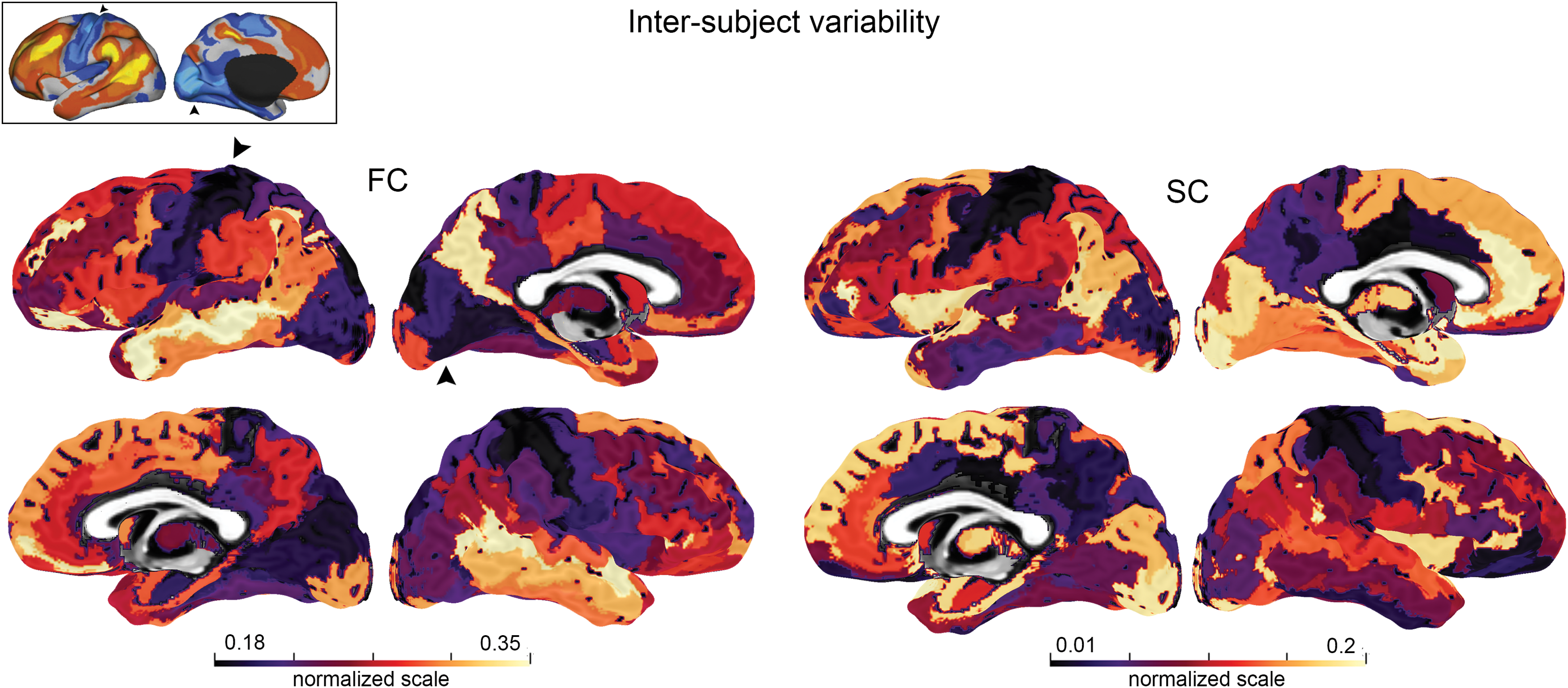
Normalized functional and structural inter-subject variability maps back-projected to a brain surface for visualization. Functional variability (left) is in line with previous work from Mueller et al. (2013) (black arrowheads). Top-left: inter-subject variability mapping (blue: low, yellow: high) reprinted from Mueller and associates (2013), with permission from Elsevier. Regions of low variability (purple–black) are identified in the motor network for both functional and structural analysis. Normalized scale visualization was done by using the Fiber Navigator (Chamberland et al., 2015). Color images available online at www.liebertpub.com/brain

FIG. 4.

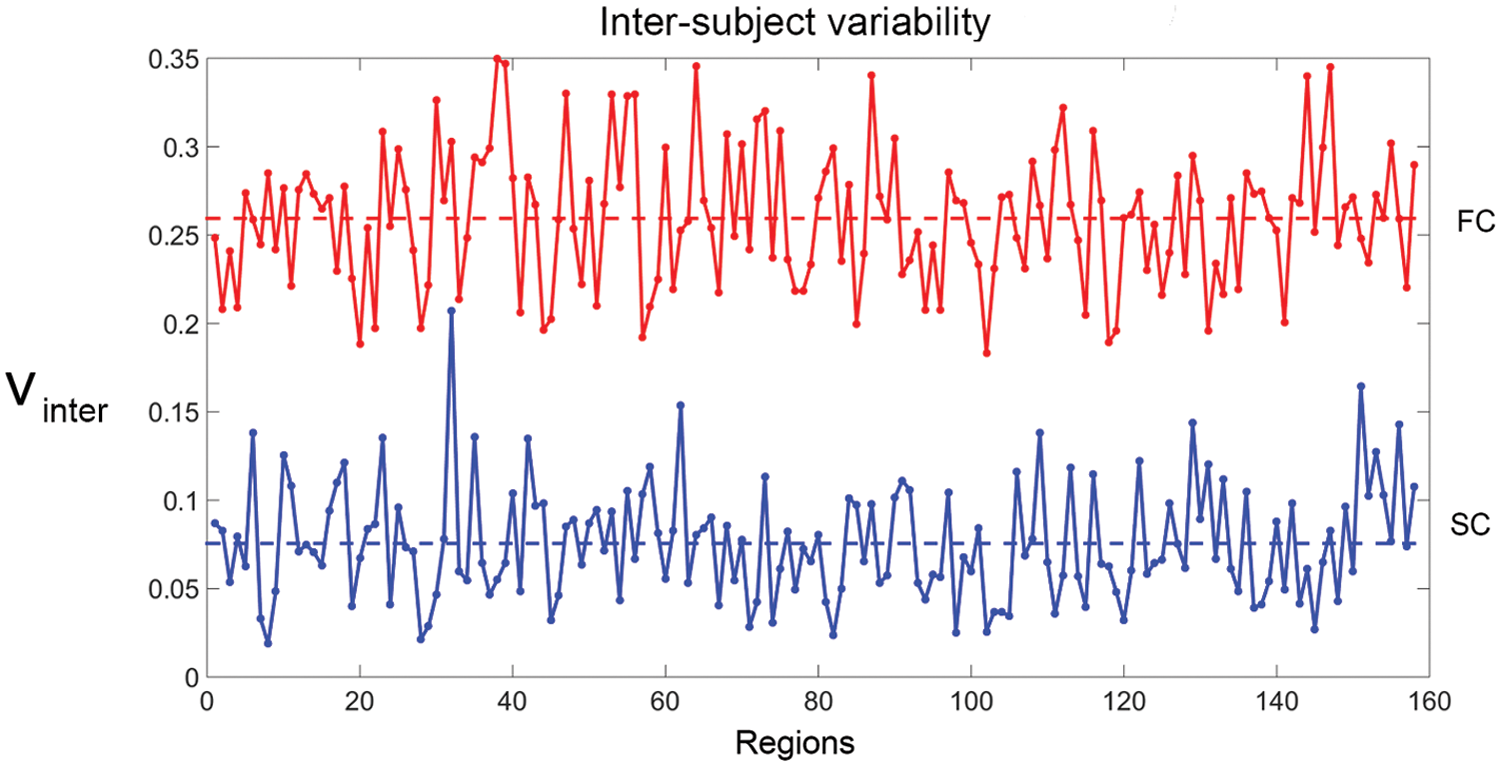
Inter-subject variability indices. Top: functional variability scores associated with each of the 159 regions (mean = 0.25, dotted line). Bottom: structural variability associated with each of the 159 regions (mean = 0.07, dotted line). Note that functional variability is globally higher than structural variability. Supplementary Data can be referred for label indexing. Color images available online at www.liebertpub.com/brain

Structural variability

To ensure the validity of the linear model used in this study (Fig. 2, step 4), the root mean square error (RMSE) was computed at all three time points. A value closer to 0 is preferred and indicates a good estimation of the structural residual maps. Figure 5 shows a validation of the structural residual maps ( \documentclass{aastex}\usepackage{amsbsy}\usepackage{amsfonts}\usepackage{amssymb}\usepackage{bm}\usepackage{mathrsfs}\usepackage{pifont}\usepackage{stmaryrd}\usepackage{textcomp}\usepackage{portland, xspace}\usepackage{amsmath, amsxtra}\usepackage{upgreek}\pagestyle{empty}\DeclareMathSizes{10}{9}{7}{6}\begin{document}$${ \bf V}_{inter}^t$$ \end{document} ) derived from linear least-squares regression. One can observe a linear relationship between intra-subject variability (V _intra) and the estimated group variability measures (1 − Sim ^t) in all cases, as well as near-zero RMSE values. Hence, the linear model employed in this study is conveniently applicable to SC analysis. In addition, the Pearson correlation (r _t) between group variability and intra-subject variability of the three dMRI sessions was: (r ₁ = 0.84, r ₂ = 0.79, r ₃ = 0.71, p < 0.001).

FIG. 5.

Linear relationship between group variability (1-Sim ^t) and intra-subject variability (V _intra) illustrated for the SC analysis (t = 3 sessions). The RMSE are also reported for all t = 3 regressions, indicating that the model employed in this study is relevant to SC analysis. RMSE, root mean squared error. Color images available online at www.liebertpub.com/brain

The resulting \documentclass{aastex}\usepackage{amsbsy}\usepackage{amsfonts}\usepackage{amssymb}\usepackage{bm}\usepackage{mathrsfs}\usepackage{pifont}\usepackage{stmaryrd}\usepackage{textcomp}\usepackage{portland, xspace}\usepackage{amsmath, amsxtra}\usepackage{upgreek}\pagestyle{empty}\DeclareMathSizes{10}{9}{7}{6}\begin{document}$${ \bf V}_{inter}^{SC}$$ \end{document} scores are illustrated in Figure 3 (right). Similar to that observed in the previous FC analysis, regions of low variability (purple–black) were also identified in the left and right motor network. On the other hand, higher variability was localized near language areas, as well as in the medial frontal lobe, and in the superior frontal gyrus.

Complementary to the previous results, Figure 4 (bottom) shows a quantitative indexing of structural variability indices ( \documentclass{aastex}\usepackage{amsbsy}\usepackage{amsfonts}\usepackage{amssymb}\usepackage{bm}\usepackage{mathrsfs}\usepackage{pifont}\usepackage{stmaryrd}\usepackage{textcomp}\usepackage{portland, xspace}\usepackage{amsmath, amsxtra}\usepackage{upgreek}\pagestyle{empty}\DeclareMathSizes{10}{9}{7}{6}\begin{document}$${ \bf V}_{inter}^{SC}$$ \end{document} ) for each of the 159 regions. The average structural variance was 0.07 ± 0.04 (0.12 ± 0.05 before correcting for intra-subject variability) and is considerably lower than the mean FC variability values (Fig. 4, dotted lines). Structural intra-subject variability values are reported in Supplementary Figure S2 (mean \documentclass{aastex}\usepackage{amsbsy}\usepackage{amsfonts}\usepackage{amssymb}\usepackage{bm}\usepackage{mathrsfs}\usepackage{pifont}\usepackage{stmaryrd}\usepackage{textcomp}\usepackage{portland, xspace}\usepackage{amsmath, amsxtra}\usepackage{upgreek}\pagestyle{empty}\DeclareMathSizes{10}{9}{7}{6}\begin{document}$${ \bf V}_{intra}^{SC}$$ \end{document} = 0.06 ± 0.03).

Structure–function relationship

To assess the potential link between functional and structural variability, variability indices between the two modalities were compared by using two separate approaches. First, region-to-region variations in \documentclass{aastex}\usepackage{amsbsy}\usepackage{amsfonts}\usepackage{amssymb}\usepackage{bm}\usepackage{mathrsfs}\usepackage{pifont}\usepackage{stmaryrd}\usepackage{textcomp}\usepackage{portland, xspace}\usepackage{amsmath, amsxtra}\usepackage{upgreek}\pagestyle{empty}\DeclareMathSizes{10}{9}{7}{6}\begin{document}$${ \bf V}_{inter}^{FC}$$ \end{document} were correlated with \documentclass{aastex}\usepackage{amsbsy}\usepackage{amsfonts}\usepackage{amssymb}\usepackage{bm}\usepackage{mathrsfs}\usepackage{pifont}\usepackage{stmaryrd}\usepackage{textcomp}\usepackage{portland, xspace}\usepackage{amsmath, amsxtra}\usepackage{upgreek}\pagestyle{empty}\DeclareMathSizes{10}{9}{7}{6}\begin{document}$${ \bf V}_{inter}^{SC}$$ \end{document} , yet they revealed a weak correlation (r = 0.15, p = 0.05). Second, we isolated regions exhibiting low (bottom 15%) FC and SC variability. The same was done for those with high variability (top 15%). Mutual regions of low and high variability are reported in Tables 1 and 2, along with their respective \documentclass{aastex}\usepackage{amsbsy}\usepackage{amsfonts}\usepackage{amssymb}\usepackage{bm}\usepackage{mathrsfs}\usepackage{pifont}\usepackage{stmaryrd}\usepackage{textcomp}\usepackage{portland, xspace}\usepackage{amsmath, amsxtra}\usepackage{upgreek}\pagestyle{empty}\DeclareMathSizes{10}{9}{7}{6}\begin{document}$${ \bf V}_{inter}^{FC}$$ \end{document} and \documentclass{aastex}\usepackage{amsbsy}\usepackage{amsfonts}\usepackage{amssymb}\usepackage{bm}\usepackage{mathrsfs}\usepackage{pifont}\usepackage{stmaryrd}\usepackage{textcomp}\usepackage{portland, xspace}\usepackage{amsmath, amsxtra}\usepackage{upgreek}\pagestyle{empty}\DeclareMathSizes{10}{9}{7}{6}\begin{document}$${ \bf V}_{inter}^{SC}$$ \end{document} variability indices.

Table 1.

Mutual Functional and Structural Regions of Low Variability (Bottom 15% of \documentclass{aastex}\usepackage{amsbsy}\usepackage{amsfonts}\usepackage{amssymb}\usepackage{bm}\usepackage{mathrsfs}\usepackage{pifont}\usepackage{stmaryrd}\usepackage{textcomp}\usepackage{portland, xspace}\usepackage{amsmath, amsxtra}\usepackage{upgreek}\pagestyle{empty}\DeclareMathSizes{10}{9}{7}{6}\begin{document}$${ \bf V}_{inter}^{FC}$$ \end{document} and \documentclass{aastex}\usepackage{amsbsy}\usepackage{amsfonts}\usepackage{amssymb}\usepackage{bm}\usepackage{mathrsfs}\usepackage{pifont}\usepackage{stmaryrd}\usepackage{textcomp}\usepackage{portland, xspace}\usepackage{amsmath, amsxtra}\usepackage{upgreek}\pagestyle{empty}\DeclareMathSizes{10}{9}{7}{6}\begin{document}$${ \bf V}_{inter}^{SC}$$ \end{document} )

Region	Brodmann area	Associated system	\documentclass{aastex}\usepackage{amsbsy}\usepackage{amsfonts}\usepackage{amssymb}\usepackage{bm}\usepackage{mathrsfs}\usepackage{pifont}\usepackage{stmaryrd}\usepackage{textcomp}\usepackage{portland, xspace}\usepackage{amsmath, amsxtra}\usepackage{upgreek}\pagestyle{empty}\DeclareMathSizes{10}{9}{7}{6}\begin{document}$${ \bf V}_{inter}^{FC}$$ \end{document}	\documentclass{aastex}\usepackage{amsbsy}\usepackage{amsfonts}\usepackage{amssymb}\usepackage{bm}\usepackage{mathrsfs}\usepackage{pifont}\usepackage{stmaryrd}\usepackage{textcomp}\usepackage{portland, xspace}\usepackage{amsmath, amsxtra}\usepackage{upgreek}\pagestyle{empty}\DeclareMathSizes{10}{9}{7}{6}\begin{document}$${ \bf V}_{inter}^{SC}$$ \end{document}
l-Central sulcus	BA1-4	Motor	0.20	0.03
l-Postcentral gyrus	BA1-4	Motor	0.20	0.02
r-Postcentral gyrus	BA1-4	Motor	0.18	0.03
l-Postcentral sulcus	BA1-4	Motor	0.22	0.04
r-Superior occipital gyrus	BA19	Visual	0.21	0.04
r-Sylvian fissure (posterior ceiling)	BA41–43	Motor	0.21	0.04

Table 2.

Mutual Functional and Structural Regions of High Variability (Top 15% of \documentclass{aastex}\usepackage{amsbsy}\usepackage{amsfonts}\usepackage{amssymb}\usepackage{bm}\usepackage{mathrsfs}\usepackage{pifont}\usepackage{stmaryrd}\usepackage{textcomp}\usepackage{portland, xspace}\usepackage{amsmath, amsxtra}\usepackage{upgreek}\pagestyle{empty}\DeclareMathSizes{10}{9}{7}{6}\begin{document}$${ \bf V}_{inter}^{FC}$$ \end{document} and \documentclass{aastex}\usepackage{amsbsy}\usepackage{amsfonts}\usepackage{amssymb}\usepackage{bm}\usepackage{mathrsfs}\usepackage{pifont}\usepackage{stmaryrd}\usepackage{textcomp}\usepackage{portland, xspace}\usepackage{amsmath, amsxtra}\usepackage{upgreek}\pagestyle{empty}\DeclareMathSizes{10}{9}{7}{6}\begin{document}$${ \bf V}_{inter}^{SC}$$ \end{document} )

Region	Brodmann area	Associated system	\documentclass{aastex}\usepackage{amsbsy}\usepackage{amsfonts}\usepackage{amssymb}\usepackage{bm}\usepackage{mathrsfs}\usepackage{pifont}\usepackage{stmaryrd}\usepackage{textcomp}\usepackage{portland, xspace}\usepackage{amsmath, amsxtra}\usepackage{upgreek}\pagestyle{empty}\DeclareMathSizes{10}{9}{7}{6}\begin{document}$${ \bf V}_{inter}^{FC}$$ \end{document}	\documentclass{aastex}\usepackage{amsbsy}\usepackage{amsfonts}\usepackage{amssymb}\usepackage{bm}\usepackage{mathrsfs}\usepackage{pifont}\usepackage{stmaryrd}\usepackage{textcomp}\usepackage{portland, xspace}\usepackage{amsmath, amsxtra}\usepackage{upgreek}\pagestyle{empty}\DeclareMathSizes{10}{9}{7}{6}\begin{document}$${ \bf V}_{inter}^{SC}$$ \end{document}
l-Parahippocampal gyrus	BA34	Limbic	0.31	0.14
l-Subcallosal gyrus/BA25	BA25	Limbic	0.30	0.21
l-Sulcus intermedius primus (of Jensen)	BA39, 40	Language	0.33	0.11
r-Sulcus intermedius primus (of Jensen)	BA39, 40	Language	0.30	0.14
r-Superior temporal gyrus (planum temporale)	BA22	Language/Auditory	0.30	0.14
l-Superior temporal sulcus	BA21	Language/Auditory	0.32	0.11

Low inter-subject variability

To qualitatively illustrate SC in a region of low variability, Figure 6 presents a group mosaic of the left central sulcus tractography (anterior view). In this example, streamlines show high consistency with multiple inter-hemispheric connections sites across different subjects (e.g., CC, yellow arrowheads). The CST and its projection fibers is also represented across all subjects. Red arrowheads indicate intra-hemispheric similarities. Streamlines were visualized by using Orientation-Dependent Transparency Rendering (Tax et al., 2015) to improve the rendering of hidden structures (e.g., central sulcus region, green isosurface).

FIG. 6.

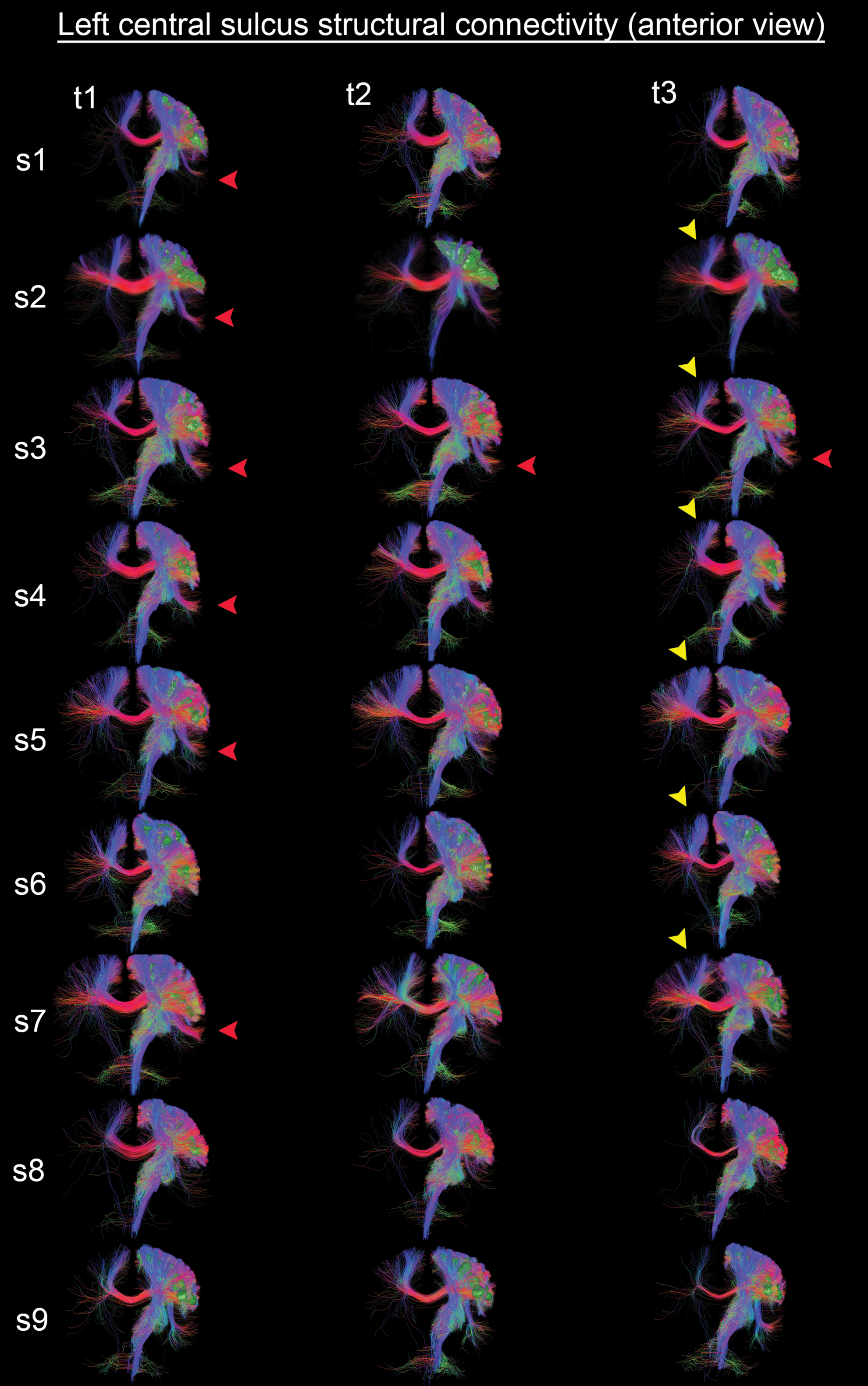
Left central sulcus tractography (anterior view) shows high consistency with multiple commissural connections sites (e.g., corpus callosum, yellow arrowheads). Red arrowheads indicate intra-hemispheric similarities. Streamlines were downsampled by a factor 10 for visualization. Visualization was done by using Orientation-Dependent Transparency Rendering (Tax et al., 2015). Color images available online at www.liebertpub.com/brain

High inter-subject variability

In contrast, Figure 7 shows tractography in a region of higher variability (i.e., left parahippocampal gyrus, lateral view). In this case, streamlines show a larger variability with multiple intra-hemispheric connections sites (e.g., cingulum). One can also notice differences in the orbitofrontal projection of the uncinate fasciculus for multiple subjects. Intra-subject differences are indicated with yellow arrowheads, and inter-subject differences are pointed out with paired red arrowheads. Streamlines were also rendered transparent for a better appreciation of the parahippocampal gyrus isosurface (orange).

FIG. 7.

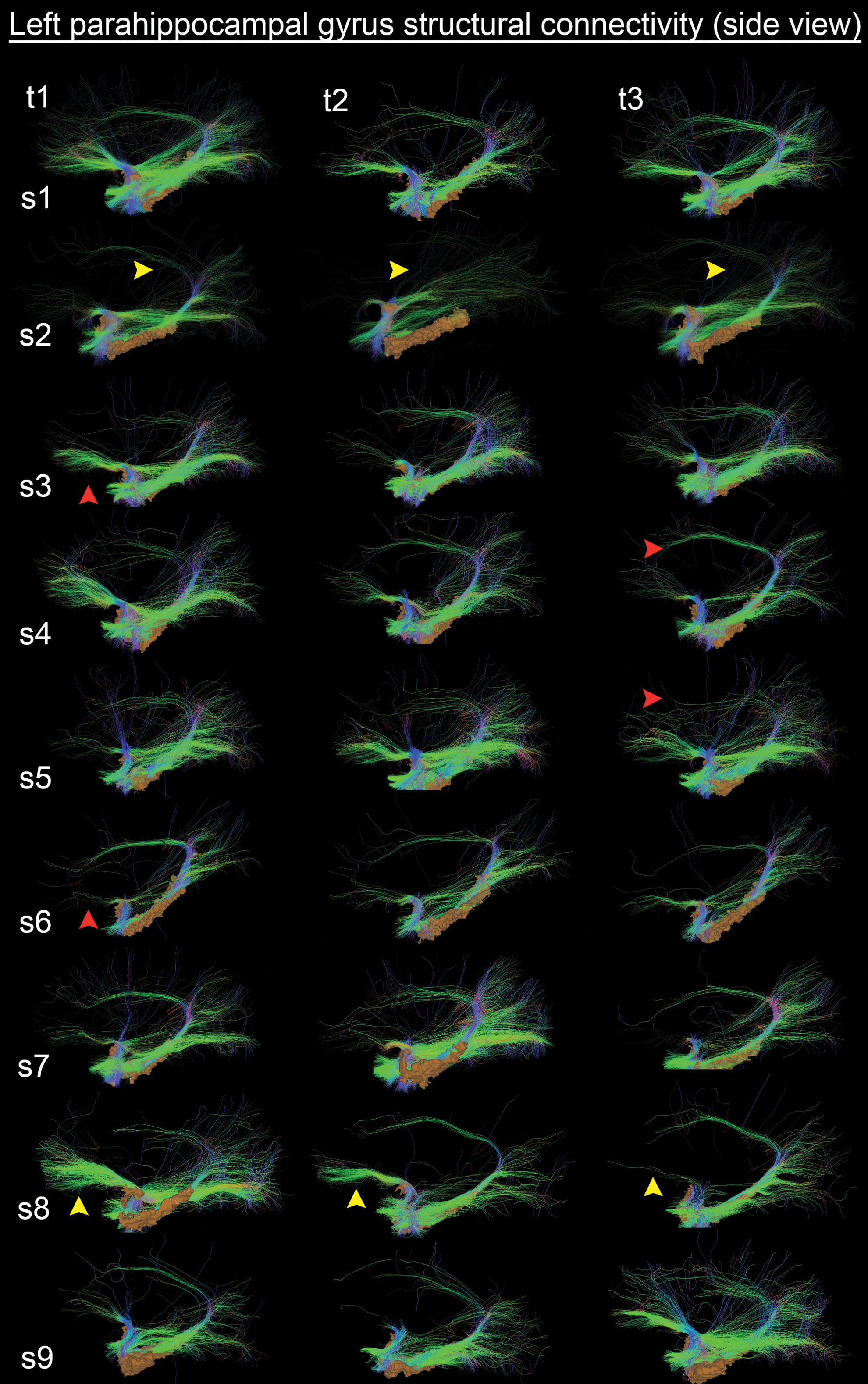
Left parahippocampal gyrus tractography (lateral view) shows a large variability with multiple association connections sites (e.g., cingulum and uncinate fasciculus). Yellow arrowheads indicate intra-subject differences, and red arrowheads indicate inter-subject differences. Streamlines were downsampled by a factor 10 for visualization. Visualization was done by using Orientation-Dependent Transparency Rendering (Tax et al., 2015). Color images available online at www.liebertpub.com/brain

Confounding factors correction

We further explored the effect of region size on structural variability. Figure 8 shows the effect of seeding surface area (left) and number of streamlines (right, normalized) on inter-subject variability scores for all subjects. The results indicated no correlation between \documentclass{aastex}\usepackage{amsbsy}\usepackage{amsfonts}\usepackage{amssymb}\usepackage{bm}\usepackage{mathrsfs}\usepackage{pifont}\usepackage{stmaryrd}\usepackage{textcomp}\usepackage{portland, xspace}\usepackage{amsmath, amsxtra}\usepackage{upgreek}\pagestyle{empty}\DeclareMathSizes{10}{9}{7}{6}\begin{document}$${ \bf V}_{inter}^{SC}$$ \end{document} and seeding surface area (r = −0.03, p = 0.73), nor with the number of streamlines of each region (r = −0.02, p = 0.75). Specifically, areas of high inter-subject variability were not associated with those of a low surface area and vice versa. Note that the number of streamlines connecting each region was defined as the sum of each element of M for a given row, and before row normalization of M. Variability indices without correction for structural confounds are illustrated in Supplementary Figure S3.

FIG. 8.

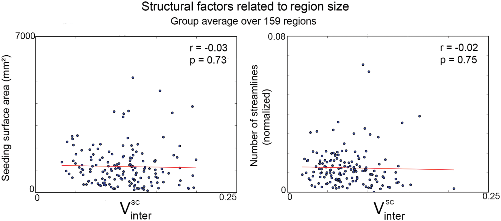
Structural factors related to region size averaged across subjects. Left: Seeding surface area of each region shows no correlation with inter-subject variability (r = −0.03, p = 0.73). Right: Number of streamlines within each region also revealed no link with inter-subject variability (r = −0.02, p = 0.75). Color images available online at www.liebertpub.com/brain

Discussion

A major hurdle in comparing FC with SC is that it is nearly impossible to accurately quantify their respective strengths. To resolve this, we adopted a recently described repeated-measures approach for FC and applied it to tractography-based SC. Rather than correlating the “strength” of FC to that of SC, we computed inter-individual variability in FC of major cortical and sub-cortical areas and compared it with corresponding inter-individual variability in SC. Some areas exhibited mutually low (e.g., primary motor cortex) and high (e.g., language area) \documentclass{aastex}\usepackage{amsbsy}\usepackage{amsfonts}\usepackage{amssymb}\usepackage{bm}\usepackage{mathrsfs}\usepackage{pifont}\usepackage{stmaryrd}\usepackage{textcomp}\usepackage{portland, xspace}\usepackage{amsmath, amsxtra}\usepackage{upgreek}\pagestyle{empty}\DeclareMathSizes{10}{9}{7}{6}\begin{document}$${ \bf V}_{inter}^{FC}$$ \end{document} and \documentclass{aastex}\usepackage{amsbsy}\usepackage{amsfonts}\usepackage{amssymb}\usepackage{bm}\usepackage{mathrsfs}\usepackage{pifont}\usepackage{stmaryrd}\usepackage{textcomp}\usepackage{portland, xspace}\usepackage{amsmath, amsxtra}\usepackage{upgreek}\pagestyle{empty}\DeclareMathSizes{10}{9}{7}{6}\begin{document}$${ \bf V}_{inter}^{SC}$$ \end{document} , though across the whole brain, the correlation between the two was very weak. These results highlight the continuing challenge in interpreting inter-individual differences in FC.

Low inter-subject variability

Inter-subject variability mapping revealed key regions of the brain with low structural and functional variability (Figs. 3 and 4). Specifically, the left and right post-central gyri, left central and post-central sulci were the most reproducible in terms of connectivity overall (all below 0.04 for the SC analysis, and all below 0.22 for the FC analysis). This result indicates that, at least in these sensorimotor regions, inference of brain connectivity using tractography and resting-state functional magnetic resonance imaging (rs-fMRI) is increasingly reliable compared with everywhere else in the brain. These results are also in line with those of Mueller and associates (2013), Gonzalez-Castillo and colleagues (2014), Chen and associates (2015), and Finn and colleagues (2015), who reported that connectivity patterns of motor regions were more consistent than the ones associated to higher order cognitive processes (e.g., memory and language).

When qualitatively looking at the underlying WM motor connections (Fig. 6), tractography of the left sulcus central showed considerable reproducibility in terms of connectivity patterns (e.g., commissural CC connections and cortical fanning of the CST). This low variability is closely in line with previous studies that compared functional variability with evolutionary cortex expansion (Mueller et al., 2013), which also reveals lower surface expansion indices within the motor network. Another group also reported low structural variability in brain gyrification of the motor cortex, which may explain its consistent connectivity profile (Hill et al., 2010).

Indeed, with streamline tractography seeded from the GM/WM interface, the first few voxels in streamline propagation are crucial to determine the final shape and course of the bundle. Likewise, other studies recently demonstrated that long-range connections are impeded by the superficial layers of GM (Burgel et al., 2006; Reveley et al., 2015). This degree of gyrification and layering of the GM may explain why some of the WM fascicles are consistently reproduced across subjects with tractography. Our findings also revealed lower variability within the posterior end of the Sylvian fissure, on the right side of the brain. This lower variability may be due to the fact that this sulcus is one of the earliest developing sulci in the human brain (Chi et al., 1977). Interestingly, the human secondary somatosensory cortex is also located at the ceiling of the Sylvian fissure (Penfield and Jasper, 1954), in line with our aforementioned motor cortex findings.

Low variance was also identified in the right superior occipital gyrus, where multiple WM pathways connect. Visual inspection of this area revealed the following underlying major WM bundles: the inferior longitudinal fasciculus, optic tracts, and splenium of the CC. For consideration, changes of cortical thickness and corresponding WM microstructure during brain development can also play an important role in defining individual brain regions, as these regions evolve at a different rate (Jeon et al., 2015). For example, the optic radiation (OR) is a well-understood fascicle with the primary function of transmitting visual information to the visual cortex. It is also among the few primary WM fiber pathways to attain complete myelination in the early developmental stages (Kinney et al., 1988). It is generally believed that the OR projects to the calcarine fissure (in the primary visual cortex, V1), though it has been shown recently that it may reach V2 and V3 as well (Alvarez et al., 2015; Renauld et al., 2016; Chamberland et al., 2017). This may indicate that after a certain age, this fascicle is already fully developed and its connectivity profile is less likely to vary across healthy subjects. In this study, potential confounding factors related to age difference (Mattay et al., 2002; Nenonen et al., 2015) were reduced by the inclusion of a homogeneous subject sample (i.e., nine young adults, mean age 25 years ±3.1; range 21–30).

High inter-subject variability

Conversely, higher variability profiles are noticeable on the medial aspect of the temporal lobe. Specifically, the parahippocampal gyrus and the subcallosal gyrus (BA25) (two regions that are part of the limbic system) were among the highest varying regions of this study, both functionally and structurally. The parahippocampal gyrus plays an important role in memory retrieval (Whittingstall et al., 2014) and is composed of multiple interdigitating association fascicles (Schmahmann and Pandya, 2006; Yogarajah et al., 2008) such as the uncinate fasciculus, the temporal projections of the cingulum and of the fornix, the medial and inferior longitudinal fasciculi, and the inferior fronto-occipital fasciculus (Catani et al., 2003; Catani and Thiebaut De Schotten, 2012). This highly complex configuration can potentially lead to a widespread connectivity spectrum, as denoted by our variability mapping results. For instance, the orbitofrontal projections of the uncinate fasciculus were either absent from this region or partially represented across multiple subjects.

Interestingly, variability indices were also the largest in the temporo-parietal cortex for both FC and SC analysis. Notably, the sulcus intermedius primus of Jensen (bilateral) revealed signs of higher inter-subject variability for both structural (left: 0.11, right: 0.14) and functional (left: 0.33, right: 0.30) analysis. This region marks the boundary between the supramarginal and angular gyri (Kiriyama et al., 2009) and closely overlaps with Wernicke's area. In addition, the right superior temporal gyrus (planum temporale) is a cortical region of the temporal lobe also overlapping Wernicke's area. Studies also revealed a preferential leftward development of this cortical area (Geschwind and Levitsky, 1968; Steinmetz, 1996). Even though this area is most often found on the left side of the brain, a lack of functional specificity on the contra-lateral hemisphere may also lead to a higher inter-subject variability, indicating potential variable WM connectivity. Our results also indicated higher variability within the left superior temporal sulcus. This unilateral profile is closely related with the brain lateralization of higher cognitive functions such as language [e.g., Broca's area Catani and Mesulam (2008); Lurito and Dzemidzic (2001); Vassal et al. (2016)]. Other structure–function relationships studies have previously reported a lateralization of FA values and number of streamlines within the arcuate fasciculus (underlying WM pathway involved with language) (Powell et al., 2006; Vernooij et al., 2007). Such structural asymmetries may also be related to a highly specific functional lateralization. The group of Vassal and colleagues (2016) also reported leftward lateralization of the arcuate fasciculus using diffusion tensor imaging, and major inter-hemispheric differences in streamlines connecting Broca's area and Wernicke's area were noticed in more than half of their subjects.

SC confounding factors

Our choice of local modeling of the diffusion data worked toward reducing potential connectivity bias by being robust to crossing and kissing regions. Indeed, it is generally accepted by the community that HARDI-based techniques can overcome the limitations of diffusion tensor imaging (DTI) tractography by resolving the many crossing fiber regions in the brain (Descoteaux, 2015; Farquharson et al., 2013; Neher et al., 2015; Nimsky et al., 2016; Seunarine and Alexander, 2009; Tournier et al., 2011). Possible structural confounding factors of this study can be related to the construction of SC matrices (Jones et al., 2013; Smith et al., 2015). For instance, a region expressing a higher volume (mm³) may also show higher reproducibility due to an over-representation in the number of underlying streamlines. Here, potential bias toward seed density was mitigated by initiating tractography from the WM/GM interface (Girard et al., 2014) instead of using the whole WM volume. In addition, SC matrices were also normalized across regions and subjects to account for various streamline counts and inter-subject variability values were also corrected for seeding surface area (mm²) to remove any remaining bias toward brain region size. This step was performed independently of the variability pipeline to ensure matching processing between rs-fMRI and dMRI connectivity matrices. As a result, no significant correlation between inter-subject variability indices and region surface area (r = −0.03, p = 0.73) was observed. Further, the number of streamlines in each region showed no significant correlation with variance measures (r = −0.02, p = 0.75, Supplementary Fig. S3). For these reasons, the heterogeneous size of the parcellated brain regions cannot explain our \documentclass{aastex}\usepackage{amsbsy}\usepackage{amsfonts}\usepackage{amssymb}\usepackage{bm}\usepackage{mathrsfs}\usepackage{pifont}\usepackage{stmaryrd}\usepackage{textcomp}\usepackage{portland, xspace}\usepackage{amsmath, amsxtra}\usepackage{upgreek}\pagestyle{empty}\DeclareMathSizes{10}{9}{7}{6}\begin{document}$${ \bf V}_{inter}^{SC}$$ \end{document} results. In terms of \documentclass{aastex}\usepackage{amsbsy}\usepackage{amsfonts}\usepackage{amssymb}\usepackage{bm}\usepackage{mathrsfs}\usepackage{pifont}\usepackage{stmaryrd}\usepackage{textcomp}\usepackage{portland, xspace}\usepackage{amsmath, amsxtra}\usepackage{upgreek}\pagestyle{empty}\DeclareMathSizes{10}{9}{7}{6}\begin{document}$${ \bf V}_{inter}^{FC}$$ \end{document} , our brain parcellation strategy (Freesurfer) yielded results very similar to the vertex approach used by Mueller and colleagues (2013), indicating that our methodological approach (large parcellated brain areas, less number of subjects and scans) also did not bias the results. The use of 10 seeds per voxel (1 mm isotropic grid, e.g., >2M seeds) also aimed at avoiding potential seed bias and ensured a stabilized edge metric (i.e., weights of M represented by the normalized streamline count) (Colon-Perez et al., 2015; Girard et al., 2014). In a pioneer study by the group of Hagmann and associates (2007), the authors reported that one-third to half of streamlines did not reach the WM/GM interface mask and, thus, were excluded from the SC analysis. The tractography algorithm employed in this study ensured that streamlines did not prematurely terminate in the WM. The inclusion of subscortical regions (e.g., thalamus) also enabled a better representation of important pathways such as the optic radiations in the derived connectivity matrices.

Weak link between functional and structural inter-subject variability

As described earlier, certain brain regions showing the lowest \documentclass{aastex}\usepackage{amsbsy}\usepackage{amsfonts}\usepackage{amssymb}\usepackage{bm}\usepackage{mathrsfs}\usepackage{pifont}\usepackage{stmaryrd}\usepackage{textcomp}\usepackage{portland, xspace}\usepackage{amsmath, amsxtra}\usepackage{upgreek}\pagestyle{empty}\DeclareMathSizes{10}{9}{7}{6}\begin{document}$${ \bf V}_{inter}^{FC}$$ \end{document} also exhibited low \documentclass{aastex}\usepackage{amsbsy}\usepackage{amsfonts}\usepackage{amssymb}\usepackage{bm}\usepackage{mathrsfs}\usepackage{pifont}\usepackage{stmaryrd}\usepackage{textcomp}\usepackage{portland, xspace}\usepackage{amsmath, amsxtra}\usepackage{upgreek}\pagestyle{empty}\DeclareMathSizes{10}{9}{7}{6}\begin{document}$${ \bf V}_{inter}^{SC}$$ \end{document} , as did areas with the highest \documentclass{aastex}\usepackage{amsbsy}\usepackage{amsfonts}\usepackage{amssymb}\usepackage{bm}\usepackage{mathrsfs}\usepackage{pifont}\usepackage{stmaryrd}\usepackage{textcomp}\usepackage{portland, xspace}\usepackage{amsmath, amsxtra}\usepackage{upgreek}\pagestyle{empty}\DeclareMathSizes{10}{9}{7}{6}\begin{document}$${ \bf V}_{inter}^{FC}$$ \end{document} . However, across all regions, \documentclass{aastex}\usepackage{amsbsy}\usepackage{amsfonts}\usepackage{amssymb}\usepackage{bm}\usepackage{mathrsfs}\usepackage{pifont}\usepackage{stmaryrd}\usepackage{textcomp}\usepackage{portland, xspace}\usepackage{amsmath, amsxtra}\usepackage{upgreek}\pagestyle{empty}\DeclareMathSizes{10}{9}{7}{6}\begin{document}$${ \bf V}_{inter}^{SC}$$ \end{document} was significantly lower than \documentclass{aastex}\usepackage{amsbsy}\usepackage{amsfonts}\usepackage{amssymb}\usepackage{bm}\usepackage{mathrsfs}\usepackage{pifont}\usepackage{stmaryrd}\usepackage{textcomp}\usepackage{portland, xspace}\usepackage{amsmath, amsxtra}\usepackage{upgreek}\pagestyle{empty}\DeclareMathSizes{10}{9}{7}{6}\begin{document}$${ \bf V}_{inter}^{FC}$$ \end{document} (0.07 ± 0.04 vs. 0.25 ± 0.04, respectively) and they were poorly correlated (r = 0.15, p = 0.05). It is possible that functional variability is greater on average than structural variability because functional variability can be sensitive to previous life experience and genetic factors (Vaidya and Gordon, 2013) and can vary dynamically (Hutchison et al., 2013). Indeed, FC is known to reflect a combination of dynamic signals that varies across the brain of each individual (Smith et al., 2013). For example, in the motor cortex, both variability measures were relatively low, though \documentclass{aastex}\usepackage{amsbsy}\usepackage{amsfonts}\usepackage{amssymb}\usepackage{bm}\usepackage{mathrsfs}\usepackage{pifont}\usepackage{stmaryrd}\usepackage{textcomp}\usepackage{portland, xspace}\usepackage{amsmath, amsxtra}\usepackage{upgreek}\pagestyle{empty}\DeclareMathSizes{10}{9}{7}{6}\begin{document}$${ \bf V}_{inter}^{FC}$$ \end{document} was almost five times higher than \documentclass{aastex}\usepackage{amsbsy}\usepackage{amsfonts}\usepackage{amssymb}\usepackage{bm}\usepackage{mathrsfs}\usepackage{pifont}\usepackage{stmaryrd}\usepackage{textcomp}\usepackage{portland, xspace}\usepackage{amsmath, amsxtra}\usepackage{upgreek}\pagestyle{empty}\DeclareMathSizes{10}{9}{7}{6}\begin{document}$${ \bf V}_{inter}^{SC}$$ \end{document} , indicating that the SC profile of the motor cortex is far more similar across healthy subjects than that of its FC profile. The exact reasons behind this mismatch are unclear.

One possible explanation for this result is that the bulk of the reconstructed streamlines emanating from the motor cortex are made up of either the CC or the CST, with little to no terminations observed in other cortical areas. FC, on the other hand, may be visible in these areas due to indirect anatomical connections, thus explaining its higher inter-individual variability as shown in Supplementary Figure S4. Even though FC of the left central sulcus showed similar patterns between different subjects, individual differences are identifiable in the cerebellum and are supported by direct anatomical pathways. However, SC revealed no direct link between parahippocampal connectivity and the left central sulcus. Indirect structural pathways may, therefore, play a key role in explaining the mismatch between \documentclass{aastex}\usepackage{amsbsy}\usepackage{amsfonts}\usepackage{amssymb}\usepackage{bm}\usepackage{mathrsfs}\usepackage{pifont}\usepackage{stmaryrd}\usepackage{textcomp}\usepackage{portland, xspace}\usepackage{amsmath, amsxtra}\usepackage{upgreek}\pagestyle{empty}\DeclareMathSizes{10}{9}{7}{6}\begin{document}$${ \bf V}_{inter}^{FC}$$ \end{document} and \documentclass{aastex}\usepackage{amsbsy}\usepackage{amsfonts}\usepackage{amssymb}\usepackage{bm}\usepackage{mathrsfs}\usepackage{pifont}\usepackage{stmaryrd}\usepackage{textcomp}\usepackage{portland, xspace}\usepackage{amsmath, amsxtra}\usepackage{upgreek}\pagestyle{empty}\DeclareMathSizes{10}{9}{7}{6}\begin{document}$${ \bf V}_{inter}^{SC}$$ \end{document} , which remains an active area of research nowadays (Jbabdi et al., 2015).

Another possible explanation is that diffusion- and BOLD-based measures of brain structure and function, respectively, are sensitive to different sources of noise. For instance, BOLD signal correlations in areas that are highly vascularized may be artificially inflated compared with other regions (Curtis et al., 2014; Kazan et al., 2016; Vigneau-Roy et al., 2014). On the other hand, blood vessels may interfere with diffusion measures, potentially leading to an incorrect estimation of SC due to intravoxel incoherent motion (Le Bihan, 2008). Taken together, the sum of all those sources of variability effectively contributes toward establishing inter-subject variability.

Clinical implications

Fingerprint patterns of FC can be used to identify subjects across sessions and individuals (Finn et al., 2015), indicating that the topology of the brain substantially differs between individuals. Assuming that patterns of spatial heterogeneity are also present in SC, our finding is also of clinical importance with the recent advances in surgical approaches based on connectomics (Griffa et al., 2013; Meola et al., 2016; Yu et al., 2016). For instance, a region of inter-individual variability can have potential influence on preoperative planning as the spatial localization of this area may vary from one subject to another. As of today, rs-fMRI imaging protocols are often used in clinical studies to guide surgical gesture. In addition, tractography has been shown to be valuable for surgical planning, and neurosurgeons and radiologists are mostly convinced of the importance of achieving an accurate delineation of WM pathways using tractography (Duffau, 2005; Leclercq et al., 2010; Nimsky et al., 2016). Defining accurate boundaries is critical in surgery targeting frontal and temporal regions (e.g., space-occupying lesion, temporal lobe epilepsy), as these areas exhibit higher variability between subjects. With the advent of personalized medicine (Wang et al., 2015), we believe that such a tailored mapping may improve decision making and is likely to impact pre-operative planning approaches, where capturing the idiosyncrasies of individuals is paramount.

Conclusion

In this study, we generated brain functional and structural inter-subject variability maps by taking into account the intra-subject variability using a test–retest approach. With this approach, we showed that structural inter-subject variability was globally lower than functional variability. Our approach also revealed that variability indices were smallest in motor areas for both functional and structural analysis, indicating proper reproducibility within this region. Our results also indicate that functional and structural variability profiles were less consistent near the memory and language areas of the brain. These findings suggest that, at least in these regions, functional inter-subject variability can be explained by the structural organization of the brain. In other words, stable FC does not always imply stable SC for the rest of the brain. Altogether, this study highlights a different aspect of brain connectivity analysis, by not only exploring the link between FC and SC but also investigating the variability between them.

Footnotes

Acknowledgments

The authors would like to acknowledge the funding agencies that have supported this research: Natural Sciences and Engineering Research Council of Canada (NSERC) Discovery Grants, QBIN (Quebec Bio-Imaging Network), and the FMSS graduate scholarship program. Main author M.C. was supported by the Alexander Graham Bell Canada Graduate Scholarships-Doctoral Program (CGS-D3) from the NSERC at the time.

Author Disclosure Statement

No competing financial interests exist.

References

Alvarez

, Schwarzkopf

, Clark

. 2015. Extrastriate projections in human optic radiation revealed by fMRI-informed tractography. Brain Struct Funct, 220:2519–2532.

Bandettini

, Jesmanowicz

, Wong

, Hyde

. 1993. Processing strategies for time-course data sets in functional MRI of the human brain. Magn Reson Med, 30:161–173.

Bastiani

, Shah

, Goebel

, Roebroeck

. 2012. Human cortical connectome reconstruction from diffusion weighted MRI: the effect of tractography algorithm. Neuroimage, 62:1732–1749.

Bernier

, Chamberland

, Houde

, Descoteaux

, Whittingstall

. 2014. Using fMRI non local means denoising to uncover activation in sub-cortical structures at 1.5 T for guided HARDI tractography. Front Hum Neurosci, 8:715.

Biswal

, Yetkin

, Haughton

, Hyde

. 1995. Functional connectivity in the motor cortex of resting human brain using echo-planar MRI. Magn Reson Med, 34:537–541.

Bowman

, Zhang

, Derado

, Chen

. 2012. Determining functional connectivity using fMRI data with diffusion-based anatomical weighting. Neuroimage, 62:1769–1779.

Buckner

, Krienen

, Yeo

. 2013. Opportunities and limitations of intrinsic functional connectivity MRI. Nat Neurosci, 16:832–837.

Burgel

, Amunts

, Hoemke

, Mohlberg

, Gilsbach

, Zilles

. 2006. White matter fiber tracts of the human brain: three-dimensional mapping at microscopic resolution, topography and inter-subject variability. Neuroimage, 29:1092–1105.

Cammoun

, Gigandet

, Meskaldji

, Thiran

, Sporns

, Do

, et al. 2012. Mapping the human connectome at multiple scales with diffusion spectrum MRI. J Neurosci Methods, 203:386–397.

10.

Catani

, Jones

, Donato

, Ffytche

. 2003. Occipito-temporal connections in the human brain. Brain, 126:2093–2107.

11.

Catani

, Mesulam

. 2008. The arcuate fasciculus and the disconnection theme in language and aphasia: history and current state. Cortex, 44:953–961.

12.

Catani

, Thiebaut De Schotten

. 2012. Atlas of Human Brain Connections. New York, NY: Oxford University Press. Includes bibliographical references and index.

13.

Chamberland

, Bernier

, Fortin

, Whittingstall

, Descoteaux

. 2015. 3D interactive tractography-informed resting-state fMRI connectivity. Front Neurosci, 9:275.

14.

Chamberland

, Scherrer

, Prabhu

, Madsen

, Fortin

, Whittingstall

, et al. 2017. Active delineation of Meyer's loop using oriented priors through MAGNEtic tractography (MAGNET). Hum Brain Mapp, 38:509–527.

15.

Chen

, Xu

, Zhou

, Wang

, Yang

, Wang

, et al. 2015. Individual variability and test–retest reliability revealed by ten repeated resting-state brain scans over one month. PLoS One, 10:e0144963.

16.

Cheng

, Wang

, Sheng

, Kronenberger

, Mathews

, Hummer

, Saykin

. 2012. Characteristics and variability of structural networks derived from diffusion tensor imaging. Neuroimage, 61:1153–1164.

17.

Chi

, Dooling

, Gilles

. 1977. Gyral development of the human brain. Ann Neurol, 1:86–93.

18.

Colon-Perez

, Spindler

, Goicochea

, Triplett

, Parekh

, Montie

, et al. 2015. Dimensionless, scale invariant, edgeweight metric for the study of complex structural networks. PLoS One, 10:e0131493.

19.

Coupe

, Yger

, Prima

, Hellier

, Kervrann

, Barillot

. 2008. An optimized blockwise nonlocal means denoising filter for 3-D magnetic resonance images. IEEE Trans Med Imaging, 27:425–441.

20.

Cox

. 1996. AFNI: software for analysis and visualization of functional magnetic resonance neuroimages. Comput Biomed Res, 29:162–173.

21.

Curtis

, Hutchison

, Menon

. 2014. Phase based venous suppression in resting-state BOLD GE-FMRI. Neuroimage, 100:51–59.

22.

Damoiseaux

, Rombouts

SARB

, Barkhof

, Scheltens

, Stam

, Smith

, Beckmann

. 2006. Consistent resting-state networks across healthy subjects. Proc Natl Acad Sci U S A, 103:13848–13853.

23.

Descoteaux

. 2015. High angular resolution diffusion imaging (HARDI). Wiley Encyclopedia of Electrical and Electronics Engineering. John Wiley & Sons, Inc., p. 1.

24.

Destrieux

, Fischl

, Dale

, Halgren

. 2010. Automatic parcellation of human cortical gyri and sulci using standard anatomical nomenclature. Neuroimage, 53:1–15.

25.

Duffau

. 2005. Lessons from brain mapping in surgery for low-grade glioma: insights into associations between tumour and brain plasticity. Lancet Neurol, 4:476–486.

26.

Farquharson

, Tournier

, Calamante

, Fabinyi

, Schneider-Kolsky

, Jackson

, Connelly

. 2013. White matter fiber tractography: why we need to move beyond DTI. J Neurosurg, 118:1367–1377.

27.

Finn

, Shen

, Scheinost

, Rosenberg

, Huang

, Chun

, et al. 2015. Functional connectome fingerprinting: identifying individuals using patterns of brain connectivity. Nat Neurosci, 18:1664–1671.

28.

Fischl

, van der Kouwe

, Destrieux

, Halgren

, Segonne

, Salat

, et al. 2004. Automatically parcellating the human cerebral cortex. Cereb Cortex, 14:11–22.

29.

Fornito

, Zalesky

, Breakspear

. 2015. The connectomics of brain disorders. Nat Rev Neurosci, 16:159–172.

30.

Garyfallidis

, Brett

, Amirbekian

, Rokem

, van der Walt

, Descoteaux

, Nimmo-Smith

. 2014. Dipy, a library for the analysis of diffusion MRI data. Front Neuroinform, 8:8.

31.

Gaser

, Schlaug

. 2003. Brain structures differ between musicians and non-musicians. J Neurosci, 23:9240–9245.

32.

Geschwind

, Levitsky

. 1968. Human brain: left-right asymmetries in temporal speech region. Science, 161:186–187.

33.

Ghaziri

, Tucholka

, Girard

, Houde

, Boucher

, Gilbert

, et al. 2017. The corticocortical structural connectivity of the human insula. Cereb Cortex, 27:1216–1228.

34.

Ghumman

, Fortin

, Noel-Lamy

, Cunnane

, Whittingstall

. 2016. Exploratory study of the effect of brain tumors on the default mode network. J Neurooncol, 128:437–444.

35.

Girard

, Whittingstall

, Deriche

, Descoteaux

. 2014. Towards quantitative connectivity analysis: reducing tractography biases. Neuroimage, 98:266–278.

36.

Girard

, Whittingstall

, Deriche

, Descoteaux

. Studying White Matter Tractography Reproducibility Through Connectivity Matrices. In International Symposium on Magnetic Resonance in Medicine, Toronto, Canada, 2015.

37.

Gong

, He

, Concha

, Lebel

, Gross

, Evans

, Beaulieu

. 2009. Mapping anatomical connectivity patterns of human cerebral cortex using in vivo diffusion tensor imaging tractography. Cereb Cortex, 19:524–536.

38.

Goni

, van den Heuvel

, Avena-Koenigsberger

, Velez de Mendizabal

, Betzel

, Griffa

, et al. 2014. Resting-brain functional connectivity predicted by analytic measures of network communication. Proc Natl Acad Sci U S A, 111:833–838.

39.

Gonzalez-Castillo

, Handwerker

, Robinson

, Hoy

, Buchanan

, Saad

, Bandettini

. 2014. The spatial structure of resting state connectivity stability on the scale of minutes. Front Neurosci, 8:138.

40.

Griffa

, Baumann

, Thiran

, Hagmann

. 2013. Structural connectomics in brain diseases. Neuroimage, 80:515–526.

41.

Hagmann

, Kurant

, Gigandet

, Thiran

, Wedeen

, Meuli

, Thiran

. 2007. Mapping human whole-brain structural networks with diffusion MRI. PLoS One, 2:e597.

42.

Hermundstad

, Bassett

, Brown

, Aminoff

, Clewett

, Freeman

, et al. 2013. Structural foundations of resting-state and task-based functional connectivity in the human brain. Proc Natl Acad Sci U S A, 110:6169–6174.

43.

Hill

, Dierker

, Neil

, Inder

, Knutsen

, Harwell

, et al. 2010. A surface-based analysis of hemispheric asymmetries and folding of cerebral cortex in term-born human infants. J Neurosci, 30:2268–2276.

44.

Honey

, Sporns

, Cammoun

, Gigandet

, Thiran

, Meuli

, Hagmann

. 2009. Predicting human resting-state functional connectivity from structural connectivity. Proc Natl Acad Sci U S A, 106:2035–2040.

45.

Hutchison

, Womelsdorf

, Gati

, Everling

, Menon

. 2013. Resting-state networks show dynamic functional connectivity in awake humans and anesthetized macaques. Hum Brain Mapp, 34:2154–2177.

46.

Jbabdi

, Sotiropoulos

, Haber

, Van Essen

, Behrens

. 2015. Measuring macroscopic brain connections in vivo. Nat Neurosci, 18:1546–1555.

47.

Jeon

, Mishra

, Ouyang

, Chen

, Huang

. 2015. Synchronous changes of cortical thickness and corresponding white matter microstructure during brain development accessed by diffusion MRI tractography from parcellated cortex. Front Neuroanat, 9:158.

48.

Jones

, Knosche

, Turner

. 2013. White matter integrity, fiber count, and other fallacies: the do's and don'ts of diffusion MRI. Neuroimage, 73:239–254.

49.

Kazan

, Mohammadi

, Callaghan

, Flandin

, Huber

, Leech

, et al. 2016. Vascular autorescaling of fMRI (VasA fMRI) improves sensitivity of population studies: a pilot study. Neuroimage, 124:794–805.

50.

Kinney

, Brody

, Kloman

, Gilles

. 1988. Sequence of central nervous system myelination in human infancy. II. Patterns of myelination in autopsied infants. J Neuropathol Exp Neurol, 47:217–234.

51.

Kiriyama

, Miki

, Kikuchi

, Ohue

, Matsuda

, Mochizuki

. 2009. Topographic analysis of the inferior parietal lobule in high-resolution 3D MR imaging. AJNR Am J Neuroradiol, 30:520–524.

52.

Kwong

, Belliveau

, Chesler

, Goldberg

, Weisskoff

, Poncelet

, et al. 1992. Dynamic magnetic resonance imaging of human brain activity during primary sensory stimulation. Proc Natl Acad Sci U S A, 89:5675–5679.

53.

Lange

, Giedd

, Castellanos

, Vaituzis

, Rapoport

. 1997. Variability of human brain structure size: ages 4–20 years. Psychiatry Res, 74:1–12.

54.

Le Bihan

. 2008. Intravoxel incoherent motion perfusion MR imaging: a wake-up call. Radiology, 249:748–752.

55.

Leclercq

, Delmaire

, de Champfleur

, Chiras

, Lehericy

. 2011. Diffusion tractography: methods, validation and applications in patients with neurosurgical lesions. Neurosurg Clin N Am, 22:253–268.

56.

Leclercq

, Duffau

, Delmaire

, Capelle

, Gatignol

, Ducros

, et al. 2010. Comparison of diffusion tensor imaging tractography of language tracts and intraoperative subcortical stimulations. J Neurosurg, 112:503–511.

57.

Lurito

, Dzemidzic

. 2001. Determination of cerebral hemisphere language dominance with functional magnetic resonance imaging. Neuroimage Clin N Am, 11:355–363.

58.

Maier-Hein

, Neher

, Houde

, Cote

, Garyfallidis

, Zhong

, et al. 2016. Tractography-based connectomes are dominated by false-positive connections. bioRxiv [Epub ahead of print]; DOI: 10.1101/084137.

59.

Mattay

, Fera

, Tessitore

, Hariri

, Das

, Callicott

, Weinberger

. 2002. Neurophysiological correlates of age-related changes in human motor function. Neurology, 58:630–635.

60.

Meola

, Yeh

, Fellows-Mayle

, Weed

, Fernandez-Miranda

. 2016. Human connectome-based tractographic atlas of the brainstem connections and surgical approaches. Neurosurgery, 79:437–455.

61.

Mueller

, Wang

, Fox

, Yeo

BTT

, Sepulcre

, Sabuncu

, et al. 2013. Individual variability in functional connectivity architecture of the human brain. Neuron, 77:586–595.

62.

Murphy

, Birn

, Bandettini

. 2013. Resting-state fMRI confounds and cleanup. Neuroimage, 80:349–359.

63.

Neher

, Descoteaux

, Houde

, Stieltjes

, Maier-Hein

. 2015. Strengths and weaknesses of state of the art fiber tractography pipelines—a comprehensive in-vivo and phantom evaluation study using tractometer. Med Image Anal, 26:287–305.

64.

Nenonen

, Hakulinen

, Brander

, Ohman

, Dastidar

, Luoto

. 2015. Possible confounding factors on cerebral diffusion tensor imaging measurements. Acta Radiol Open, 4:2047981614546795.

65.

Nimsky

, Bauer

, Carl

. 2016. Merits and limits of tractography techniques for the uninitiated. Adv Tech Stand Neurosurg, 43:37–60.

66.

Nimsky

, Ganslandt

, Hastreiter

, Wang

, Benner

, Sorensen

, Fahlbusch

. 2005. Preoperative and intraoperative diffusion tensor imaging-based fiber tracking in glioma surgery. Neurosurgery, 56:130–137.

67.

Owen

, Ziv

, Bukshpun

, Pojman

, Wakahiro

, Berman

, et al. 2013. Test–retest reliability of computational network measurements derived from the structural connectome of the human brain. Brain Connect, 3:160–176.

68.

Penfield

, Jasper

. 1954. Epilepsy and the Functional Anatomy of the Human Brain. Boston, MA: Little, Brown.

69.

Poldrack

, Laumann

, Koyejo

, Gregory

, Hover

, Chen

, et al. 2015. Long-term neural and physiological phenotyping of a single human. Nat Commun, 6:8885.

70.

Powell

, Parker

, Alexander

, Symms

, Boulby

, Wheeler-Kingshott

, et al. 2006. Hemispheric asymmetries in language-related pathways: a combined functional MRI and tractography study. Neuroimage, 32:388–399.

71.

Renauld

, Descoteaux

, Bernier

, Garyfallidis

, Whittingstall

. 2016. Semi-automatic segmentation of optic radiations and LGN, and their relationship to EEG alphawaves. PLoS One, 11:e0156436.

72.

Reveley

, Seth

, Pierpaoli

, Silva

, Yu

, Saunders

, et al. 2015. Superficial white matter fiber systems impede detection of long-range cortical connections in diffusion MR tractography. Proc Natl Acad Sci U S A, 112:E2820–E2828.

73.

Schmahmann

, Pandya

. 2006. Fiber Pathways of the Brain. Oxford, New York, Auckland: Oxford University Press. www.opac.inria.fr/record=b1121214 Last accessed December 2016 .

74.

Seunarine

, Alexander

. Multiple fibers: beyond the diffusion tensor. www.eprints.ucl.ac.uk/112334/2009 Last accessed December 2016 .

75.

Smith

, Tournier

, Calamante

, Connelly

. 2012. Anatomically-constrained tractography: improved diffusion MRI streamlines tractography through effective use of anatomical information. Neuroimage, 62:1924–1938.

76.

Smith

, Tournier

, Calamante

, Connelly

. 2015. The effects of SIFT on the reproducibility and biological accuracy of the structural connectome. Neuroimage, 104:253–265.

77.

Smith

, Beckmann

, Andersson

, Auerbach

, Bijsterbosch

, Douaud

, et al. 2013. Resting-state fMRI in the Human Connectome Project. Neuroimage, 80:144–168.

78.

Sporns

. 2013. Structure and function of complex brain networks. Dialogues Clin Neurosci, 15:247–262.

79.

Steinmetz

. 1996. Structure, functional and cerebral asymmetry: in vivo morphometry of the planum temporale. Neurosci Biobehav Rev, 20:587–591.

80.

Tax

, Chamberland

, van Stralen

, Viergever

, Whittingstall

, Fortin

, et al. 2015. Seeing more by showing less: orientation-dependent transparency rendering for fiber tractography visualization. PLoS One, 10:e0139434.

81.

Tournier

, Calamante

, Connelly

. 2007. Robust determination of the fibre orientation distribution in diffusion MRI: non-negativity constrained super-resolved spherical deconvolution. Neuroimage, 35:1459–1472.

82.

Tournier

, Calamante

, Connelly

. 2012. MRtrix: diffusion tractography in crossing fiber regions. Int J Imaging Syst Technol, 22:53–66.

83.

Tournier

, Mori

, Leemans

. 2011. Diffusion tensor imaging and beyond. Magn Reson Med, 65:1532–1556.

84.

Turner

. 1992. Magnetic resonance imaging of brain function. Am J Physiol Imaging, 7:136–145.

85.

Tyszka

, Kennedy

, Adolphs

, Paul

. 2011. Intact bilateral resting-state networks in the absence of the corpus callosum. J Neurosci, 31:15154–15162.

86.

Vaidya

, Gordon

. 2013. Phenotypic variability in resting-state functional connectivity: current status. Brain Connect, 3:99–120.

87.

van den Heuvel

, Mandl

RCW

, Kahn

, Hulshoff Pol

. 2009. Functionally linked resting-state networks reflect the underlying structural connectivity architecture of the human brain. Hum Brain Mapp, 30:3127–3141.

88.

Varkuti

, Cavusoglu

, Kullik

, Schiffler

, Veit

, Yilmaz

, et al. 2011. Quantifying the link between anatomical connectivity, gray matter volume and regional cerebral blood flow: an integrative MRI study. PLoS One, 6:e14801.

89.

Vassal

, Schneider

, Boutet

, Jean

, Sontheimer

, Lemaire

. 2016. Combined DTI tractography and functional MRI study of the language connectome in healthy volunteers: extensive mapping of white matter fascicles and cortical activations. PLoS One, 11:e0152614.

90.

Vernooij

, Smits

, Wielopolski

, Houston

, Krestin

, van der Lugt

. 2007. Fiber density asymmetry of the arcuate fasciculus in relation to functional hemispheric language lateralization in both right- and left-handed healthy subjects: a combined fMRI and DTI study. Neuroimage, 35:1064–1076.

91.

Vigneau-Roy

, Bernier

, Descoteaux

, Whittingstall

. 2014. Regional variations in vascular density correlate with resting-state and task-evoked blood oxygen level-dependent signal amplitude. Hum Brain Mapp, 35:1906–1920.

92.

Wang

, Buckner

, Fox

, Holt

, Holmes

, Stoecklein

, et al. 2015. Parcellating cortical functional networks in individuals. Nat Neurosci, 18:1853–1860.

93.

Wang

, Liu

. 2014. Functional connectivity architecture of the human brain: not all the same. Neuroscientist, 20:432–438.

94.

Ward

, Schultz

, Huijbers

, Van Dijk

, Hedden

, Sperling

. 2014. The parahippocampal gyrus links the default-mode cortical network with the medial temporal lobe memory system. Hum Brain Mapp, 35:1061–1073.

95.

Whittingstall

, Bernier

, Houde

, Fortin

, Descoteaux

. 2014. Structural network underlying visuospatial imagery in humans. Cortex, 56:85–98.

96.

Wierenga

, van den Heuvel

, van Dijk

, Rijks

, de Reus

, Durston

. 2016. The development of brain network architecture. Hum Brain Mapp, 37:717–729.

97.

Yarrow

, Brown

, Krakauer

. 2009. Inside the brain of an elite athlete: the neural processes that support high achievement in sports. Nat Rev Neurosci, 10:585–596.

98.

Yogarajah

, Powell

, Parker

, Alexander

, Thompson

, Symms

, et al. 2008. Tractography of the parahippocampal gyrus and material specific memory impairment in unilateral temporal lobe epilepsy. Neuroimage, 40:1755–1764.

99.

, Tao

, Qian

, Wu

, Liu

, Yu

, et al. 2016. Altered brain anatomical networks and disturbed connection density in brain tumor patients revealed by diffusion tensor tractography. Int J Comput Assist Radiol Surg, 11:2007–2019.

100.

Zalesky

, Fornito

, Cocchi

, Gollo

, van den Heuvel

, Breakspear

. 2016. Connectome sensitivity or specificity: which is more important?. Neuroimage, 142:407–420.

101.

Zhang

, Brady

, Smith

. 2001. Segmentation of brain MR images through a hidden Markov random field model and the expectation-maximization algorithm. IEEE Trans Med Imaging, 20:45–57.

102.

Zhu

, Zhang

, Jiang

, Hu

, Chen

, Yang

, et al. 2014. Fusing DTI and fMRI data: a survey of methods and applications. Neuroimage, 102P1:184–191.

Supplementary Material

Please find the following supplemental material available below.

For Open Access articles published under a Creative Commons License, all supplemental material carries the same license as the article it is associated with.

For non-Open Access articles published, all supplemental material carries a non-exclusive license, and permission requests for re-use of supplemental material or any part of supplemental material shall be sent directly to the copyright owner as specified in the copyright notice associated with the article.

0.00 MB

0.01 MB

0.09 MB

0.17 MB

0.10 MB

0.11 MB