
Abstract
Individual identification based on brain function has gained traction in literature. Investigating individual differences in brain function can provide additional insights into the brain. In this work, we introduce a recurrent neural network-based model for identifying individuals based on only a short segment of resting-state functional magnetic resonance imaging data. In addition, we demonstrate how the global signal and differences in atlases affect individual identifiability. Furthermore, we investigate neural network features that exhibit the uniqueness of each individual. The results indicate that our model is able to identify individuals based on neural features and provides additional information regarding brain dynamics.
Introduction
I
When considering FC as a personal trait, it is stable when a sufficient amount of data is acquired (600 time frames, 7.2 min). However, when data of only a short period of time are used (100 time frames, 72 sec), the accuracy of individual identification is only about 70% on average (Finn et al., 2015). This low accuracy could be due to the lack of statistical power when having fewer data and/or the high variation of FC caused by the dynamics of the brain (Allen et al., 2014). The dynamics of FC suggest that FC patterns derived based on a short time window can vary significantly during tens of seconds or several minutes, increasing difficulties of individual identification. However, another possible explanation is that FC does not fully utilize the temporal information in the data since the temporal axis collapses when FC is computed and only a spatial connectivity pattern is used in the identification of individuals. To test this hypothesis, we introduce and demonstrate a recurrent neural network (RNN) approach to exploit both spatial and temporal information in the data to predict individual identification.
RNN, a prevalent network structure in deep learning, is widely used in sequential learning, such as speech recognition and handwriting recognition (Amodei et al., 2015; Graves, 2012; Mikolov et al., 2010). As data are fed into RNN sequentially, the model will evolve over time based on its previous state and its current input. The gated recurrent unit (GRU) contains two gating units, that is, update gate and reset gate, which enable the model to have a longer memory (Chung et al., 2014). RNN was applied in modeling the dynamics of brain activities (Güçlü and van Gerven, 2017). To the best of our knowledge, RNN and GRU have not hitherto been applied to identify individuals based on functional magnetic resonance imaging (fMRI) data.
In this work, we adapt a recurrent model based on GRU to investigate the individual uniqueness of resting-state brain activity. We show that 100 time frames (72 sec) of fMRI data provide sufficient information to identify individuals. Using three different preprocessing approaches, we examine how the global signal and differences in atlases affect the accuracy of individual identification. We also examine GRU patterns to ascertain the characteristics of resting-state brain activity important in terms of individual uniqueness.
Materials and Methods
Dataset and preprocessing
fMRI data of 100 subjects from the Human Connectome Project (HCP) database (Van Essen et al., 2013) were used in the present work (age: 22–36+, gender: 46M/54F, repetition time = 0.72 sec). Each subject had four different scans with a total duration of 57.6 min (14.4 min × 4). The data are available for download at the HCP website (Van Essen et al., 2013). To reduce anatomical differences, preprocessed data, upon application of the HCP preprocessing pipeline (Glasser et al., 2013), were used in this work. More specifically, we used data that were denoised with FMRIB's ICA-based X-noiseifier (Griffanti et al., 2014; Salimi-Khorshidi et al., 2014) and registered to a group-level cortical surface template with MSM-ALL (Robinson et al., 2014). To decrease the computational complexity, signals from different regions of interest (ROIs) were extracted by averaging time courses of voxels inside the region. Two different atlases were used to test whether our approach was sensitive to atlases. For the first atlas, 236 ROIs with 5-mm radius over the cortices were generated based on a meta-analysis of fMRI (Power et al., 2011). The second atlas had 360 ROIs derived based on multimodal parcellation (Glasser et al., 2016).
Data of the two scans conducted on the first day were used as the training dataset, and one scan from the second day was used as validation and the other scan of the second day was used as the testing dataset. Each scan had 1200 time frames in total, and this entire scan was cropped into multiple 100-time frame segments. Within each 100-time frame segment, time courses for all ROIs were demeaned and normalized before being fed to our recurrent learning model.
Recurrent learning model
The RNN was applied to capture the sequential information in fMRI data. Our deep learning model architecture has three layers as shown in Figure 1. This figure depicts a GRU model unrolled over time. The dimensions of the data flow through the diagram are also labeled in the figure.
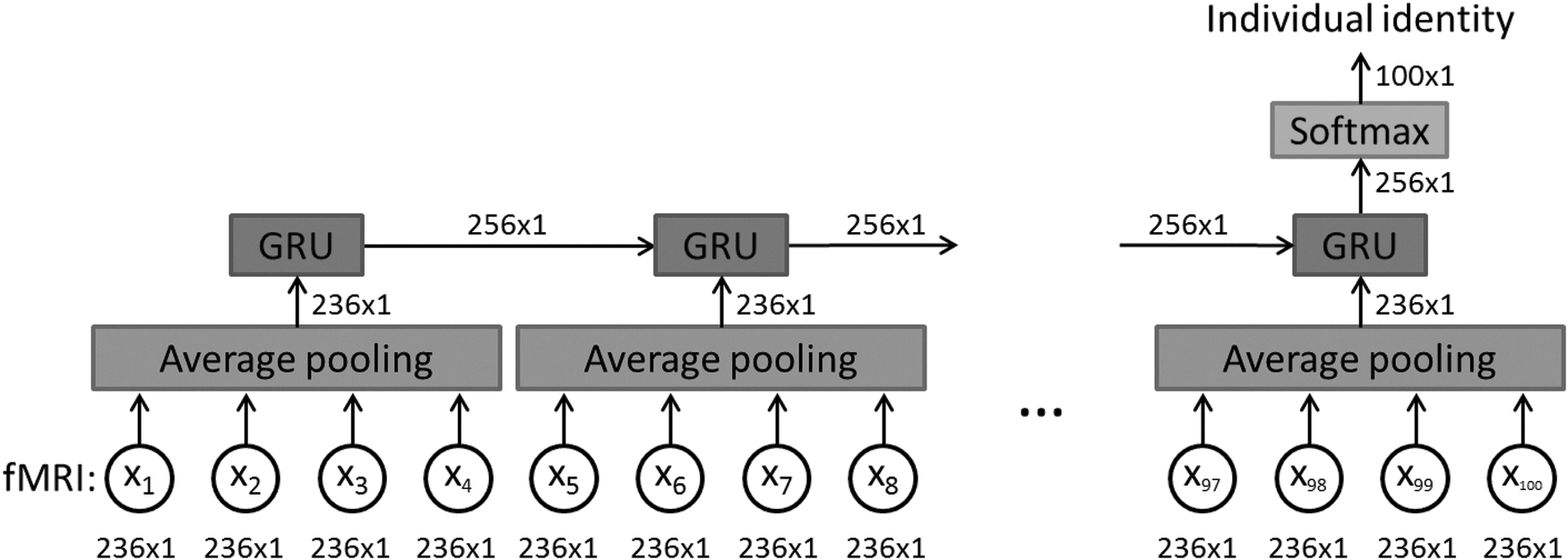
The architecture of our three-layer recurrent neural network-based model. A 25% dropout rate is applied on the input of the average pooling layer as well as the input and recurrent connections of the GRU layer. This figure demonstrates a GRU model unrolled over time. The dimension of data flow through the diagram is also labeled. Note that we assume the input data have 236 regions of interest, so the input data dimension is 236 × 1 at each time step. fMRI, functional magnetic resonance imaging; GRU, gated recurrent unit.
The first layer is an average pooling layer with a length of four on the temporal axis, which means every four time frames are averaged together to generate one output frame. With the input data to this layer being a 236 × 100 matrix with 236 ROIs and 100 time frames, the output of this layer was a 236 × 25 matrix. Reducing the number of time frames from 100 to 25 for the subsequent recurrent layer made computational burden tractable and the model easier to train (Mazumdar and Harley, 2008).
In addition, a 25% dropout was applied on every frame of the input data to alleviate overfitting before the average pooling layer. The dimensions of the data matrix (236 × 25) remained unchanged with the dropout, but 25% of its elements, randomly selected, were set to zero by the dropout.
The second layer is a recurrent layer with 256-dimensional GRU described by the following equations. For simplicity, we will also refer to the 256-dimensional GRU as 256 GRUs:
where at time step t, xt
is the input to the GRU and ht
is the output of the GRU. In Equation (1), the symbol
The softmax layer has an input of 256 dimensions and an output of 100 dimensions. This layer first changes the dimension of the data from 256 to 100 by the multiplication of a weight matrix W. It then maps each dimension of the output to a number between 0 and 1. It also ensures the sum of the 100 dimensions to be 1 as shown in the following equation. Each dimension of the output represents the probability of the input data belonging to the corresponding subject. We have 100 subjects corresponding to 100-dimensional output. Therefore, the one with the largest probability is the model's final prediction of the individual's identity. The loss function for the softmax layer is categorical cross-entropy.
Our recurrent learning model was built using Keras (Chollet, 2015) and trained with Adam optimizer (Kingma and Ba, 2014). The learning rate,
Impact of preprocessing
There is evidence in the literature that the global signal of fMRI during resting state is associated with physiological signals, such as respiration, heart rate, and head motion (Burgess et al., 2016; Power et al., 2017). To test whether our model is sensitive to these kinds of physiological variables, we processed the data both with and without the global signal regression (GSR) and compared the results. We also tested whether our model was sensitive to atlases by extracting the time course using two different atlases with different number of ROIs, as mentioned in the previous subsection.
Results
When predicting individual identity using only 100 time frames (72 sec) of fMRI data, our model was able to achieve 90+% accuracy on validation and testing data. In contrast, functional connectome fingerprint (Finn et al., 2015), which only used FC, achieved <70% accuracy on average. Table 1 shows the accuracy of our model in three different preprocessing approaches (with and without GSR and using two different atlases). A paired t-test between the accuracies of with and without GSR showed that GSR significantly increased test accuracy of data with 236 ROIs (effect size = 0.51, p = 1.37 × 10⁻⁶). A paired t-test between the accuracies using 236 and 360 ROIs, respectively, revealed that changing atlases did not affect the accuracy (effect size = 0.25, p = 0.015) of data with GSR to the same extent.
GSR, global signal regression; ROI, regions of interest.
The output of GRUs is shown in Figure 2. Dots with different colors represent data from different subjects. The output of GRU is a mapping from 256 dimensions to two dimensions by t-distributed stochastic neighbor embedding (Maaten and Hinton, 2008). As shown in the figure, data from different subjects are clustered together in the second layer before going into the final classification layer, which explains the high prediction accuracy. GRU outputs were collected on test datasets, and each subject has around 100 GRU output points.
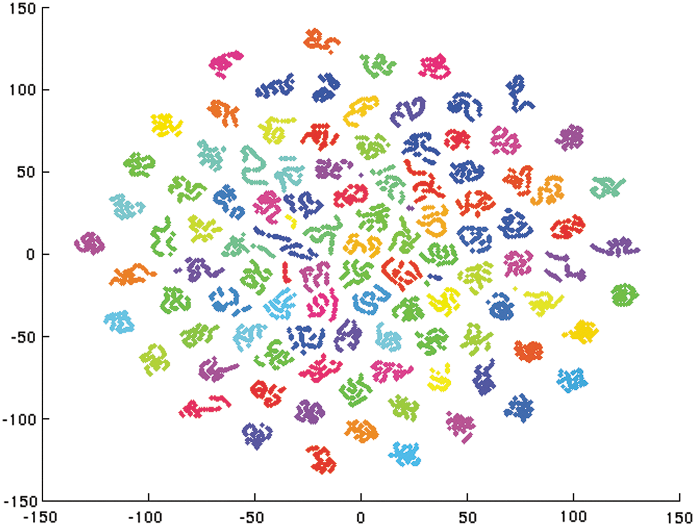
Data from different subjects are clustered as output of the GRU. Dots with different colors are from different subjects. The 256-dimensional output of GRU is visualized in two dimensions by t-distributed stochastic neighbor embedding. Each subject has 100 GRU output points from the test dataset. Color images available online at
Figure 3 shows the output of one GRU of 256 GRUs with respect to different subjects and different time points. Each scan of a subject contains 1200 time frames. Therefore, we used a sliding window approach (window length of 100 time frames; sliding step of one time frame) to generate input to the model. For the input data from each window, the GRUs generated a 256-dimensional output that was fed into the softmax layer. In this study, as an example, we present one dimension of this output and plot the recorded values as a two-dimensional image with subjects and time frames being the two axes. Note that the chosen dimension is the same across all subjects and all time points. The output is between −1 and 1 due to the tanh function applied at the output of GRU. When a GRU is sensitive to the 100 time frames of the input data, the GRU outputs a high absolute value.
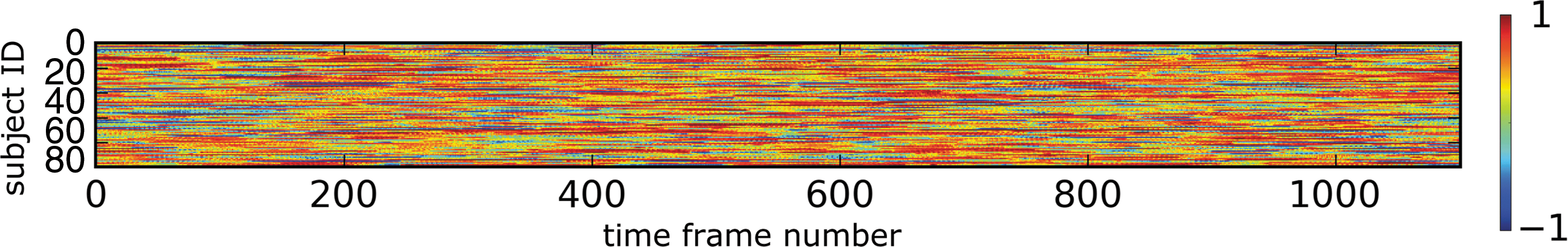
The output of one GRU over time. Each row of the image represents the output of GRU with respect to a different subject. Each column of the image is the output of GRU at a particular time point. Color images available online at
We defined the spatial pattern that each GRU is sensitive to as a GRU pattern, which is a weighted sum of all the raw data time frames in the test dataset. Our resultant GRU patterns are thus at the original resolution rather than just 236 or 360 ROIs as shown in Figure 4. The weights for computing GRU patterns were based on the aforementioned recorded GRU output. Since one GRU output corresponds to 100 time frames of the raw data, each of the 100 time frames gets the same weight, which is equal to the GRU output, and this weight varies between windows when generating GRU output. As a result, the final weights ended up being the moving average (with length of 100) of the recorded GRU output. When computing one GRU pattern, if the weights of one time frame accumulate during the moving average, it means the contribution of this time frame to this GRU adds coherently and should be considered when computing the GRU pattern. These GRU patterns characterize what were captured by GRUs and used as features.
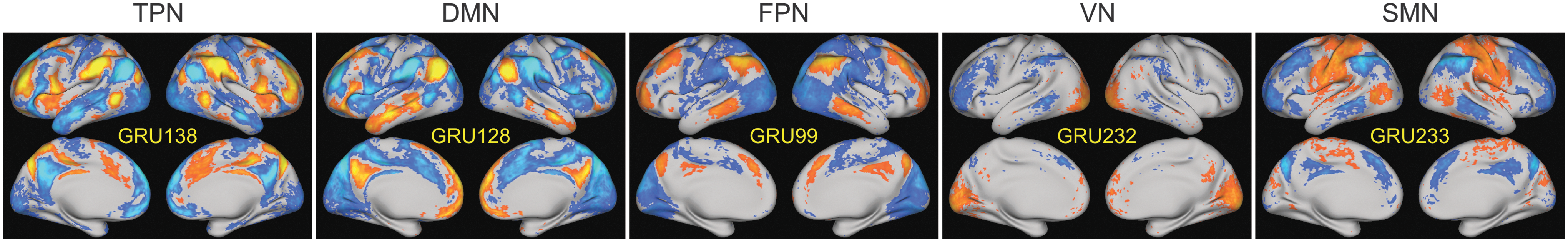
Five representative GRU patterns that resemble five different resting state networks (RSNs). Color images available online at
The resultant 256 GRU patterns resemble resting state networks (RSNs) in the literature (Lee et al., 2013; Yeo et al., 2011). Figure 4 shows five representative GRU patterns averaged over all subjects corresponding to the task-positive network (TPN), default mode network (DMN), frontoparietal network (FPN), visual network (VN), and somatosensory motor network (SMN). We also noticed that variations of one RSN could be captured by multiple GRUs. To cluster similar GRU patterns together and understand the features captured by GRUs in general, we used hierarchical clustering with cosine distance metric and used 0.8 as the threshold for demonstration purpose as shown in Figure 5. The threshold was chosen such that we had some diversity in the resultant clusters and not too many clusters with similar patterns. The cluster centers were computed by averaging all the GRU patterns derived using all subjects in each cluster.
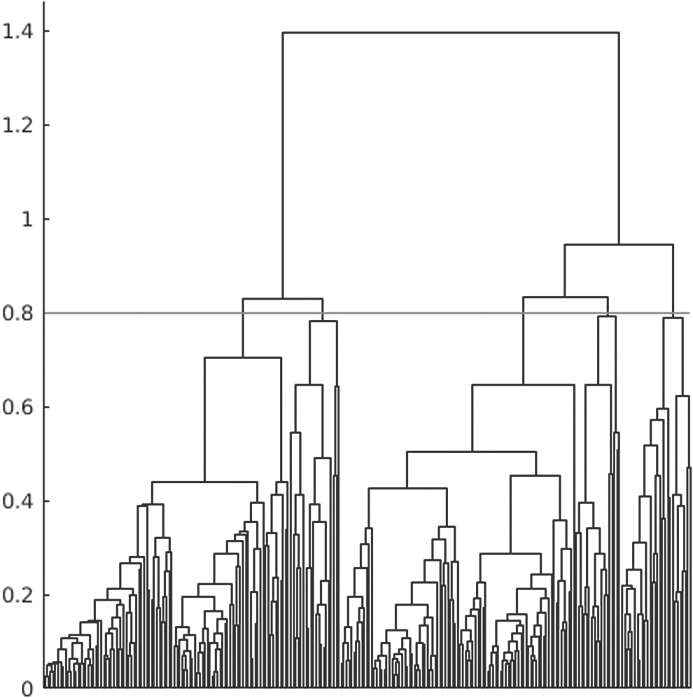
Dendrogram of hierarchical clustering to group 256 GRU patterns into five clusters. The horizontal line indicates the threshold to separate all GRU patterns into clusters.
The same approach was applied on the three differently preprocessed datasets to derive cluster centers of GRU patterns. This resulted in 5, 10, and 8 cluster centers on datasets of 236 ROIs without GSR, 236 ROIs with GSR, and 360 ROIs with GSR as shown in Supplementary Figure S1 (Supplementary Data are available online at
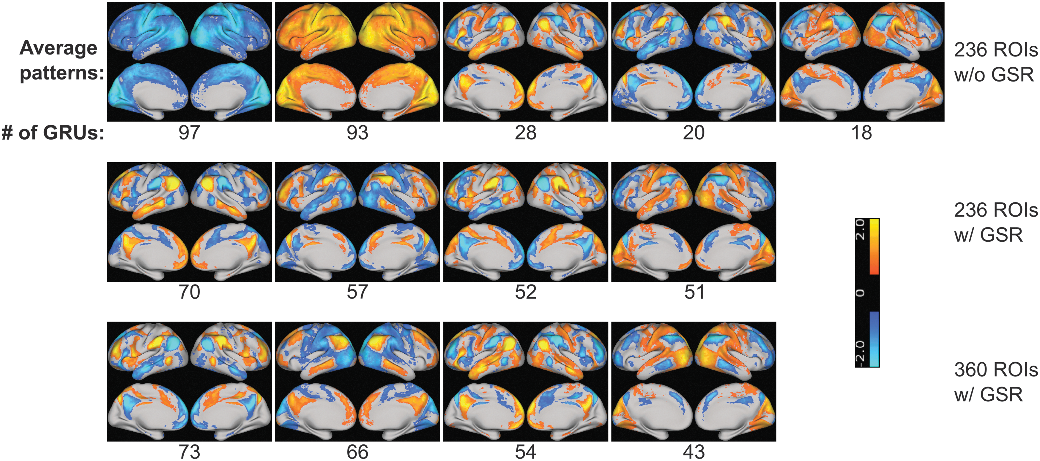
Cluster centers of GRU patterns with three different preprocessing approaches. The number below the image indicates the number of GRU patterns assigned to each cluster. Only clusters with more than 10 GRU patterns are shown here. Color images available online at
We noted that when and only when GSR was not performed, most of the GRUs captured whole-brain deactivation and activation, as shown by the first two images in the first row of Figure 6. In these two whole-brain deactivation/activation images, somatosensory, motor, and visual cortices appear to be the most deactivated/activated. Among all three different preprocessing approaches, positive DMN plus negative TPN (+DMN−TPN) and positive TPN plus negative DMN (+TPN−DMN) are captured by most GRUs. The number of GRUs capturing these two patterns is listed in Table 2. In addition, 18 GRUs detected positive SMN and VN together with negative DMN when GSR was not used. In contrast, 51 and 43 GRUs detected positive SMN and VN plus negative TPN after GSR with 236 and 360 ROIs, respectively. Negative SMN and VN were also captured by GRU after performing GSR. When using 236 ROIs, 57 GRU patterns show negative SMN and VN plus positive TPN, while 66 GRU patterns appear to be negative SMN and VN plus positive DMN when using 360 ROIs.
TPN, task-positive network; DMN, default mode network; +DMN−TPN, DMN plus negative TPN; +TPN−DMN, positive TPN plus negative DMN.
Discussion
A great deal of efforts have been devoted to reducing individual differences using brain templates, volumetric registration, and surface registration (Robinson et al., 2014) so that group-level analysis can be conducted. However, we have shown that individual variability does exist in how the brain functions over time. Given only 72 sec of fMRI data, our recurrent model was able to predict the identity of each individual with 94+% accuracy. The implications of our results are discussed in the following paragraphs.
We have shown that 100 time frames contain sufficient information for individual identification, and our recurrent model outperforms the FC-based approach in individual identification with 72 sec of fMRI data (94% vs. 70%) (Finn et al., 2015). The FC-based approach can be considered as feature selection plus k-nearest neighbor classifier (
Dropout regularization was introduced to deep learning to reduce overfitting by randomly setting some of the input dimensions to zeros while preserving the rest (Srivastava et al., 2014). As a result, it also introduces some duplication in GRU patterns. The more times a pattern is duplicated by the model, the more important this pattern is to identify individuals. In our model, dropout was applied on input layers as well as input and recurrent connections. It forces the model not to rely entirely on one unit if the feature is important, but rather to create multiple copies of the important features with some variations in GRU patterns just in case some GRUs are randomly set to zeros. This explains why many of our GRU patterns are similar. Actually, the number of GRU patterns that show a similar RSN reflects how important that RSN is when deciding the individual identity, that is, how much the final decision relies on a particular GRU pattern.
Although data of all subjects are registered to a template, completely removing their anatomical discrepancy is still difficult. To reduce the anatomical contribution to individual difference, we used the data after volumetric and surface-based registration. The surface registration applied to the HCP data, MSM-ALL, is a multimodal surface matching algorithm, which also considered functional scans. Table 3 shows a substantial decrease in accuracy of the model when switching from resting-state to language task fMRI. This decrease of accuracy suggests that the individual discriminating power is based on brain function rather than brain structure because the brain structure is the same between resting state and language task, and the difference in brain function between resting and task explains the decrease in accuracy. Note that there was no repositioning of the subject between these two scans because the language task and the second resting state scan (REST2) were both acquired on the same day. Several other aspects related to anatomical difference, such as partial volume effect and choice of atlases, are also worth noting.
REST2, second resting state scan; LG, language.
Since training data are from the first day and validation and testing data are from the second day, repositioning of the subject could have led to different partial volume effects. On the other hand, the ROIs we used were 5 mm in radius and would have lessened the partial volume effect. Therefore, the partial volume effect is not a major factor here.
To further understand how the model uses the features to make prediction, we changed the preprocessing steps of input data and examined how different components of the fMRI signal affect GRU patterns and final prediction accuracy. We tested whether or not the model is sensitive to the choice of atlases by using two sets of completely different ROIs. The 236 ROIs are generated based on coordinates of functional nodes from a meta-analysis, and each ROI has a 5-mm radius, which leaves some of the brain region not covered by any ROIs. The 360 ROIs, in contrast, are based on parcellation of the brain, in which all the cortical regions are accounted for. The second and third rows of Table 1 indicate that the difference in atlases did not substantially affect the accuracy. Although the difference is statistically significant (p = 0.015), its effect size is much lower compared with the difference caused by GSR (0.25 vs. 0.51). The second and third rows of Figure 6 show that the features extracted by GRUs are also very similar between the two atlases; they both have +DMN−TPN, +TPN−DMN, and +SMN+VN−TPN patterns. When using 236 ROIs, GRUs tend to capture +TPN−SMN−VN, while with 360 ROIs, GRUs capture +DMN−SMN−VN. Therefore, the change of atlases does affect the GRU patterns a little; however, most of the RSNs captured by GRUs remain the same, and this change does not affect the accuracy greatly.
Physiological effects such as breathing, heartbeat, and head motion affect the fMRI signal (Burgess et al., 2016). For example, the effect of head motion was shown to be consistent across different scans of the same subject and correlated with some behavioral measurements (Siegel et al., 2016). Meanwhile, this physiological signal has also been shown to be correlated with the global signal of fMRI (Power et al., 2017). Therefore, to test whether our model is influenced by physiological effects, we compared the results before and after GSR. If our model is substantially affected by physiological effects, we expect to see a performance decrease after conducting GSR. Although GSR is not guaranteed to eliminate all physiology-related variations, the fact that regressing it out actually increases prediction accuracy suggests that physiological effects are not main contributors to individual identification. In addition, most of the GRU patterns that we derived are significantly correlated with conventional RSNs, as shown in Figure 6. Consequently, the features that are important for individual identification with our model are mostly of neuronal origin. When comparing the GRU patterns derived without GSR and with GSR, the two global activation and deactivation patterns (first two images in the first row of Fig. 6) are similar to the global signal correlation maps reported in literature (Power et al., 2017) where somatosensory, motor, and visual cortices are shown to be most correlated with global signal. This fluctuation in global signal affects the features captured by GRU and thus diminishes the prediction power.
Several limitations of the methodology and additional considerations should be noted. First, although our results suggest that anatomical information is not the main contributor to the individual identification power, volumetric and surface-based registration is not guaranteed to eliminate all anatomical differences. How much of the discriminating power arises from anatomical information needs further investigation. Second, GSR cannot assure the complete removal of physiological effects. In fact, head motion is shown to have a local effect on fMRI signal (Burgess et al., 2016; Siegel et al., 2016). It needs to be further examined how this local effect of the physiological signal can affect the results. Third, although our neural network model has multiple layers, the core of the network is a single layer of GRUs due to the limitation of our computational hardware. Hyperparameter tuning, such as determining the number of layers, the number of units on each layer, and the type of each layer, is still a challenging problem in deep learning. Exhausting all combinations of these parameters and finding the most accurate model are out of the scope of this article. Instead, we are focusing on demonstrating that the RNN-based model can outperform the conventional approach in individual identification and visualizing the features learned by the model. For future directions, we would like to investigate multiple layers of RNNs with different types, such as basic RNN, GRU, and long short-term memory, which can potentially capture more spatiotemporal features of resting-state fMRI data. Finally, from a deep learning perspective, having more layers will enable the model to learn higher level and more complex features. However, understanding and visualizing these high-level features and how the model utilizes these features in the temporal dimension will be intriguing research topics for future directions.
Conclusion
We have applied RNN to individual identification based on resting-state fMRI data. We have demonstrated that 100 time frames (72 sec) are sufficient for training and predicting individual identity. By analyzing data with three different preprocessing approaches, we were able to show that our recurrent model can utilize neuronal information in fMRI data to extract GRU patterns and identify subjects. Therefore, we conclude that the brain functional fingerprints, that is, spatiotemporal features of brain function, can improve our understanding of the uniqueness of each brain.
Footnotes
Author Disclosure Statement
No competing financial interests exist.
References
Supplementary Material
Please find the following supplemental material available below.
For Open Access articles published under a Creative Commons License, all supplemental material carries the same license as the article it is associated with.
For non-Open Access articles published, all supplemental material carries a non-exclusive license, and permission requests for re-use of supplemental material or any part of supplemental material shall be sent directly to the copyright owner as specified in the copyright notice associated with the article.