The use of correlation densities is introduced to quantify and provide visual interpretation for intraregional functional connectivity in the brain. For each brain region, pairwise correlations are computed between a seed voxel and other gray matter voxels within the region, and the distribution of the ensemble of these correlation values is represented as a probability density, the correlation density. The correlation density can be estimated by kernel smoothing. It provides an intuitive and comprehensive representation of subject-specific functional connectivity strength at the local level for each region. To address the challenge of interpreting and utilizing this rich connectivity information when multiple regions are considered, methods from functional data analysis are implemented, including a recently developed method of dimensionality reduction specifically tailored to the analysis of probability distributions. To illustrate the utility of these methods in neuroimaging, experiments were carried out to identify the associations between local functional connectivity and a battery of neurocognitive scores. These experiments demonstrate that correlation densities facilitate the discovery and interpretation of specific region-score associations.
Introduction
The availability of neuroimaging data consisting of time-varying signals across spatial locations in the brain, as provided by functional magnetic resonance imaging (fMRI) or magnetoencephalography and electroencephalography, has made it possible to study functional connectivity, or spatial patterns of time course similarity, in the resting human brain. These patterns are interesting in their own right and have been used for the discovery of the so-called network hubs (Buckner et al., 2009) and other structural properties of brain networks such as small-worldness (Bassett and Bullmore, 2006). An important scientific goal is to relate connectivity to other variables of interest such as age or cognitive status, which conveys external validation that brain connectivity as derived from fMRI is associated with cognitive performance. While various studies have shown the effect of aging on connectivity, a relatively unexplored topic has been to relate, at the individual level, local connectivity patterns with cognitive ability, as measured by cognitive scores. This leads to the challenge of efficiently quantifying local intraregional connectivity as opposed to interregional connectivity, where the latter is a standard topic in connectivity. In this article, we demonstrate a promising approach to achieve such quantification.
Subject-specific connectivity patterns can be investigated on two scales. At the global scale, connections are established by measuring temporal Pearson correlations between summary signals of pairs of brain regions that are spatially far apart and often analyzed using graph-theoretic approaches, after applying a threshold to the Pearson correlations (Achard et al., 2006; Bassett and Bullmore, 2006; Buckner et al., 2009; Tomasi and Volkow, 2011; van den Heuvel et al., 2008; Worsley et al., 2005; Zalesky et al., 2012). At the local scale, correlations between pairs of nearby voxels can be used to quantify the strength of local connectivity of a voxel or local region. Two popular methods for summarizing the strength of this local connectivity are functional connectivity density mapping (Tomasi and Volkow, 2010) and regional homogeneity (Zang et al., 2004). The relevance of local connectivity has been established in a vast number of studies that linked local connectivity patterns to age, gender, and various diseases (Han et al., 2015; Lopez-Larson et al., 2011; Qi et al., 2015; Shukla et al., 2010; Tomasi and Volkow, 2012; Wu et al., 2009; Zalesky et al., 2012).
While intuitive, these current measures of local connectivity sacrifice potentially valuable information as they only represent scalar numeric summaries of a large number of correlations. Another intuitive approach, demonstrated in the study of Petersen and Müller (2016), is to assemble all correlations within a region to obtain a probability density function, the correlation density, for which one can use kernel estimation (Parzen, 1962; Rosenblatt, 1956; Wand and Jones, 1995) or smoothing of histograms (Silverman, 1986). Characteristics such as the mode, spread, and shape of these correlation densities contain potentially valuable information that cannot be quantified by any single numeric summary.
We demonstrate a method to efficiently incorporate information from multiple brain regions to visualize and interpret intraregional connectivity, as well as to investigate associations between local resting-state connectivity and cognitive ability. The proposed approach is based on statistical methodology from functional data analysis (FDA; Ramsay and Silverman, 2005; Wang et al., 2016). The key tool is a recent method of dimensionality reduction specifically tailored to probability density functions (Petersen and Müller, 2016), where it was also shown in an exploratory manner that subject-specific correlation densities for a single region, corresponding to a functional network hub, are useful in predicting executive function test scores. We illustrate the full utility of this approach in connectivity analysis by considering the associations between correlation densities from multiple functional connectivity hubs and a battery of four cognitive test scores, as well as methods of inference and visualization to discover and interpret these associations (Chen et al., 2017). An important point not considered in Petersen and Müller (2016) is that the different correlation densities of a single subject that are associated with different functional connectivity hubs are statistically dependent, so that it is necessary to consider them jointly as predictors in a regression model, implementing appropriate model selection methods. While FDA methods have been utilized previously in functional connectivity studies (Bassett et al., 2012; Hosseini et al., 2012), another important aspect of the approach studied here is the use of subject-specific connectivity information, rather than the usual group-based approach, where one works with averages across the subjects belonging to a group.
Materials and Methods
Participants, fMRI acquisition, and preprocessing
The example data used here to demonstrate our methods are from a study of elderly participants in a longitudinal study of cognitive impairment that has been described previously in Hinton et al. (2010). Participants were evaluated within the research program of the University of California, Davis Alzheimer's Disease Center, as described in He et al. (2012), where also a description of the clinical evaluation of this cohort and the neuropsychological test battery is provided. Included in our analyses are a group of 164 cognitively normal subjects and a second group of 63 subjects diagnosed with Alzheimer's disease.
As described previously (He et al., 2012), fMRI scans were performed at the University of California Davis Imaging Research Center on a 1.5 T GE Signa Horizon LX Echospeed system, along with an 8-min axial echo-planar imaging blood oxygen-level dependent (BOLD) fMRI scan. Subjects were provided with no specific instructions before the acquisition other than to keep their eyes open. The scan parameters were as follows: repetition time (TR) 2.0 s, echo time (TE) 40 ms, field of view (FOV) 22 cm, flip angle 90°, 24 five-millimeter-thick contiguous slices with bandwidth 62.5 KHz, and 64 × 64 matrix with R-L frequency encode direction. This sequence provided 240 time points of data at each voxel.
The standard preprocessing steps of slice timing and head motion correction, followed by coregistration to the subject's 3DT1 MRI scan, were performed. Multiple linear regression was applied to the signal at each voxel to remove global linear trends to account for signal drift, as well as global cerebral spinal fluid and white matter signals. Finally, a band-pass filter was applied, preserving frequency components between 0.01 and 0.08 Hz. These steps were performed in MATLAB, using the Statistical Parametric Mapping (SPM8, www.fil.ion.ucl.ac.uk/spm) and Resting-State fMRI Data Analysis Toolkit V1.8 (REST1.8, http://restfmri.net/forum/?q=rest). The first four time points were discarded to eliminate nonequilibrium effects of magnetization. Time points with large head motion, defined as translation >1.5 mm and/or rotation >1.5°, were then identified, and participants with any such time points were excluded.
Functional principal component analysis
The statistical analysis of a random sample \documentclass{aastex}\usepackage{amsbsy}\usepackage{amsfonts}\usepackage{amssymb}\usepackage{bm}\usepackage{mathrsfs}\usepackage{pifont}\usepackage{stmaryrd}\usepackage{textcomp}\usepackage{portland, xspace}\usepackage{amsmath, amsxtra}\usepackage{upgreek}\pagestyle{empty}\DeclareMathSizes{10}{9}{7}{6}\begin{document}$${X_1} , \ldots , {X_n}$$ \end{document}, where \documentclass{aastex}\usepackage{amsbsy}\usepackage{amsfonts}\usepackage{amssymb}\usepackage{bm}\usepackage{mathrsfs}\usepackage{pifont}\usepackage{stmaryrd}\usepackage{textcomp}\usepackage{portland, xspace}\usepackage{amsmath, amsxtra}\usepackage{upgreek}\pagestyle{empty}\DeclareMathSizes{10}{9}{7}{6}\begin{document}$${X_i}: [ 0 , 1 ] \to \mathbb{R}$$ \end{document} are functions with a common domain, is known as FDA (Ramsay and Silverman, 2005; Wang et al., 2016), or simply FDA. Due to the infinite dimensionality of function spaces, dimension reduction is a key FDA technique. Many FDA methodologies rely on the Karhunen–Loève expansion\documentclass{aastex}\usepackage{amsbsy}\usepackage{amsfonts}\usepackage{amssymb}\usepackage{bm}\usepackage{mathrsfs}\usepackage{pifont}\usepackage{stmaryrd}\usepackage{textcomp}\usepackage{portland, xspace}\usepackage{amsmath, amsxtra}\usepackage{upgreek}\pagestyle{empty}\DeclareMathSizes{10}{9}{7}{6}\begin{document} \begin{align*}{X_i} ( t ) = \mu ( t ) + \sum \nolimits_{k = 1}^ \infty { \xi _{ik}}{ \phi _k} ( t ) , \tag{1} \end{align*} \end{document}
where \documentclass{aastex}\usepackage{amsbsy}\usepackage{amsfonts}\usepackage{amssymb}\usepackage{bm}\usepackage{mathrsfs}\usepackage{pifont}\usepackage{stmaryrd}\usepackage{textcomp}\usepackage{portland, xspace}\usepackage{amsmath, amsxtra}\usepackage{upgreek}\pagestyle{empty}\DeclareMathSizes{10}{9}{7}{6}\begin{document}$$\mu ( t ) = E ( X ( t ) )$$ \end{document} is the mean function, \documentclass{aastex}\usepackage{amsbsy}\usepackage{amsfonts}\usepackage{amssymb}\usepackage{bm}\usepackage{mathrsfs}\usepackage{pifont}\usepackage{stmaryrd}\usepackage{textcomp}\usepackage{portland, xspace}\usepackage{amsmath, amsxtra}\usepackage{upgreek}\pagestyle{empty}\DeclareMathSizes{10}{9}{7}{6}\begin{document}$${ \phi _k}$$ \end{document} are eigenfunctions associated with the covariance kernel \documentclass{aastex}\usepackage{amsbsy}\usepackage{amsfonts}\usepackage{amssymb}\usepackage{bm}\usepackage{mathrsfs}\usepackage{pifont}\usepackage{stmaryrd}\usepackage{textcomp}\usepackage{portland, xspace}\usepackage{amsmath, amsxtra}\usepackage{upgreek}\pagestyle{empty}\DeclareMathSizes{10}{9}{7}{6}\begin{document}$$G ( s , t ) = E \left[ { \left( {{X_i} ( s ) - \mu ( s ) } \right) {X_i} ( t ) } \right]$$ \end{document} with corresponding eigenvalues \documentclass{aastex}\usepackage{amsbsy}\usepackage{amsfonts}\usepackage{amssymb}\usepackage{bm}\usepackage{mathrsfs}\usepackage{pifont}\usepackage{stmaryrd}\usepackage{textcomp}\usepackage{portland, xspace}\usepackage{amsmath, amsxtra}\usepackage{upgreek}\pagestyle{empty}\DeclareMathSizes{10}{9}{7}{6}\begin{document}$${ \lambda _1} \ge { \lambda _2} \ge \cdots \ge 0$$ \end{document}, and\documentclass{aastex}\usepackage{amsbsy}\usepackage{amsfonts}\usepackage{amssymb}\usepackage{bm}\usepackage{mathrsfs}\usepackage{pifont}\usepackage{stmaryrd}\usepackage{textcomp}\usepackage{portland, xspace}\usepackage{amsmath, amsxtra}\usepackage{upgreek}\pagestyle{empty}\DeclareMathSizes{10}{9}{7}{6}\begin{document} \begin{align*}{ \xi _{ik}} = \int_0^1 ( {X_i} ( t ) - \mu ( t ) ) { \phi _k} ( t ) \;{ \rm{dt}} \tag{2} \end{align*} \end{document}
are the uncorrelated functional principal component (FPC) scores with mean 0 and variance \documentclass{aastex}\usepackage{amsbsy}\usepackage{amsfonts}\usepackage{amssymb}\usepackage{bm}\usepackage{mathrsfs}\usepackage{pifont}\usepackage{stmaryrd}\usepackage{textcomp}\usepackage{portland, xspace}\usepackage{amsmath, amsxtra}\usepackage{upgreek}\pagestyle{empty}\DeclareMathSizes{10}{9}{7}{6}\begin{document}$${ \lambda _k}.$$ \end{document} Expansion (Equation 1) provides a linear representation of the data, the functional principal component analysis (FPCA). These representations are the infinite-dimensional analog of principal components analysis (PCA) for multivariate data.
Dimensionality reduction is then obtained by truncating the sum to a finite number of components, as well as visualization of the average behavior of the process via the mean function \documentclass{aastex}\usepackage{amsbsy}\usepackage{amsfonts}\usepackage{amssymb}\usepackage{bm}\usepackage{mathrsfs}\usepackage{pifont}\usepackage{stmaryrd}\usepackage{textcomp}\usepackage{portland, xspace}\usepackage{amsmath, amsxtra}\usepackage{upgreek}\pagestyle{empty}\DeclareMathSizes{10}{9}{7}{6}\begin{document}$$\mu$$ \end{document} and the dominant modes of variation \documentclass{aastex}\usepackage{amsbsy}\usepackage{amsfonts}\usepackage{amssymb}\usepackage{bm}\usepackage{mathrsfs}\usepackage{pifont}\usepackage{stmaryrd}\usepackage{textcomp}\usepackage{portland, xspace}\usepackage{amsmath, amsxtra}\usepackage{upgreek}\pagestyle{empty}\DeclareMathSizes{10}{9}{7}{6}\begin{document}$$\mu \pm \alpha { \phi _k}$$ \end{document} (Jones and Rice, 1992), which lend interpretability to the scores \documentclass{aastex}\usepackage{amsbsy}\usepackage{amsfonts}\usepackage{amssymb}\usepackage{bm}\usepackage{mathrsfs}\usepackage{pifont}\usepackage{stmaryrd}\usepackage{textcomp}\usepackage{portland, xspace}\usepackage{amsmath, amsxtra}\usepackage{upgreek}\pagestyle{empty}\DeclareMathSizes{10}{9}{7}{6}\begin{document}$${ \xi _{ik}}.$$ \end{document}
Functional data analysis for density functions
To perform dimension reduction for a sample of univariate probability distributions, which are often best represented and visualized through their density functions \documentclass{aastex}\usepackage{amsbsy}\usepackage{amsfonts}\usepackage{amssymb}\usepackage{bm}\usepackage{mathrsfs}\usepackage{pifont}\usepackage{stmaryrd}\usepackage{textcomp}\usepackage{portland, xspace}\usepackage{amsmath, amsxtra}\usepackage{upgreek}\pagestyle{empty}\DeclareMathSizes{10}{9}{7}{6}\begin{document}$${f_1} , \ldots , {f_n}$$ \end{document}, direct application of standard FDA methodology (Kneip and Utikal, 2001) has proven suboptimal (Petersen and Müller, 2016). This is due to the nonlinearity of the space of densities implied by the constraints that a density be positive and integrate to one. A more promising approach is to transform the densities into a Hilbert space via a nonlinear functional transformation \documentclass{aastex}\usepackage{amsbsy}\usepackage{amsfonts}\usepackage{amssymb}\usepackage{bm}\usepackage{mathrsfs}\usepackage{pifont}\usepackage{stmaryrd}\usepackage{textcomp}\usepackage{portland, xspace}\usepackage{amsmath, amsxtra}\usepackage{upgreek}\pagestyle{empty}\DeclareMathSizes{10}{9}{7}{6}\begin{document}$$\psi$$ \end{document}, yielding a sample \documentclass{aastex}\usepackage{amsbsy}\usepackage{amsfonts}\usepackage{amssymb}\usepackage{bm}\usepackage{mathrsfs}\usepackage{pifont}\usepackage{stmaryrd}\usepackage{textcomp}\usepackage{portland, xspace}\usepackage{amsmath, amsxtra}\usepackage{upgreek}\pagestyle{empty}\DeclareMathSizes{10}{9}{7}{6}\begin{document}$${X_i} = \psi ( {f_i} )$$ \end{document}, to which the standard FDA methodology can then be suitably applied, as the transformed functions are not subject to any restrictions.
To illustrate the utility of such a nonlinear transformation, consider a basic setup in finite dimensions. Here, one observes\documentclass{aastex}\usepackage{amsbsy}\usepackage{amsfonts}\usepackage{amssymb}\usepackage{bm}\usepackage{mathrsfs}\usepackage{pifont}\usepackage{stmaryrd}\usepackage{textcomp}\usepackage{portland, xspace}\usepackage{amsmath, amsxtra}\usepackage{upgreek}\pagestyle{empty}\DeclareMathSizes{10}{9}{7}{6}\begin{document} \begin{align*}{Y_i} = ( \sin ( {Z_{i1}} + {Z_{i2}} ) , \cos ( {Z_{i1}} - {Z_{i2}} ) ) , \end{align*} \end{document}
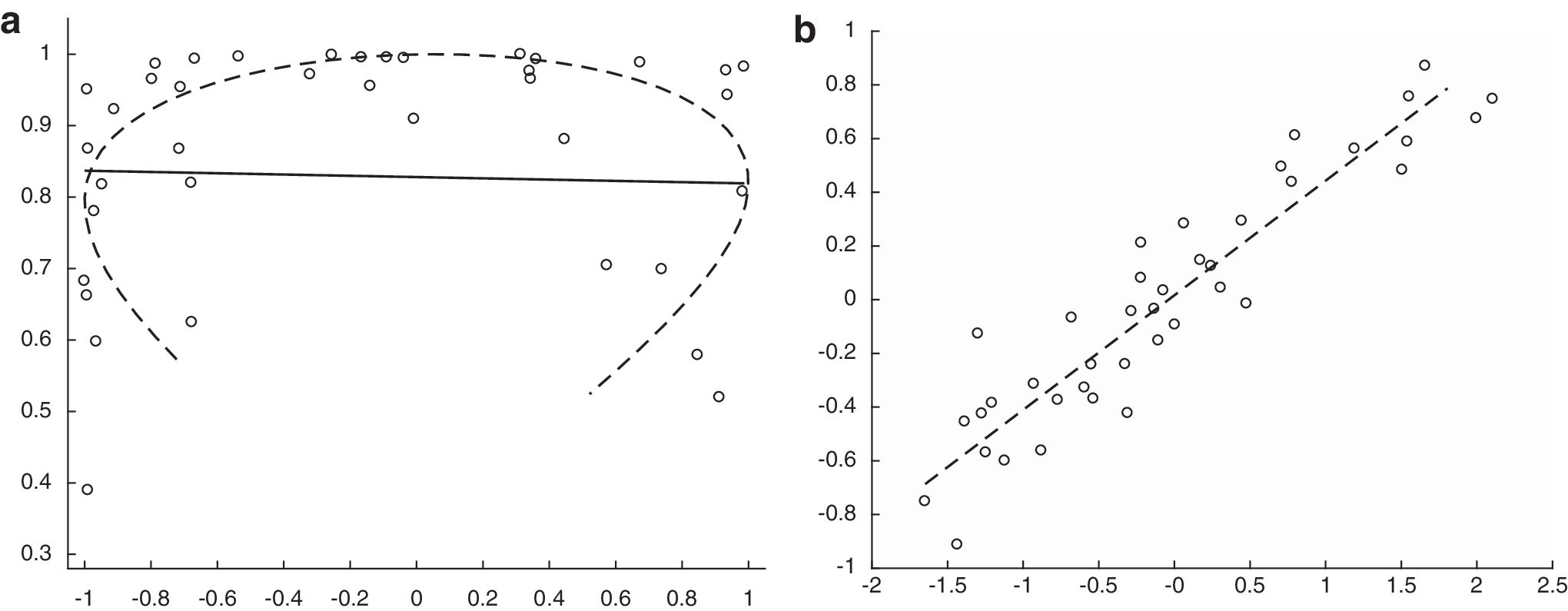
where \documentclass{aastex}\usepackage{amsbsy}\usepackage{amsfonts}\usepackage{amssymb}\usepackage{bm}\usepackage{mathrsfs}\usepackage{pifont}\usepackage{stmaryrd}\usepackage{textcomp}\usepackage{portland, xspace}\usepackage{amsmath, amsxtra}\usepackage{upgreek}\pagestyle{empty}\DeclareMathSizes{10}{9}{7}{6}\begin{document}$${Z_i} = ( {Z_{i1}} , {Z_{i2}} )$$ \end{document} are a bivariate normal sample with \documentclass{aastex}\usepackage{amsbsy}\usepackage{amsfonts}\usepackage{amssymb}\usepackage{bm}\usepackage{mathrsfs}\usepackage{pifont}\usepackage{stmaryrd}\usepackage{textcomp}\usepackage{portland, xspace}\usepackage{amsmath, amsxtra}\usepackage{upgreek}\pagestyle{empty}\DeclareMathSizes{10}{9}{7}{6}\begin{document}$${ \rm{Var}} ( {Z_{i1}} ) = 1$$ \end{document}, \documentclass{aastex}\usepackage{amsbsy}\usepackage{amsfonts}\usepackage{amssymb}\usepackage{bm}\usepackage{mathrsfs}\usepackage{pifont}\usepackage{stmaryrd}\usepackage{textcomp}\usepackage{portland, xspace}\usepackage{amsmath, amsxtra}\usepackage{upgreek}\pagestyle{empty}\DeclareMathSizes{10}{9}{7}{6}\begin{document}$${ \rm{Var}} ( {Z_{i2}} ) = 0.2$$ \end{document} and correlation 0.95. Figure 1a shows the data and the first PCA direction (i.e., the orthogonal least squares line) for a sample \documentclass{aastex}\usepackage{amsbsy}\usepackage{amsfonts}\usepackage{amssymb}\usepackage{bm}\usepackage{mathrsfs}\usepackage{pifont}\usepackage{stmaryrd}\usepackage{textcomp}\usepackage{portland, xspace}\usepackage{amsmath, amsxtra}\usepackage{upgreek}\pagestyle{empty}\DeclareMathSizes{10}{9}{7}{6}\begin{document}$${Y_1} , \ldots , {Y_{40}}$$ \end{document}, which is clearly unsatisfactory due to the nonlinear nature of data. Alternatively, one can transform the data and obtain the first PCA loading (orthogonal least squares line) of the Gaussian data \documentclass{aastex}\usepackage{amsbsy}\usepackage{amsfonts}\usepackage{amssymb}\usepackage{bm}\usepackage{mathrsfs}\usepackage{pifont}\usepackage{stmaryrd}\usepackage{textcomp}\usepackage{portland, xspace}\usepackage{amsmath, amsxtra}\usepackage{upgreek}\pagestyle{empty}\DeclareMathSizes{10}{9}{7}{6}\begin{document}$${Z_1} , \ldots , {Z_{40}}$$ \end{document} (Fig. 1b), which is appropriate due to the linear nature of these data, and then map it back to the original space, obtaining the curved dashed line in Figure 1a, and thus a much more informative analysis.
(a) Scatter plot of nonlinear data Yi, with linear PCA loading (orthogonal least squares; solid line) and nonlinear loading (dashed line) obtained by transforming the loading obtained for the data Zi. (b) Original data Zi with the first PCA loading (orthogonal least squares; dashed line). PCA, principal component analysis.
Of course, in the case of density functions, one cannot so easily transform the densities so that the transformed versions have a known distribution, such as a Gaussian process. However, Petersen and Müller (2016) discussed several generic transformations that transform density functions into unrestricted square integrable functions and thus improve upon the naive FPCA directly applied to the density functions. The most promising transformation utilizes the so-called quantile density function \documentclass{aastex}\usepackage{amsbsy}\usepackage{amsfonts}\usepackage{amssymb}\usepackage{bm}\usepackage{mathrsfs}\usepackage{pifont}\usepackage{stmaryrd}\usepackage{textcomp}\usepackage{portland, xspace}\usepackage{amsmath, amsxtra}\usepackage{upgreek}\pagestyle{empty}\DeclareMathSizes{10}{9}{7}{6}\begin{document}$$q ( t ) = Q \prime ( t )$$ \end{document}, where Q is the quantile function corresponding to a density f. The log-quantile density (LQD) transformation of f is\documentclass{aastex}\usepackage{amsbsy}\usepackage{amsfonts}\usepackage{amssymb}\usepackage{bm}\usepackage{mathrsfs}\usepackage{pifont}\usepackage{stmaryrd}\usepackage{textcomp}\usepackage{portland, xspace}\usepackage{amsmath, amsxtra}\usepackage{upgreek}\pagestyle{empty}\DeclareMathSizes{10}{9}{7}{6}\begin{document} \begin{align*} X ( t ) = \psi ( f ) ( t ) = \log ( q ( t ) ) = - \log ( \,f ( Q ( t ) ) ) , \quad t \in [ 0 , 1 ]. \tag{3} \end{align*} \end{document}
If one starts with a sample \documentclass{aastex}\usepackage{amsbsy}\usepackage{amsfonts}\usepackage{amssymb}\usepackage{bm}\usepackage{mathrsfs}\usepackage{pifont}\usepackage{stmaryrd}\usepackage{textcomp}\usepackage{portland, xspace}\usepackage{amsmath, amsxtra}\usepackage{upgreek}\pagestyle{empty}\DeclareMathSizes{10}{9}{7}{6}\begin{document}$${f_1} , \ldots , {f_n}$$ \end{document} of density functions, this transformation then gives rise to a sample of unrestricted square integrable functions \documentclass{aastex}\usepackage{amsbsy}\usepackage{amsfonts}\usepackage{amssymb}\usepackage{bm}\usepackage{mathrsfs}\usepackage{pifont}\usepackage{stmaryrd}\usepackage{textcomp}\usepackage{portland, xspace}\usepackage{amsmath, amsxtra}\usepackage{upgreek}\pagestyle{empty}\DeclareMathSizes{10}{9}{7}{6}\begin{document}$${X_1} , \ldots {X_n}$$ \end{document} on the domain \documentclass{aastex}\usepackage{amsbsy}\usepackage{amsfonts}\usepackage{amssymb}\usepackage{bm}\usepackage{mathrsfs}\usepackage{pifont}\usepackage{stmaryrd}\usepackage{textcomp}\usepackage{portland, xspace}\usepackage{amsmath, amsxtra}\usepackage{upgreek}\pagestyle{empty}\DeclareMathSizes{10}{9}{7}{6}\begin{document}$$[ 0 , 1 ]$$ \end{document}, for which all available FDA methods can be applied, including functional regression or FPCA. By computing the elements of the decomposition in Equation 1, the dominant modes of variation are most usefully visualized as densities by means of the inverse transformation. The transformation modes are obtained across a range of values α as\documentclass{aastex}\usepackage{amsbsy}\usepackage{amsfonts}\usepackage{amssymb}\usepackage{bm}\usepackage{mathrsfs}\usepackage{pifont}\usepackage{stmaryrd}\usepackage{textcomp}\usepackage{portland, xspace}\usepackage{amsmath, amsxtra}\usepackage{upgreek}\pagestyle{empty}\DeclareMathSizes{10}{9}{7}{6}\begin{document} \begin{align*}{ \psi ^{ - 1}} \left( { \mu \pm \alpha { \phi _j}} \right). \tag{4} \end{align*} \end{document}
Quantifying intraregional connectivity by correlation densities
Our experiments focused on the intraregional connectivity properties of 10 functional hubs, which are listed together with their seed voxels in the study of Buckner et al. (2009; see table 3 therein) and correspond to the following regions: left/right parietal lobules (LPL/RPL), left/right middle frontal (LMF/RMF), left/right middle temporal (LMT/RMT), medial superior frontal (MSF), medial prefrontal (MP), posterior cingulate/precuneus (PCP), and right supramarginal (RS). Since only the seed voxels, and not the region boundaries, were well defined, we took the following approach to construct the correlation density for each region at the subject level. First, for a given region, an \documentclass{aastex}\usepackage{amsbsy}\usepackage{amsfonts}\usepackage{amssymb}\usepackage{bm}\usepackage{mathrsfs}\usepackage{pifont}\usepackage{stmaryrd}\usepackage{textcomp}\usepackage{portland, xspace}\usepackage{amsmath, amsxtra}\usepackage{upgreek}\pagestyle{empty}\DeclareMathSizes{10}{9}{7}{6}\begin{document}$$11 \times 11 \times 11$$ \end{document} cube of voxels was isolated, centered at the seed voxel, and a mask was then used to extract the signals of all gray matter voxels within this cube. Second, letting m be the number of identified gray matter voxels including the seed voxel, the preprocessed fMRI signals for each were used to obtain pairwise Pearson correlations \documentclass{aastex}\usepackage{amsbsy}\usepackage{amsfonts}\usepackage{amssymb}\usepackage{bm}\usepackage{mathrsfs}\usepackage{pifont}\usepackage{stmaryrd}\usepackage{textcomp}\usepackage{portland, xspace}\usepackage{amsmath, amsxtra}\usepackage{upgreek}\pagestyle{empty}\DeclareMathSizes{10}{9}{7}{6}\begin{document}$${ \rho _k} ,$$ \end{document}\documentclass{aastex}\usepackage{amsbsy}\usepackage{amsfonts}\usepackage{amssymb}\usepackage{bm}\usepackage{mathrsfs}\usepackage{pifont}\usepackage{stmaryrd}\usepackage{textcomp}\usepackage{portland, xspace}\usepackage{amsmath, amsxtra}\usepackage{upgreek}\pagestyle{empty}\DeclareMathSizes{10}{9}{7}{6}\begin{document}$$k = 1 , \ldots , m - 1$$ \end{document}, between the seed voxel signal and the remaining \documentclass{aastex}\usepackage{amsbsy}\usepackage{amsfonts}\usepackage{amssymb}\usepackage{bm}\usepackage{mathrsfs}\usepackage{pifont}\usepackage{stmaryrd}\usepackage{textcomp}\usepackage{portland, xspace}\usepackage{amsmath, amsxtra}\usepackage{upgreek}\pagestyle{empty}\DeclareMathSizes{10}{9}{7}{6}\begin{document}$$m - 1$$ \end{document} gray matter signals. Alternative similarity measures besides Pearson correlation could also be used. As a final step, only gray matter voxels for which \documentclass{aastex}\usepackage{amsbsy}\usepackage{amsfonts}\usepackage{amssymb}\usepackage{bm}\usepackage{mathrsfs}\usepackage{pifont}\usepackage{stmaryrd}\usepackage{textcomp}\usepackage{portland, xspace}\usepackage{amsmath, amsxtra}\usepackage{upgreek}\pagestyle{empty}\DeclareMathSizes{10}{9}{7}{6}\begin{document}$${ \rho _k}$$ \end{document} is positive are considered to be part of the corresponding region, so that negative correlations are effectively discarded.
The elimination of negative correlations is similar to other approaches in the analysis of local functional connectivity (Tomasi and Volkow, 2010) and is also in line with the study of Craddock et al. (2012), which specified functional regions of interest as “spatially coherent regions of homogeneous functional connectivity.” Moreover, we found that negative correlations were rare for voxels nearby the seed voxel and mostly concentrated on the boundary of the cube.
The correlation density for a specific region and a specific individual is then defined as the probability density function of the distribution of the correlations \documentclass{aastex}\usepackage{amsbsy}\usepackage{amsfonts}\usepackage{amssymb}\usepackage{bm}\usepackage{mathrsfs}\usepackage{pifont}\usepackage{stmaryrd}\usepackage{textcomp}\usepackage{portland, xspace}\usepackage{amsmath, amsxtra}\usepackage{upgreek}\pagestyle{empty}\DeclareMathSizes{10}{9}{7}{6}\begin{document}$${ \rho _k}$$ \end{document} that are positive. The domain of the correlation densities is the interval \documentclass{aastex}\usepackage{amsbsy}\usepackage{amsfonts}\usepackage{amssymb}\usepackage{bm}\usepackage{mathrsfs}\usepackage{pifont}\usepackage{stmaryrd}\usepackage{textcomp}\usepackage{portland, xspace}\usepackage{amsmath, amsxtra}\usepackage{upgreek}\pagestyle{empty}\DeclareMathSizes{10}{9}{7}{6}\begin{document}$$[ 0 , 1 ]$$ \end{document}. The estimated correlation densities \documentclass{aastex}\usepackage{amsbsy}\usepackage{amsfonts}\usepackage{amssymb}\usepackage{bm}\usepackage{mathrsfs}\usepackage{pifont}\usepackage{stmaryrd}\usepackage{textcomp}\usepackage{portland, xspace}\usepackage{amsmath, amsxtra}\usepackage{upgreek}\pagestyle{empty}\DeclareMathSizes{10}{9}{7}{6}\begin{document}$${f_{ij}}$$ \end{document}, \documentclass{aastex}\usepackage{amsbsy}\usepackage{amsfonts}\usepackage{amssymb}\usepackage{bm}\usepackage{mathrsfs}\usepackage{pifont}\usepackage{stmaryrd}\usepackage{textcomp}\usepackage{portland, xspace}\usepackage{amsmath, amsxtra}\usepackage{upgreek}\pagestyle{empty}\DeclareMathSizes{10}{9}{7}{6}\begin{document}$$i = 1 , \ldots , n ,$$ \end{document}\documentclass{aastex}\usepackage{amsbsy}\usepackage{amsfonts}\usepackage{amssymb}\usepackage{bm}\usepackage{mathrsfs}\usepackage{pifont}\usepackage{stmaryrd}\usepackage{textcomp}\usepackage{portland, xspace}\usepackage{amsmath, amsxtra}\usepackage{upgreek}\pagestyle{empty}\DeclareMathSizes{10}{9}{7}{6}\begin{document}$$j = 1 , \ldots , 10$$ \end{document}, for each of n subjects are obtained from the sample of correlations for the jth region by applying a density estimation method, such as kernel density estimation (Rosenblatt, 1956) or smoothing histograms (Petersen and Müller, 2016). The correlation densities provide useful visualizations of intraregional connectivity, for each region considered and each individual in the sample (see the Results section).
Once the correlation densities \documentclass{aastex}\usepackage{amsbsy}\usepackage{amsfonts}\usepackage{amssymb}\usepackage{bm}\usepackage{mathrsfs}\usepackage{pifont}\usepackage{stmaryrd}\usepackage{textcomp}\usepackage{portland, xspace}\usepackage{amsmath, amsxtra}\usepackage{upgreek}\pagestyle{empty}\DeclareMathSizes{10}{9}{7}{6}\begin{document}$${f_{ij}}$$ \end{document} have been obtained, we apply transformations (Equation 3) to obtain corresponding unrestricted functions \documentclass{aastex}\usepackage{amsbsy}\usepackage{amsfonts}\usepackage{amssymb}\usepackage{bm}\usepackage{mathrsfs}\usepackage{pifont}\usepackage{stmaryrd}\usepackage{textcomp}\usepackage{portland, xspace}\usepackage{amsmath, amsxtra}\usepackage{upgreek}\pagestyle{empty}\DeclareMathSizes{10}{9}{7}{6}\begin{document}$${X_{ij}}$$ \end{document} and then FPCA for dimension reduction, applying (Equation 1) and truncating the expansion at Kj expansion terms. Here, we select Kj so that 95% of the variation in the functions \documentclass{aastex}\usepackage{amsbsy}\usepackage{amsfonts}\usepackage{amssymb}\usepackage{bm}\usepackage{mathrsfs}\usepackage{pifont}\usepackage{stmaryrd}\usepackage{textcomp}\usepackage{portland, xspace}\usepackage{amsmath, amsxtra}\usepackage{upgreek}\pagestyle{empty}\DeclareMathSizes{10}{9}{7}{6}\begin{document}$${X_{ij}}$$ \end{document} across individuals are explained. This dimension reduction step then results in a vector of dimension Kj of FPCs that represent the functions \documentclass{aastex}\usepackage{amsbsy}\usepackage{amsfonts}\usepackage{amssymb}\usepackage{bm}\usepackage{mathrsfs}\usepackage{pifont}\usepackage{stmaryrd}\usepackage{textcomp}\usepackage{portland, xspace}\usepackage{amsmath, amsxtra}\usepackage{upgreek}\pagestyle{empty}\DeclareMathSizes{10}{9}{7}{6}\begin{document}$${X_{ij}}$$ \end{document} for each individual and thus the correlation densities \documentclass{aastex}\usepackage{amsbsy}\usepackage{amsfonts}\usepackage{amssymb}\usepackage{bm}\usepackage{mathrsfs}\usepackage{pifont}\usepackage{stmaryrd}\usepackage{textcomp}\usepackage{portland, xspace}\usepackage{amsmath, amsxtra}\usepackage{upgreek}\pagestyle{empty}\DeclareMathSizes{10}{9}{7}{6}\begin{document}$${f_{ij}}$$ \end{document}. These vectors can then be used as components of various statistical models, for example, as predictors in a regression model. We demonstrate this approach in the Results section.
Correlation densities as predictors in a functional linear model
We aim here at regression models, where the subject-specific vectors of FPCs of the transformed density functions for the regions considered are the predictors and the responses are the cognitive scores. This allows to quantify the relations between subject-specific intraregional connectivities and cognitive performance. Specifically, in the Results section, we utilize a subject's local connectivity characteristics, as quantified by the distributions of correlations for several brain regions, to predict each of four scalar cognitive scores. If J distinct regions are considered for n subjects in a sample, our regression model features predictors \documentclass{aastex}\usepackage{amsbsy}\usepackage{amsfonts}\usepackage{amssymb}\usepackage{bm}\usepackage{mathrsfs}\usepackage{pifont}\usepackage{stmaryrd}\usepackage{textcomp}\usepackage{portland, xspace}\usepackage{amsmath, amsxtra}\usepackage{upgreek}\pagestyle{empty}\DeclareMathSizes{10}{9}{7}{6}\begin{document}$${f_{ij}}$$ \end{document}, \documentclass{aastex}\usepackage{amsbsy}\usepackage{amsfonts}\usepackage{amssymb}\usepackage{bm}\usepackage{mathrsfs}\usepackage{pifont}\usepackage{stmaryrd}\usepackage{textcomp}\usepackage{portland, xspace}\usepackage{amsmath, amsxtra}\usepackage{upgreek}\pagestyle{empty}\DeclareMathSizes{10}{9}{7}{6}\begin{document}$$i = 1 , \ldots , n$$ \end{document}, \documentclass{aastex}\usepackage{amsbsy}\usepackage{amsfonts}\usepackage{amssymb}\usepackage{bm}\usepackage{mathrsfs}\usepackage{pifont}\usepackage{stmaryrd}\usepackage{textcomp}\usepackage{portland, xspace}\usepackage{amsmath, amsxtra}\usepackage{upgreek}\pagestyle{empty}\DeclareMathSizes{10}{9}{7}{6}\begin{document}$$j = 1 , \ldots , J$$ \end{document}, where each of these is a density representing the distribution of correlations for the ith individual and the jth region, and Yi is the corresponding response of the ith subject, a cognitive score. Rather than using the raw distributions as predictors, we employ the corresponding LQD functions \documentclass{aastex}\usepackage{amsbsy}\usepackage{amsfonts}\usepackage{amssymb}\usepackage{bm}\usepackage{mathrsfs}\usepackage{pifont}\usepackage{stmaryrd}\usepackage{textcomp}\usepackage{portland, xspace}\usepackage{amsmath, amsxtra}\usepackage{upgreek}\pagestyle{empty}\DeclareMathSizes{10}{9}{7}{6}\begin{document}$${X_{ij}} ( t ) = \psi ( {f_{ij}} ) ( t )$$ \end{document}, given in Equation 3.
In the analysis, one must account for the fact that age is highly associated with both connectivity (Betzel, et al., 2014; Ferreira and Busatto, 2013) and cognitive functioning. We address this by adjusting the response variable Yi, for a given cognitive score, to be the residual from the regression of the respective cognitive score on age. We then apply the functional linear regression model (Cai and Hall, 2006; Hall and Horowitz, 2007) for predicting Yi from the \documentclass{aastex}\usepackage{amsbsy}\usepackage{amsfonts}\usepackage{amssymb}\usepackage{bm}\usepackage{mathrsfs}\usepackage{pifont}\usepackage{stmaryrd}\usepackage{textcomp}\usepackage{portland, xspace}\usepackage{amsmath, amsxtra}\usepackage{upgreek}\pagestyle{empty}\DeclareMathSizes{10}{9}{7}{6}\begin{document}$${X_{ij}}$$ \end{document}, while accounting for age, which is\documentclass{aastex}\usepackage{amsbsy}\usepackage{amsfonts}\usepackage{amssymb}\usepackage{bm}\usepackage{mathrsfs}\usepackage{pifont}\usepackage{stmaryrd}\usepackage{textcomp}\usepackage{portland, xspace}\usepackage{amsmath, amsxtra}\usepackage{upgreek}\pagestyle{empty}\DeclareMathSizes{10}{9}{7}{6}\begin{document} \begin{align*}{Y_i} = { \beta _0} + \mathop \sum \limits_{j = 1}^J \int_0^1 {X_{ij}} ( t ) { \beta _j} ( t ) dt + { \varepsilon _i} , \tag{5} \end{align*} \end{document}
where \documentclass{aastex}\usepackage{amsbsy}\usepackage{amsfonts}\usepackage{amssymb}\usepackage{bm}\usepackage{mathrsfs}\usepackage{pifont}\usepackage{stmaryrd}\usepackage{textcomp}\usepackage{portland, xspace}\usepackage{amsmath, amsxtra}\usepackage{upgreek}\pagestyle{empty}\DeclareMathSizes{10}{9}{7}{6}\begin{document}$${ \beta _0}$$ \end{document} is a scalar parameter, the \documentclass{aastex}\usepackage{amsbsy}\usepackage{amsfonts}\usepackage{amssymb}\usepackage{bm}\usepackage{mathrsfs}\usepackage{pifont}\usepackage{stmaryrd}\usepackage{textcomp}\usepackage{portland, xspace}\usepackage{amsmath, amsxtra}\usepackage{upgreek}\pagestyle{empty}\DeclareMathSizes{10}{9}{7}{6}\begin{document}$${ \varepsilon _i}$$ \end{document} are independent and identically distributed errors with 0 mean, and the \documentclass{aastex}\usepackage{amsbsy}\usepackage{amsfonts}\usepackage{amssymb}\usepackage{bm}\usepackage{mathrsfs}\usepackage{pifont}\usepackage{stmaryrd}\usepackage{textcomp}\usepackage{portland, xspace}\usepackage{amsmath, amsxtra}\usepackage{upgreek}\pagestyle{empty}\DeclareMathSizes{10}{9}{7}{6}\begin{document}$${ \beta _j} , { \kern 1pt} j \ge 1 ,$$ \end{document} are square-integrable functional parameters to be estimated.
A well-known issue with Equation 5 is that regularization is needed due to the functional nature of predictors, akin to ordinary multiple linear regression when the number of predictors exceeds the number of observations. One common tool (Hall and Horowitz, 2007) is to implement the so-called spectral truncation regression by reducing each functional predictor \documentclass{aastex}\usepackage{amsbsy}\usepackage{amsfonts}\usepackage{amssymb}\usepackage{bm}\usepackage{mathrsfs}\usepackage{pifont}\usepackage{stmaryrd}\usepackage{textcomp}\usepackage{portland, xspace}\usepackage{amsmath, amsxtra}\usepackage{upgreek}\pagestyle{empty}\DeclareMathSizes{10}{9}{7}{6}\begin{document}$${X_{ij}}$$ \end{document} to its first Kj FPC scores \documentclass{aastex}\usepackage{amsbsy}\usepackage{amsfonts}\usepackage{amssymb}\usepackage{bm}\usepackage{mathrsfs}\usepackage{pifont}\usepackage{stmaryrd}\usepackage{textcomp}\usepackage{portland, xspace}\usepackage{amsmath, amsxtra}\usepackage{upgreek}\pagestyle{empty}\DeclareMathSizes{10}{9}{7}{6}\begin{document}$${ \xi _{ijk}}$$ \end{document}, \documentclass{aastex}\usepackage{amsbsy}\usepackage{amsfonts}\usepackage{amssymb}\usepackage{bm}\usepackage{mathrsfs}\usepackage{pifont}\usepackage{stmaryrd}\usepackage{textcomp}\usepackage{portland, xspace}\usepackage{amsmath, amsxtra}\usepackage{upgreek}\pagestyle{empty}\DeclareMathSizes{10}{9}{7}{6}\begin{document}$$k = 1 , \ldots , {K_j}$$ \end{document} (Equation 2). If the \documentclass{aastex}\usepackage{amsbsy}\usepackage{amsfonts}\usepackage{amssymb}\usepackage{bm}\usepackage{mathrsfs}\usepackage{pifont}\usepackage{stmaryrd}\usepackage{textcomp}\usepackage{portland, xspace}\usepackage{amsmath, amsxtra}\usepackage{upgreek}\pagestyle{empty}\DeclareMathSizes{10}{9}{7}{6}\begin{document}$${ \phi _{jk}}$$ \end{document} are the eigenfunctions corresponding to the sample \documentclass{aastex}\usepackage{amsbsy}\usepackage{amsfonts}\usepackage{amssymb}\usepackage{bm}\usepackage{mathrsfs}\usepackage{pifont}\usepackage{stmaryrd}\usepackage{textcomp}\usepackage{portland, xspace}\usepackage{amsmath, amsxtra}\usepackage{upgreek}\pagestyle{empty}\DeclareMathSizes{10}{9}{7}{6}\begin{document}$${X_{1j}} , \ldots , {X_{nj}}$$ \end{document} of log-quantile transformed intraregional correlation densities, one can also represent the functional parameters \documentclass{aastex}\usepackage{amsbsy}\usepackage{amsfonts}\usepackage{amssymb}\usepackage{bm}\usepackage{mathrsfs}\usepackage{pifont}\usepackage{stmaryrd}\usepackage{textcomp}\usepackage{portland, xspace}\usepackage{amsmath, amsxtra}\usepackage{upgreek}\pagestyle{empty}\DeclareMathSizes{10}{9}{7}{6}\begin{document}$${ \beta _j}$$ \end{document} in this basis using the coefficients\documentclass{aastex}\usepackage{amsbsy}\usepackage{amsfonts}\usepackage{amssymb}\usepackage{bm}\usepackage{mathrsfs}\usepackage{pifont}\usepackage{stmaryrd}\usepackage{textcomp}\usepackage{portland, xspace}\usepackage{amsmath, amsxtra}\usepackage{upgreek}\pagestyle{empty}\DeclareMathSizes{10}{9}{7}{6}\begin{document} \begin{align*}{B_{jk}} = \int_0^1 { \beta _j} ( t ) { \phi _{jk}} ( t ) { \rm{d}}t , \quad k = 1 , \ldots , {K_j}. \end{align*} \end{document}
This results in a simplified linear multiple regression model,\documentclass{aastex}\usepackage{amsbsy}\usepackage{amsfonts}\usepackage{amssymb}\usepackage{bm}\usepackage{mathrsfs}\usepackage{pifont}\usepackage{stmaryrd}\usepackage{textcomp}\usepackage{portland, xspace}\usepackage{amsmath, amsxtra}\usepackage{upgreek}\pagestyle{empty}\DeclareMathSizes{10}{9}{7}{6}\begin{document} \begin{align*}{Y_i} = { \beta _0} + \mathop \sum \limits_{j = 1}^J \mathop \sum \limits_{k = 1}^{{K_j}} {B_{jk}}{ \xi _{ijk}} + { \varepsilon _i}. \tag{6} \end{align*} \end{document}
As mentioned previously, we will choose the truncation parameters Kj as the minimum number of components needed to explain at least 95% of the total variance, analogous to a cumulative scree plot approach in multivariate PCA.
To identify regions that are most useful in predicting each cognitive score, we must choose a subset of active predictors from Equation 6 or, equivalently, identify the coefficients \documentclass{aastex}\usepackage{amsbsy}\usepackage{amsfonts}\usepackage{amssymb}\usepackage{bm}\usepackage{mathrsfs}\usepackage{pifont}\usepackage{stmaryrd}\usepackage{textcomp}\usepackage{portland, xspace}\usepackage{amsmath, amsxtra}\usepackage{upgreek}\pagestyle{empty}\DeclareMathSizes{10}{9}{7}{6}\begin{document}$${B_{jk}}$$ \end{document} that are nonzero. The coefficients corresponding to the same functional predictor are naturally grouped, so it makes sense to set all or none of \documentclass{aastex}\usepackage{amsbsy}\usepackage{amsfonts}\usepackage{amssymb}\usepackage{bm}\usepackage{mathrsfs}\usepackage{pifont}\usepackage{stmaryrd}\usepackage{textcomp}\usepackage{portland, xspace}\usepackage{amsmath, amsxtra}\usepackage{upgreek}\pagestyle{empty}\DeclareMathSizes{10}{9}{7}{6}\begin{document}$${B_{j1}} , \ldots , {B_{j{K_j}}}$$ \end{document} to zero simultaneously. Hence, a group forward selection procedure was implemented using AIC as a selection criterion. At each step, the group of FPC scores that resulted in the lowest Akaike Information Criterion (AIC) value was added to the model, and the selection procedure was halted once AIC increased in two successive iterations.
Results
Patterns of intraregional connectivity
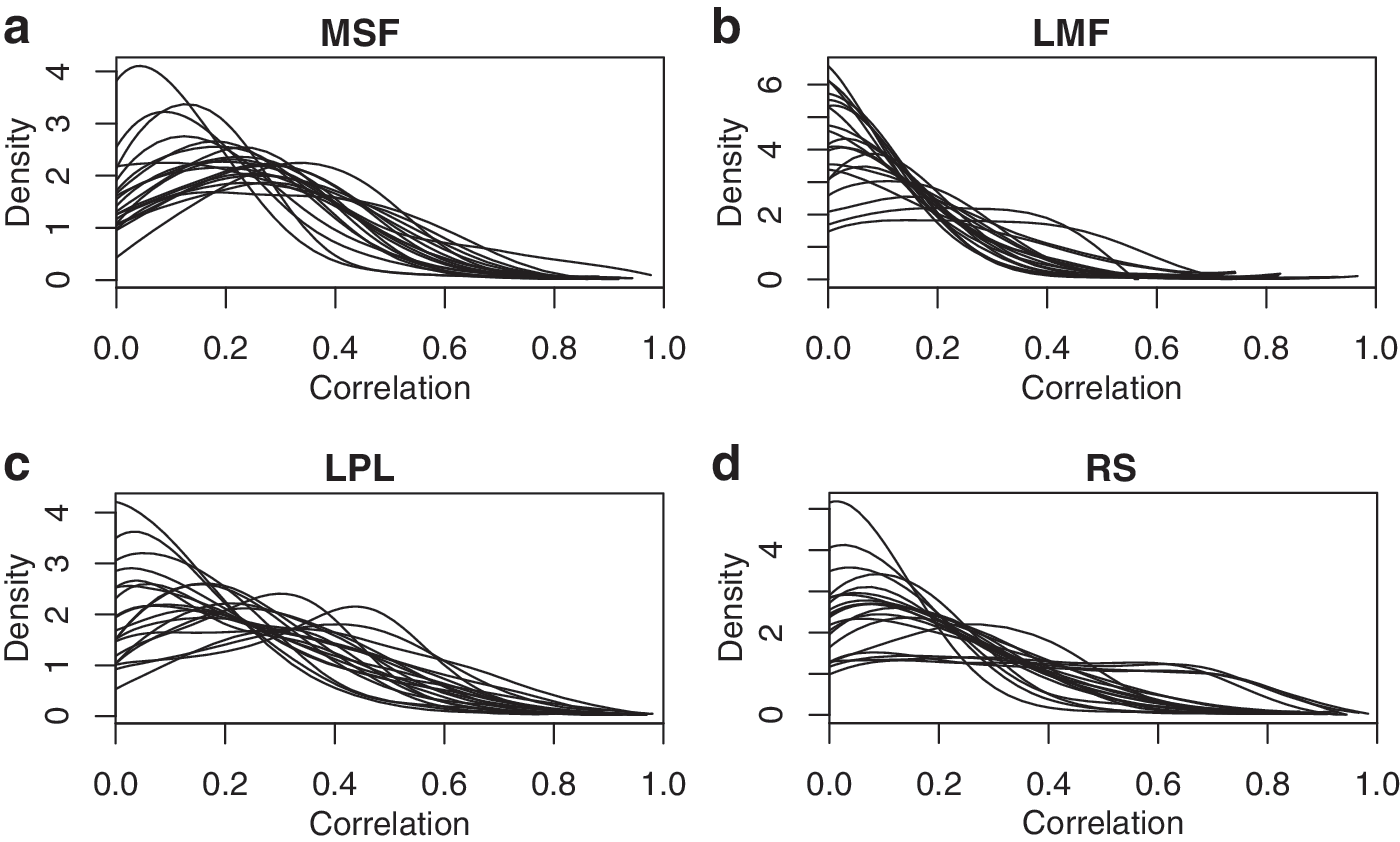
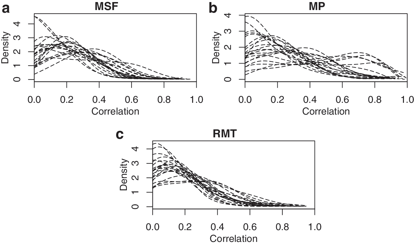
We begin by examining the subject-specific correlation densities for various regions. The intraregional connectivity densities for normal subjects are visualized in Figure 2 for the MSF, LMF, LPL, and RS regions and for Alzheimer's subjects in Figure 3 for the MSF, MP, and RMT regions. These regions were the most relevant predictors in the optimal models discovered in the regression analyses below; densities for the other regions showed similar patterns. To facilitate visualization, these densities are plotted for a randomly chosen subset of 20 subjects in each group. The local connectivity distributions fall into one of three classes: (1) unimodal with peak near 0, (2) unimodal with peak at moderate-to-high correlation values, and (3) flat over a wide range of correlations.
Local connectivity densities for 20 randomly chosen normal subjects for (a) MSF, (b) LMF, (c) LPL, and (d) RS regions. These regions correspond to the most relevant active predictors chosen in the regression analyses. LMF, left middle frontal; LPL, left parietal lobule; MSF, medial superior frontal; RS, right supramarginal.
Local connectivity densities for 20 randomly chosen Alzheimer's subjects for (a) MSF, (b) MP, and (c) RMT regions. These regions correspond to the most relevant active predictors chosen in the regression analyses. MP, medial prefrontal; RMT, right middle temporal.
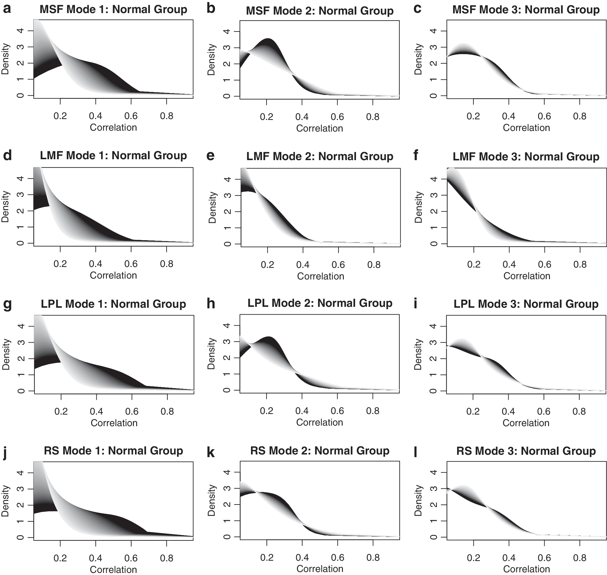
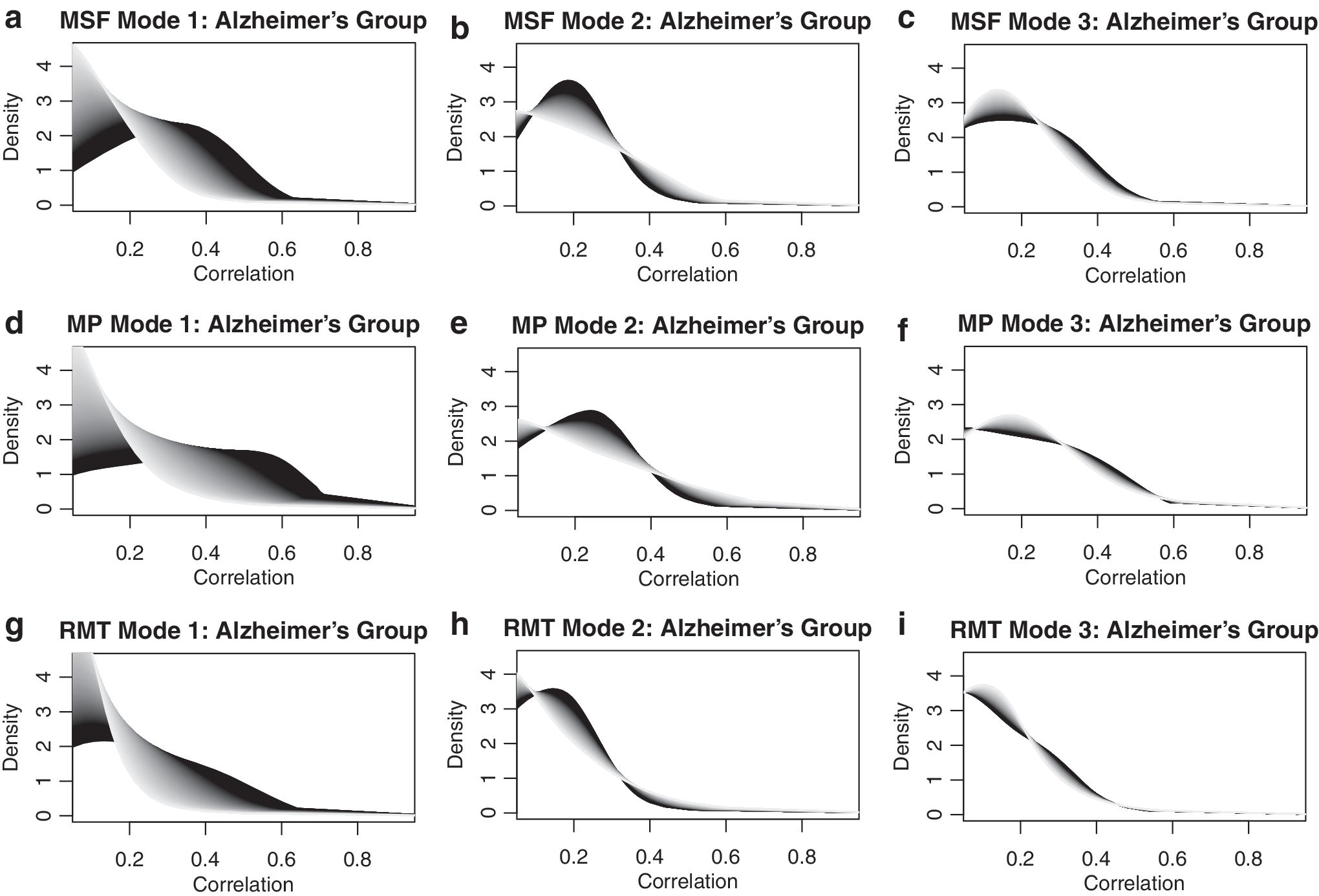
For both groups, application of the transformation methodology in Equation 3 followed by FPCA resulted in the selection of three FPC scores \documentclass{aastex}\usepackage{amsbsy}\usepackage{amsfonts}\usepackage{amssymb}\usepackage{bm}\usepackage{mathrsfs}\usepackage{pifont}\usepackage{stmaryrd}\usepackage{textcomp}\usepackage{portland, xspace}\usepackage{amsmath, amsxtra}\usepackage{upgreek}\pagestyle{empty}\DeclareMathSizes{10}{9}{7}{6}\begin{document}$$( { \xi _{ij1}} , { \xi _{ij2}} , { \xi _{ij3}} )$$ \end{document} to represent the densities \documentclass{aastex}\usepackage{amsbsy}\usepackage{amsfonts}\usepackage{amssymb}\usepackage{bm}\usepackage{mathrsfs}\usepackage{pifont}\usepackage{stmaryrd}\usepackage{textcomp}\usepackage{portland, xspace}\usepackage{amsmath, amsxtra}\usepackage{upgreek}\pagestyle{empty}\DeclareMathSizes{10}{9}{7}{6}\begin{document}$${f_{ij}}$$ \end{document}. The most common patterns of variability in these collections of density curves are represented by the transformation modes of variation in Equation 4, which are illustrated in Figures 4 and 5. It emerges that the first mode of variation embodies the shift from highly peaked connectivity densities near 0 (light gray extreme, high FPC score) to relatively flatter densities with substantial fractions of correlations >0.5 (black extreme, low FPC scores). The second mode of variation indicates the level of concentration of the distribution, that is, the extent to which the correlations concentrate near 0.25, while the third mode of variation quantifies concentration around 0.15. However, this last mode only accounts for a small fraction of the overall variability.
Mode of variation plots for the first three FPC scores of the MSF (a-c), LMF (d-f), LPL (g-i), and RS (j-l) regions in the cognitively normal group. Black (light gray) corresponds to low (high) values of the corresponding FPC scores, used as predictors in the regression models. For all regions, the first mode of variation indicates how much connectivity densities concentrate around 0, as well as how large it is around 0.6, while the second mode emphasizes the size of a mode around 0.25, and the third mode the size of a mode around 0.15. FPC, functional principal component.
Mode of variation plots for the first three FPC scores of the MSF (a-c), MP (d-f), and RMT (g-i) regions in the Alzheimer's group. Black (light gray) corresponds to low (high) values of the corresponding FPC score used in the regression models, where the interpretation of the three modes of variation is similar to that for the three modes of variation for the regions of the normal group.
Identifying connectivity–cognition associations
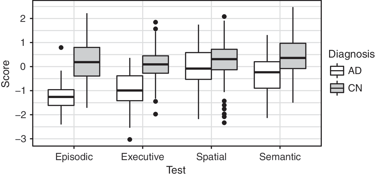
The response variables in our analysis are the following standardized measures of cognitive function: episodic memory, executive function, spatial memory, and semantic memory. Figure 6 shows the distribution of these values for the two samples of cognitively normal subjects and Alzheimer's subjects. As expected, scores are generally higher for normal subjects.
Box plots for the distributions of cognitive scores within each subject group. “AD” refers to the Alzheimer's disease group and “CN” to the cognitively normal group.
For the regression fits obtained from model (Equation 6), we report the sequentially selected regions for the different subject groups and each of the four cognitive scores in Table 1 for cognitively normal subjects and in Table 2 for Alzheimer's subjects. As some subjects had missing test scores, the total number of subjects used in each model is also indicated. Each group of included predictors was tested for significance using the postselection inferential technique described in Loftus and Taylor (2015), and p values <0.1 are shown in bold.
Postselection p Values for All Four Age-Corrected Cognitive Scores Using a Two-Step Stopping Criterion Based on Akaike Information Criterion for Cognitively Normal Subjects
Episodic
Executive
Spatial
Semantic
N = 152
N = 153
N = 139
N = 149
1
MSF (0.328)
LPL (0.830)
MSF (0.352)
LPL (0.394)
2
RMF (0.968)
LMF (0.071)
LMF (0.848)
LMF (0.089)
3
LPL (0.021)
LMT (0.706)
RPL (0.813)
—
4
LMT (0.373)
MSF (0.065)
RS (0.085)
—
5
RMT (0.549)
—
—
—
Rows indicate the order in which the regions are added to the model, with corresponding region-specific p values in parentheses. Each p value corresponds to the null hypothesis that the region can be removed from the model, assuming that previously added regions are included. p Values <0.1 are shown in bold.
LMF, left middle frontal; LMT, left middle temporal; LPL, left parietal lobule; MSF, medial superior frontal; RMF, right middle frontal; RMT, right middle temporal; RPL, right parietal lobule; RS, right supramarginal.
Postselection p Values for All Four Age-Corrected Cognitive Scores Using a Two-Step Stopping Criterion Based on Akaike Information Criterion for Alzheimer's Subjects
Episodic
Executive
Spatial
Semantic
N = 60
N = 61
N = 40
N = 59
1
MSF (0.073)
RPL (0.937)
PCP (0.215)
RMF (0.248)
2
MP (0.086)
MSF (0.205)
MP (0.278)
RMT (0.064)
3
—
—
RMF (0.973)
MSF (0.010)
4
—
—
—
LMF (0.795)
Rows indicate the order in which the regions are added to the model, with corresponding region-specific p values in parentheses. Each p value corresponds to the null hypothesis that the region can be removed from the model, assuming that previously added regions are included. p Values <0.1 are shown in bold.
To further elucidate the association of the connectivity densities with cognitive scores, we indicate in Tables 3 and 4 the direction of the association between each cognitive score and the first and second FPC scores for the regions with small p values in Tables 1 and 2. These are based on the sign of the coefficient estimate in the fitted model after forward selection.
Directional Associations Between the First Functional Principal Component Score and Cognitive Score
\documentclass{aastex}\usepackage{amsbsy}\usepackage{amsfonts}\usepackage{amssymb}\usepackage{bm}\usepackage{mathrsfs}\usepackage{pifont}\usepackage{stmaryrd}\usepackage{textcomp}\usepackage{portland, xspace}\usepackage{amsmath, amsxtra}\usepackage{upgreek}\pagestyle{empty}\DeclareMathSizes{10}{9}{7}{6}\begin{document}$$\uparrow$$ \end{document}, the higher the density peak near 0, the higher the test scores; \documentclass{aastex}\usepackage{amsbsy}\usepackage{amsfonts}\usepackage{amssymb}\usepackage{bm}\usepackage{mathrsfs}\usepackage{pifont}\usepackage{stmaryrd}\usepackage{textcomp}\usepackage{portland, xspace}\usepackage{amsmath, amsxtra}\usepackage{upgreek}\pagestyle{empty}\DeclareMathSizes{10}{9}{7}{6}\begin{document}$$\downarrow$$ \end{document}, the higher the density peak near 0, the lower the test scores.
Directional Associations Between the Second Functional Principal Component Score and Cognitive Score
\documentclass{aastex}\usepackage{amsbsy}\usepackage{amsfonts}\usepackage{amssymb}\usepackage{bm}\usepackage{mathrsfs}\usepackage{pifont}\usepackage{stmaryrd}\usepackage{textcomp}\usepackage{portland, xspace}\usepackage{amsmath, amsxtra}\usepackage{upgreek}\pagestyle{empty}\DeclareMathSizes{10}{9}{7}{6}\begin{document}$$\uparrow$$ \end{document}, the higher the peak near 0.25, the higher the test scores; \documentclass{aastex}\usepackage{amsbsy}\usepackage{amsfonts}\usepackage{amssymb}\usepackage{bm}\usepackage{mathrsfs}\usepackage{pifont}\usepackage{stmaryrd}\usepackage{textcomp}\usepackage{portland, xspace}\usepackage{amsmath, amsxtra}\usepackage{upgreek}\pagestyle{empty}\DeclareMathSizes{10}{9}{7}{6}\begin{document}$$\downarrow$$ \end{document}, the higher the density peak near 0.25, the lower the test scores.
For normal subjects, we find that densities with high peaks near 0 in the LPL region, that is, more concentrated lower connectivity levels, which are the densities indicated in light gray in Figure 4g–i, are associated with lower episodic performance, and the same pattern holds between MSF densities and executive scores, as well as RS densities and spatial scores. However, higher density peaks near 0 in the LMF region are found to be positively associated with both executive and semantic scores. For the Alzheimer's group, having lower density peaks near 0 in the MSF region is positively associated with both episodic and semantic memory, and the same relationship holds between the RMT connectivity and semantic scores. The reverse is true for the MP region and episodic score.
Regarding the second FPC scores in Table 4 for normal subjects, we find that episodic, executive, and spatial scores are negatively associated with densities that have distinctive modes around 0.25. That is, a high concentration of moderate local functional connectivity values is related to performance decline. This is reversed for semantic score, where higher semantic performance is associated with concentrated correlations around 0.25 in the LMF region for normal subjects and in the RMT and MSF regions for the Alzheimer's group.
Further visual interpretations of these findings are provided by contour plots based on the observed connectivity density/score pairs \documentclass{aastex}\usepackage{amsbsy}\usepackage{amsfonts}\usepackage{amssymb}\usepackage{bm}\usepackage{mathrsfs}\usepackage{pifont}\usepackage{stmaryrd}\usepackage{textcomp}\usepackage{portland, xspace}\usepackage{amsmath, amsxtra}\usepackage{upgreek}\pagestyle{empty}\DeclareMathSizes{10}{9}{7}{6}\begin{document}$$( {f_{ij}} , {Y_i} )$$ \end{document}. Here, the x and y axes correspond to the cognitive score and correlation level, respectively, and the value of the connectivity density is indicated by the color. These plots are shown in Figure 7 for three density/score combinations, two for the normal subjects and one for the Alzheimer's group. To more clearly discern the patterns in these plots, a smoothing step was applied along the cognitive score axis to reduce the noise in the data. The main relationship observed between LMF intraregional connectivity densities and executive score is that subjects with high executive performance tend to have higher density modes near 0, while for MSF connectivity densities, densities with modes near 0.2 are associated with higher executive scores. In the Alzheimer's group, higher density peaks at low connectivity values for intraregional connectivity densities in the RMT region are associated with lower semantic performance. These simple visual interpretations are confirmed by the numeric findings in Tables 3 and 4.
Smoothed contour plots of cognitive score/intraregional density relationships. (a) LMF region and executive score (normal group), (b) MSF region and executive score (normal group), and (c) RMT region and semantic score (Alzheimer's group).
Discussion and Conclusions
We introduce connectivity densities to quantify intraregional connectivity, using FDA methodology adapted to density functions and demonstrate that this quantification of intraregional connectivity can lead to specific findings that complement interregional connectivity studies and traditional interregional network analysis. As we demonstrate, the quantification of connectivity density functions can be complemented by group forward selection and accompanying postselection inference to discover relationships with other relevant covariates at the level of individual subjects.
In particular, our results demonstrate the value of utilizing entire distributions as predictors, where we use a nonlinear transformation method followed by FPCA to summarize each density in a vector of principal component scores. While these functional predictors contain a wealth of information, FPCA combined with the mode of variation plots simultaneously provides dimension reduction and interpretability. We conclude that intraregional connectivity contains valuable information to assess the brain function. Our methodology allows to efficiently quantify, visualize, and interpret key aspects of intraregional connectivity. Application of these novel methods revealed that intraregional connectivity is associated with cognitive scores in specific ways. These findings are validated by related previous findings in the literature.
Our observation of a positive association between lower intraregional connectivity with connectivity densities more concentrated around 0, and the executive function for the left middle frontal cortex is supported by previous studies. Lower activation of LMF has been found to be correlated with executive function (Kirova et al., 2015; Possin et al., 2014) and with better attention performance (Murphy et al., 2014). A negative correlation between gray matter volume in LMF and executive function has also been previously discussed (Breukelaar et al., 2017). Our methodology thus highlights the specific role played by intraregional connectivity in LMF.
It has also been previously observed that during episodic memory retrieval, several parietal regions are active, including inferior and superior parietal cortex (Hutchinson et al., 2015; Sajonz et al., 2010; Wagner et al., 2005) as well as the left inferior and superior parietal gyrus play a role (Hutchinson et al., 2015; Sajonz et al., 2010), suggesting that the activation of these regions is positively correlated with memory retrieval.
Frontal lobe deficit or dysfunction has been previously related to executive malfunction. Subjects with lesions on the frontal lobes, including in the MSF cortex, show lower executive function test performance (Roca et al., 2009). Especially subjects with damage in MSF regions are reported to perform particularly poor in tests related to speed response in the study of Stuss (2011), who hypothesized that the slower executive function is due to the failure of initiating or sustaining the activity in MSF. This hypothesis suggests a positive correlation between the executive function and activity in MSF.
Arnold et al. (2014) described a connection between spatial function scores and activity in the RS, right precentral cortex, and left hippocampus. Similarly, Bähner et al. (2015) reported that the magnitude of the interaction between bilateral, dorsolateral, right supramarginal cortex and hippocampus may predict spatial working memory performance.
Group analysis in the study of Wierenga et al. (2011) has shown that thinning of the RMT cortex in Alzheimer's disease patients is correlated with semantic test performance, where also the activation of the RMT cortex is reported when Alzheimer's disease subjects were performing certain semantic tasks. Finally, Seidenberg et al. (2009) observed that compared with a normal control group, subjects at high risk for Alzheimer's disease show greater activity in the RMT cortex.
While the emphasis of this article is a novel quantification of intraregional connectivity, the resulting analysis indicates that certain intraregional correlations are associated to some degree with the cognitive status of a subject. The direction of these associations varies across regions and also differs according to disease status.
Footnotes
Acknowledgment
This work was supported by the National Science Foundation grants DMS-1811888 and DMS-1712864.
Author Disclosure Statement
No competing financial interests exist.
References
1.
AchardS, SalvadorR, WhitcherB, SucklingJ, BullmoreE. 2006. A resilient, low-frequency, small-world human brain functional network with highly connected association cortical hubs. J Neurosci, 26:63–72.
BähnerF, DemanueleC, SchweigerJ, GerchenMF, ZamoscikV, UeltzhöfferK, et al.2015. Hippocampal–dorsolateral prefrontal coupling as a species-conserved cognitive mechanism: a human translational imaging study. Neuropsychopharmacology, 40:1674–1681.
BassettDS, NelsonBG, MuellerBA, CamchongJ, LimKO. 2012. Altered resting state complexity in schizophrenia. NeuroImage, 59:2196–2207.
6.
BetzelRF, ByrgeL, HeY, GoñiJ, ZuoX-N, SpornsO. 2014. Changes in structural and functional connectivity among resting-state networks across the human lifespan. NeuroImage, 102:345–357.
7.
BreukelaarIA, AnteesC, GrieveSM, FosterSL, GomesL, WilliamsLM, KorgaonkarMS. 2017. Cognitive control network anatomy correlates with neurocognitive behavior: a longitudinal study. Hum Brain Mapp, 38:631–643.
8.
BucknerRL, SepulcreJ, TalukdarT, KrienenFM, LiuH, HeddenT, et al.2009. Cortical hubs revealed by intrinsic functional connectivity: mapping, assessment of stability, and relation to Alzheimer's disease. J Neurosci, 29:1860–1873.
9.
CaiT, HallP. 2006. Prediction in functional linear regression. Ann Statistics, 34:2159–2179.
10.
ChenK, ZhangX, PetersenA, MüllerH-G. 2017. Quantifying infinitedimensional data: functional data analysis in action. Stat Biosci, 9:582–604.
FerreiraLK, BusattoGF. 2013. Resting-state functional connectivity in normal brain aging. Neurosci Biobehav Rev, 37:384–400.
13.
HallP, HorowitzJL. 2007. Methodology and convergence rates for functional linear regression. Ann Stat, 35:70–91.
14.
HanL, PengfeiZ, ZhaohuiL, FeiY, TingL, ChengD, ZhenchangW. 2015. Resting-state functional connectivity density mapping of etiology confirmed unilateral pulsatile tinnitus patients: altered functional hubs in the early stage of disease. Neuroscience, 310:27–37.
15.
HeJ, CarmichaelO, FletcherE, SinghB, IosifA-M, MartinezO, et al.2012. Influence of functional connectivity and structural MRI measures on episodic memory. Neurobiol Aging, 33:2612–2620.
16.
HintonL, CarterK, ReedBR, BeckettL, LaraE, DeCarliC, MungasD. 2010. Recruitment of a community-based cohort for research on diversity and risk of dementia. Alzheimer Dis Assoc Disord, 24:234.
17.
HosseiniS, HoeftF, KeslerSR. 2012. GAT: a graph-theoretical analysis toolbox for analyzing between-group differences in large-scale structural and functional brain networks. PLoS One, 7:e40709.
18.
HutchinsonJB, UncapherMR, WagnerAD. 2015. Increased functional connectivity between dorsal posterior parietal and ventral occipitotemporal cortex during uncertain memory decisions. Neurobiol Learn Memory, 117:71–83.
19.
JonesMC, RiceJA. 1992. Displaying the important features of large collections of similar curves. Am Stat, 46:140–145.
20.
KirovaA-M, BaysRB, LagalwarS. 2015. Working memory and executive function decline across normal aging, mild cognitive impairment, and Alzheimer's disease. Biomed Res Int, 2015:748212.
21.
KneipA, UtikalKJ. 2001. Inference for density families using functional principal component analysis. J Am Stat Assoc, 96:519–542.
22.
LoftusJR, TaylorJE. 2015. Selective inference in regression models with groups of variables, arXiv Preprint arXiv:1511.01478.
23.
Lopez-LarsonMP, AndersonJS, FergusonMA, Yurgelun-ToddD. 2011. Local brain connectivity and associations with gender and age. Dev Cogn Neurosc, 1:187–197.
24.
MurphyCM, ChristakouA, DalyEM, EckerC, GiampietroV, BrammerM, et al.2014. Abnormal functional activation and maturation of fronto-striato-temporal and cerebellar regions during sustained attention in autism spectrum disorder. Am J Psychiatry, 171:1107–1116.
25.
ParzenE. 1962. On estimation of a probability density function and mode. Ann Math Stat, 33:1065–1076.
26.
PetersenA, MüllerH-G. 2016. Functional data analysis for density functions by transformation to a Hilbert space. Ann Stat, 44:183–218.
27.
PossinKL, LaMarreAK, WoodKA, MungasDM, KramerJH. 2014. Ecological validity and neuroanatomical correlates of the NIH EXAMINER executive composite score. J Int Neuropsychol Soc, 20:20–28.
28.
QiR, ZhangLJ, ChenHJ, ZhongJ, LuoS, KeJ, et al.2015. Role of local and distant functional connectivity density in the development of minimal hepatic encephalopathy. Sci Rep, 5:13720.
29.
RamsayJO, SilvermanBW. 2005. Functional Data Analysis, Springer Series in Statistics, 2nd ed. New York: Springer.
30.
RocaM, ParrA, ThompsonR, WoolgarA, TorralvaT, AntounN, et al.2009. Executive function and fluid intelligence after frontal lobe lesions. Brain, 133:234–247.
31.
RosenblattM. 1956. Remarks on some nonparametric estimates of a density function. Ann Math Stat. 27:832–837.
32.
SajonzB, KahntT, MarguliesDS, ParkSQ, WittmannA, StoyM, et al.2010. Delineating self-referential processing from episodic memory retrieval: common and dissociable networks. NeuroImage, 50:1606–1617.
33.
SeidenbergM, GuidottiL, NielsonKA, WoodardJL, DurgerianS, AntuonoP, et al.2009. Semantic memory activation in individuals at risk for developing Alzheimer disease. Neurology, 73:612–620.
34.
ShuklaDK, KeehnB, MüllerRA. 2010. Regional homogeneity of fMRI time series in autism spectrum disorders. Neurosci Lett, 476:46–51.
35.
SilvermanBW. 1986. Density Estimation for Statistics and Data Analysis, Monographs on Statistics and Applied Probability. London: Chapman and Hall Ltd.
36.
StussDT. 2011. Functions of the frontal lobes: relation to executive functions. J Int Neuropsychol Soc, 17:759–765.
37.
TomasiD, VolkowND. 2010. Functional connectivity density mapping. Proc Natl Acad Sci USA, 107:9885–9890.
38.
TomasiD, VolkowND. 2011. Association between functional connectivity hubs and brain networks. Cerebral Cortex, 21:2003–2013.
WandMP, JonesMC. 1995. Kernel Smoothing, Vol. 60 of Monographs on Statistics and Applied Probability. London: Chapman and Hall Ltd.
43.
WangJ-L, ChiouJ-M, MüllerH-G. 2016. Functional data analysis. Annu Rev Stat Appl, 3:257–295.
44.
WierengaCE, StrickerNH, McCauleyA, SimmonsA, JakAJ, ChangY-L, et al.2011. Altered brain response for semantic knowledge in Alzheimer's disease. Neuropsychologia, 49:392–404.
45.
WorsleyKJ, ChenJ-I, LerchJ, EvansAC. 2005. Comparing functional connectivity via thresholding correlations and singular value decomposition. Philos Trans R Soc B Biol Sci, 360:913–920.
46.
WuT, LongX, ZangY, WangL, HallettM, LiK, ChanP. 2009. Regional homogeneity changes in patients with Parkinson's disease. Hum Brain Mapp, 30:1502–1510.
47.
ZaleskyA, FornitoA, BullmoreE. 2012. On the use of correlation as a measure of network connectivity. NeuroImage, 60:2096–2106.
48.
ZangY, JiangT, LuY, HeY, TianL. 2004. Regional homogeneity approach to fMRI data analysis. Neuroimage, 22:394–400.