Individual Activation Patterns After the Stimulation of Different Motor Areas: A Transcranial Magnetic Stimulation

Abstract

The combination of transcranial magnetic stimulation (TMS) and electroencephalography (EEG) enables one to study effective connectivity and activation order in neuronal networks. To characterize effective connectivity originating from the primary motor cortex (M1), dorsal premotor area (PMd), and supplementary motor area (SMA). Three right-handed volunteers (two men, aged 25–30 years) participated in a navigated TMS–EEG experiment. M1, PMd, and SMA over the nondominant hemisphere were stimulated with 150 TMS pulses. Minimum-norm estimates were derived from the EEG data to estimate the spatial spreading of TMS-elicited neuronal activation on an individual level. The activation order of the cortical areas varied depending on the stimulated area. There were similarities and differences in the spatial distribution of the TMS-evoked potentials between subjects. Similarities in cortical activation patterns were seen at short poststimulus latencies and the differences at long latencies. This pilot study suggests that cortical activation patterns and the activation order of motor areas differ interindividually and depend on the stimulated motor area. It further indicates that TMS-activated effective connections or underlying structural connections vary between subjects. The spatial patterns of TMS-evoked potentials differ between subjects especially at long latencies, when probably more complex neuronal networks are active.

Introduction

Transcranial magnetic stimulation (TMS) is a noninvasive method for exciting cortical neurons directly below the stimulation coil and indirectly elsewhere in the cortex, in subcortical gray matter, and in the spinal cord through cortical, subcortical, and corticospinal connections (Barker et al., 1985; Di Lazzaro and Ziemann, 2013; Di Lazzaro et al., 1998, 2017; Nakamura et al., 1996). TMS can be used to study the function of the primary motor cortex (M1), which controls muscle movements in the body through the pyramidal tracts (Barker et al., 1985). The elicited reactions can be quantified by measuring motor-evoked potentials (MEPs) with electromyography (EMG) (Hallett, 2000). The observed MEPs depend on excitatory and inhibitory mechanisms at different neuronal levels along the motor pathway from M1 to the muscle (Ferreri et al., 2003; Rossini and Rossi, 2007). The combination of TMS and EMG can also inform about the function of cortico-cortical connections between M1 and other cortical areas as well as inter- and intracortical inhibitory and facilitatory mechanisms in M1 (Arai and Yoshikazu, 2012; Bortoletto et al., 2015; Cona and Semenza, 2017; Ferbert et al., 1992; Kujirai et al., 1993).

M1 is assisted by nonprimary motor areas and the cerebellum in the selection and execution of correct movement sequences (Ferreri et al., 2011; Guye et al., 2003; Johansen-Berg et al., 2004; Li et al., 2015; Orgogozo and Larsen, 1979; Picard and Strick, 2001). Nonprimary motor areas—the dorsal premotor area (PMd) and the supplementary motor area (SMA)—are located anterior to M1 in the frontal lobe, and are strongly connected to M1 and other cortical areas in anatomy (Geyer, 2004; Penfield and Welch, 1951). The spreading of cortical activation through neuronal connections from the motor cortex to other areas can be observed by electroencephalography (EEG) measured concurrently with TMS (TMS–EEG) (Komssi and Kähkönen, 2006; Lee et al., 2003).

TMS-evoked potentials (TEPs) in scalp EEG signals can be monitored from a few milliseconds after the stimulus until about 300 ms poststimulus (Komssi and Kähkönen, 2006). The first responses to TMS are typically short lasting, whereas the duration of later deflections is usually longer (Ilmoniemi and Karhu, 2012). Typical latencies and scalp distributions after M1 (Bonato et al., 2006; Ferreri et al., 2011; Ilmoniemi et al., 1997; Lioumis et al., 2009), prefrontal (Kähkönen et al., 2005; Lioumis et al., 2009), and sensorimotor-cortex stimulation (Komssi et al., 2002) have been described. TEPs reflect the spreading of activation between cortical areas through intra- and intercortical connections (Guye et al., 2003; Kandel and Schwartz, 1985).

In this study, we aimed to determine resting-state effective connectivity originating from the nondominant M1 and nonprimary motor areas in healthy subjects using TMS–EEG. We compared cortical activation patterns between stimulation sites and subjects.

Materials and Methods

Subjects

Three right-handed volunteers (S1, S2, and S3) were studied (mean age 27, range 25–30 years; two men). The participants were informed of the research procedures, and they gave their written informed consent before the experiment. The study was approved by the Ethics Committee of Helsinki University Hospital; it was compliant with the Declaration of Helsinki.

EEG, EMG, and TMS

Before the experiment, magnetic resonance images (MRIs) of the head were obtained from each subject to enable the use of a navigated brain stimulation (NBS; Nexstim Plc, Helsinki, Finland) system and to make a volume-conduction model needed in the analysis. A 60-channel EEG cap with the TMS-compatible Nexstim eXimia EEG device was used to record TEPs. The electrode contacts were prepared so that the impedances were <5 kΩ or are as low as possible if 5 kΩ could not be reached. The reference electrode was attached to the forehead and the ground electrode to the right cheekbone. Electrooculography electrodes were placed on the left side of the left eye and just above the right eyebrow. The nasion, the preauricular points, and eight points along the head were registered with a 3D-digitizing pen before the stimulation to allow the NBS system to track the location of the stimulation coil with respect to the head. MEPs were recorded from the left abductor pollicis brevis (APB) muscle using the Nexstim EMG system.

After fixing the EEG cap, sequences of biphasic TMS pulses were delivered with Nexstim's transcranial magnetic stimulator and figure-of-eight coil (outer loop diameter 70 mm). The stimuli were targeted to the right hemisphere using the NBS system; the subjects sat relaxed on a chair and were instructed to keep their eyes open.

The EEG signals were recorded with a bandwidth of 0.1–350 Hz and sampled at the rate of 1450 Hz. A sample-and-hold circuit prevented the TMS-induced artifact from saturating the amplifier during the pulse (Virtanen et al., 1999). To avoid the appearance of auditory-evoked potentials, the sound of the TMS coil was masked by playing white noise at a safe noise level through headphones to the subject's ears (Nikouline et al., 1999). The locations of the EEG electrodes and the reference electrode were digitized using the NBS system. The electrode coordinates were later used in constructing the subject-specific volume-conduction models that were needed in the source estimation.

Stimulation sites

The optimal representation area in the right M1 of the left-hand APB was determined by stimulating the precentral gyrus along the central sulcus, keeping the TMS-induced electric field (E-field) optimally oriented perpendicular to the sulcal wall (Fox et al., 2004; Thielscher et al., 2011). The mapping of the representation area was done with a stimulation intensity (SI) that produced an E-field of ∼80–100 V/m at the navigation depth of 21 mm; the exact value of SI was tuned for each subject so that MEP amplitudes of ∼0.5–1 mV were elicited. The stimulation target producing the largest and most reproducible MEPs in the APB was chosen as the optimal representation area.

The stimulation sites in PMd and SMA were chosen based on individual brain anatomy. The caudal part of the middle frontal gyrus anterior to the precentral gyrus and inferior to the superior frontal gyrus was selected for the stimulation site of PMd (Geyer, 2004; Penfield and Jasper, 1954; Penfield and Welch, 1951); the stimuli were targeted to the sulcus between the superior and middle frontal gyri so that the direction of the peak E-field was toward the middle frontal gyrus. The caudal part of the superior frontal gyrus next to the interhemispheric fissure was selected for the stimulation site of SMA (Johansen-Berg et al., 2004; Penfield and Welch, 1951); the stimuli were targeted perpendicularly to the interhemispheric fissure, with the strongest E-field oriented toward the superior frontal gyrus. The targets and the corresponding E-field directions for subject S3 are shown in Figure 1.

FIG. 1.

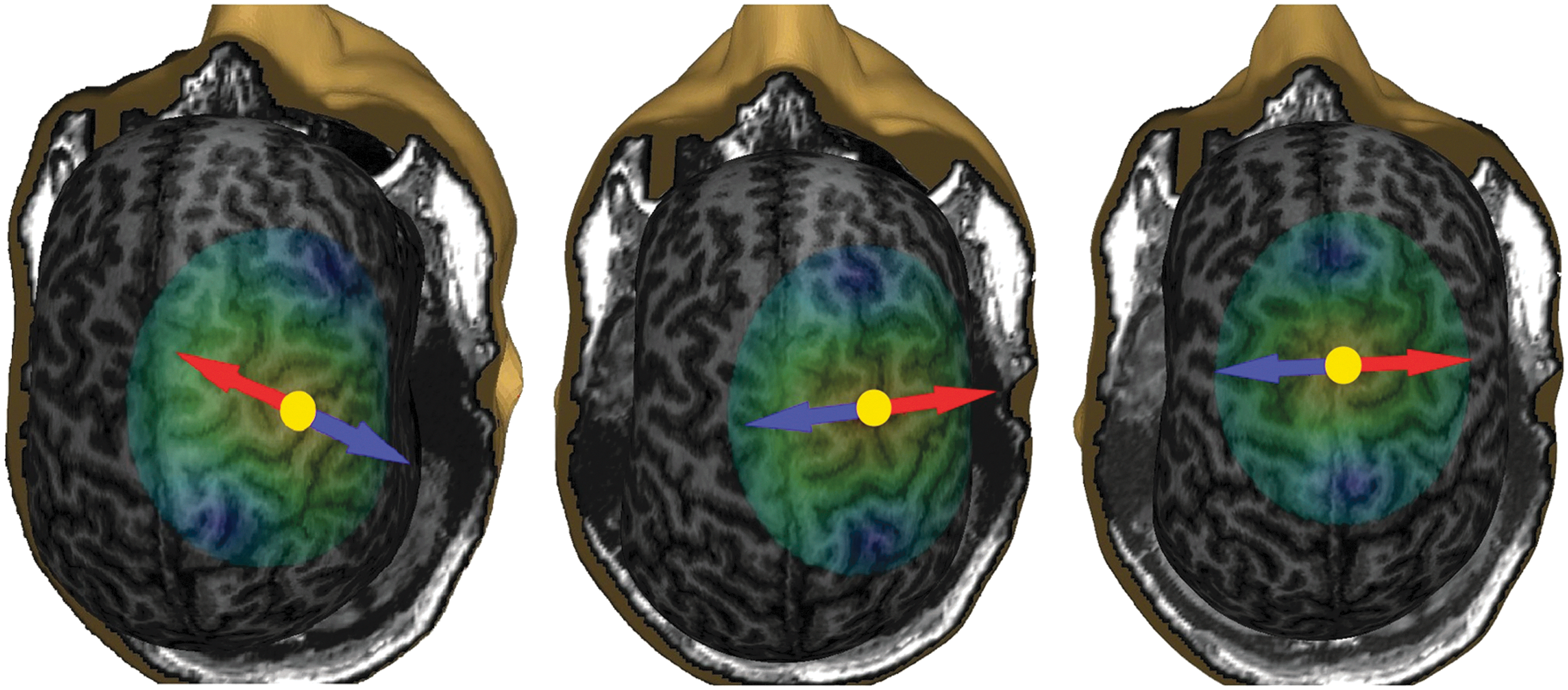
Stimulation targets of S4: left, M1; middle, PMd; right, SMA. The yellow dots between the blue and red arrows indicate the locations of the E-field maxima and the arrows indicate the directions of the peak E-fields. The stimulation was aimed at the direction of the red arrow. E-field, electric field; M1, primary motor cortex; PMd, dorsal premotor area; SMA, supplementary motor area.

Stimulation parameters

The motor threshold (MT) was defined from the optimal target in M1 as the smallest SI producing at least 5 out of 10 MEPs with a peak-to-peak amplitude higher than 50 μV measured from the left APB. After the MT determination, each subject received 150 stimuli (randomized interstimulus interval [ISI] of 3.0–3.5 sec) to each of the 3 stimulation sites (450 pulses in total) with an SI that produced 90% of the E-field of the MT determined at the navigation depth of 21 mm. A subthreshold SI was chosen to minimize EEG contamination from muscle artifacts (Mutanen et al., 2013) and any MEP-related somatosensory responses. In contrast, the SI was chosen to be near the MT value as suggested by Kähkönen et al. (2004) when prefrontal areas are stimulated. Fiori et al. (2017) showed that SI of 90% of MT was sufficient to demonstrate interhemispheric connectivity.

Computation of the lead fields

Using FreeSurfer software (Fischl et al., 2002) and individual T1-weighted MRIs, the boundary of white and gray matter was segmented and meshed. The boundaries of skull and scalp were segmented with BrainSuite (Shattuck and Leahy, 2002). Next, the segmentations were visually checked to match with the MRI, and the coordinates of the EEG electrodes were coregistered with the 3D reconstruction of the segmented MRI using MATLAB (The Mathworks, Inc., Natick, MA).

To take into account the effects of the conductivity profile of the head, we modeled the head as a three-compartment conductor consisting of the intracranial volume, skull, and scalp, with conductivities of 0.33, 0.0132, and 0.33 S/m, respectively. The model was solved with the boundary element method that was formulated using the isolated source approach (Stenroos and Sarvas, 2012).

The EEG signal is understood to originate mainly from postsynaptic activity of pyramidal neurons, which is in macroscopic scale modeled in terms of primary current density \documentclass{aastex}\usepackage{amsbsy}\usepackage{amsfonts}\usepackage{amssymb}\usepackage{bm}\usepackage{mathrsfs}\usepackage{pifont}\usepackage{stmaryrd}\usepackage{textcomp}\usepackage{portland, xspace}\usepackage{amsmath, amsxtra}\usepackage{upgreek}\pagestyle{empty}\DeclareMathSizes{10}{9}{7}{6}\begin{document}$${ {\overline {\rm J}} ^{\rm P}} \left( { \bf{r}} \right)$$ \end{document} . We modeled the primary current density as a linear combination of current dipoles that were lying evenly on the cortical boundary and oriented perpendicular to that boundary according to the dominating orientation of pyramidal dendrites. The dipoles were placed onto the vertices of the downsampled cortical mesh (5124 vertices); the scalp topography due to each unit-strength dipole was computed resulting in a lead-field matrix \documentclass{aastex}\usepackage{amsbsy}\usepackage{amsfonts}\usepackage{amssymb}\usepackage{bm}\usepackage{mathrsfs}\usepackage{pifont}\usepackage{stmaryrd}\usepackage{textcomp}\usepackage{portland, xspace}\usepackage{amsmath, amsxtra}\usepackage{upgreek}\pagestyle{empty}\DeclareMathSizes{10}{9}{7}{6}\begin{document}$${ \bf{L}}$$ \end{document} with dimensions of 60 × 5124. Each column of \documentclass{aastex}\usepackage{amsbsy}\usepackage{amsfonts}\usepackage{amssymb}\usepackage{bm}\usepackage{mathrsfs}\usepackage{pifont}\usepackage{stmaryrd}\usepackage{textcomp}\usepackage{portland, xspace}\usepackage{amsmath, amsxtra}\usepackage{upgreek}\pagestyle{empty}\DeclareMathSizes{10}{9}{7}{6}\begin{document}$${ \bf{L}}$$ \end{document} describes the signal topography of one focal “source,” whereas each row represents the sensitivity of each EEG sensor to activity across the brain.

Data processing

The EEG data were analyzed offline with MATLAB. At first, the data over trials were averaged from −300 to 500 ms with respect to the transcranial magnetic stimulus. Then the EEG signal and \documentclass{aastex}\usepackage{amsbsy}\usepackage{amsfonts}\usepackage{amssymb}\usepackage{bm}\usepackage{mathrsfs}\usepackage{pifont}\usepackage{stmaryrd}\usepackage{textcomp}\usepackage{portland, xspace}\usepackage{amsmath, amsxtra}\usepackage{upgreek}\pagestyle{empty}\DeclareMathSizes{10}{9}{7}{6}\begin{document}$${ \bf{L}}$$ \end{document} were average referenced. Next, the source-estimate-utilizing noise-discarding (SOUND) algorithm (Mutanen et al., 2018) was applied to the data to identify and suppress sensor noise or artifacts. The SOUND algorithm evaluates the reliability of the signal in each channel by comparing this signal with that obtained from a source estimate derived from the signals in all the other channels. Once the noise levels in all channels are known, cleaned signals can be obtained from them by constructing optimal linear combinations as in Wiener filtering.

After SOUND algorithm, signal-space projection (SSP) combined with source-informed reconstruction (SIR) (Mutanen et al., 2016) was used to delete muscle artifacts (two to nine artifact components were removed from each data set). The number of the extracted artifact components was determined as explained in Mutanen et al. (2016). SSP was used to suppress the effect of the artifacts by estimating artifact and brain subspaces. A linear operator was constructed using these subspaces to find an estimate of the sources. Then SIR was used to reconstruct the evoked brain activity in the original signal space using the original lead-field matrix and the obtained source estimate (Mutanen et al., 2016). After these steps, the data were bandpass filtered at 2–80 Hz using a second-order Butterworth filter with zero padding. The analysis of evoked EEG responses was done separately for all trials, odd trials, and even trials to verify the repeatability of the results.

Signal analysis

The preprocessed EEG data were used to calculate the global mean field amplitude (GMFA) as \documentclass{aastex}\usepackage{amsbsy}\usepackage{amsfonts}\usepackage{amssymb}\usepackage{bm}\usepackage{mathrsfs}\usepackage{pifont}\usepackage{stmaryrd}\usepackage{textcomp}\usepackage{portland, xspace}\usepackage{amsmath, amsxtra}\usepackage{upgreek}\pagestyle{empty}\DeclareMathSizes{10}{9}{7}{6}\begin{document} \begin{align*}{ \rm { GMFA } } \left( t \right) = \sqrt { \frac { { \mathop \sum \nolimits_ { i = 1 } ^N { { \left( { { V_i } \left( t \right) - { V_ { { \rm { mean } } } } \left( t \right) } \right) } ^2 } } } { N } } , \tag { 1 } \end{align*} \end{document}

where t is the time, V_i is the potential at electrode i, and V _mean is the average potential of the N electrodes (Lehmann and Skrandies, 1980).

The TMS-evoked activity at time t was considered significant if the GMFA at that time was >95% of the GMFA values measured during the baseline (−300 to 0 ms), as earlier described by Massimini et al. (2005). An example of significant activity is shown in Figure 2. From the significant activity, the poststimulus peaks with typical TEP latencies (near 18, 30, 44, 50, 100, and 180 ms) were visually identified, and signal topographies in these time instants were used for source analysis (Hämäläinen and Ilmoniemi, 1994; Lehmann and Skrandies, 1980; Lioumis et al., 2009).

FIG. 2.

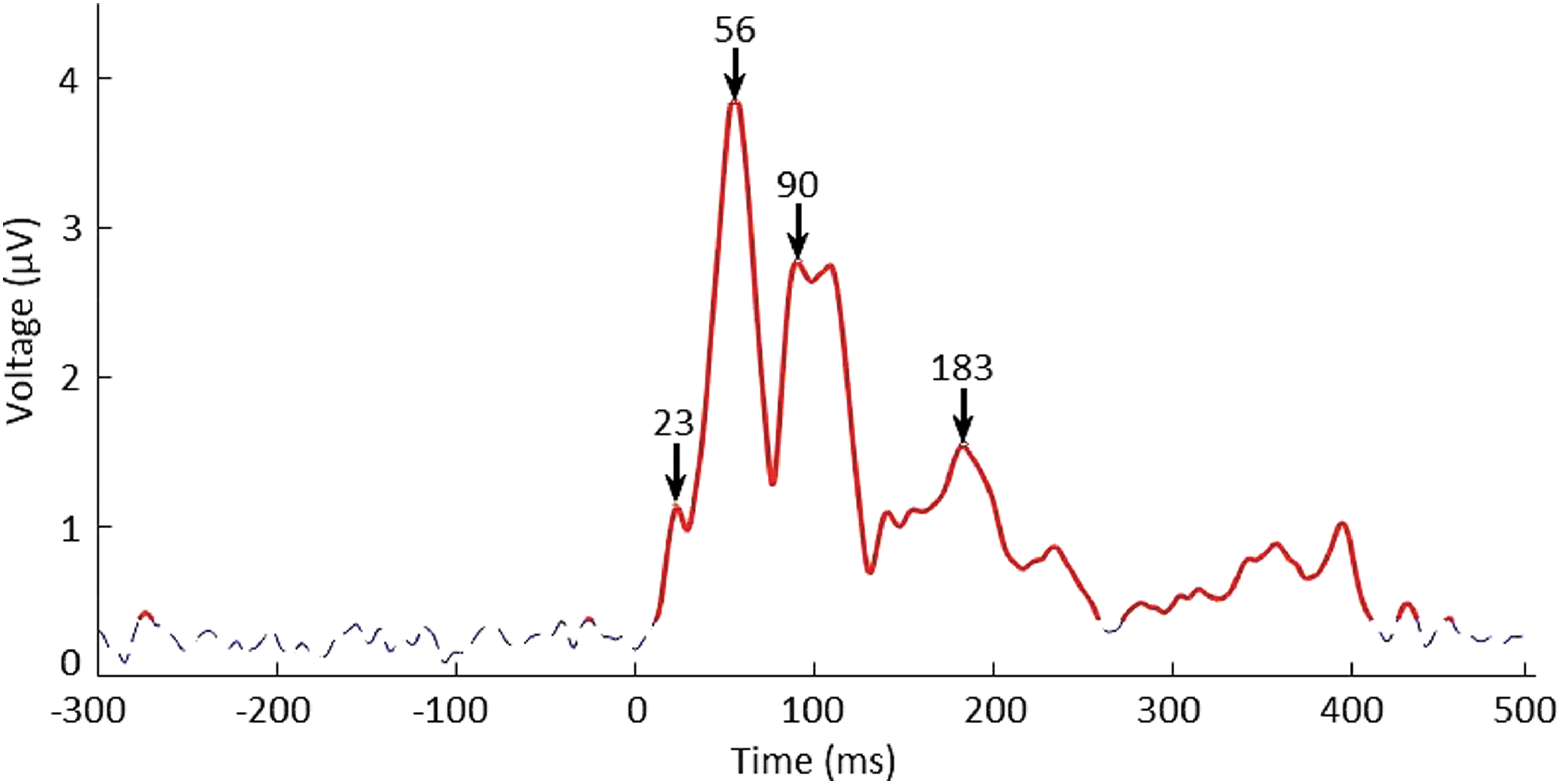
GMFA of S1 for the right M1 stimulation. The blue dotted line represents the noise that defines our threshold level (95% of the baseline activity), and the solid red line represents the brain signal (above the 95th percentile of the baseline values). Zero indicates the time of stimulus delivery. In this case, there are four dominant peaks: at 23, 56, 90, and 183 ms. GMFA, global mean field amplitude.

Minimum-norm estimation

Source analysis was carried out using linear distributed source estimation: the measured data are assumed to follow the linear measurement model: \documentclass{aastex}\usepackage{amsbsy}\usepackage{amsfonts}\usepackage{amssymb}\usepackage{bm}\usepackage{mathrsfs}\usepackage{pifont}\usepackage{stmaryrd}\usepackage{textcomp}\usepackage{portland, xspace}\usepackage{amsmath, amsxtra}\usepackage{upgreek}\pagestyle{empty}\DeclareMathSizes{10}{9}{7}{6}\begin{document} \begin{align*}{ \bf{m}} = { \bf{Ls}} + { \bf{n}} , \tag{2} \end{align*} \end{document}

where \documentclass{aastex}\usepackage{amsbsy}\usepackage{amsfonts}\usepackage{amssymb}\usepackage{bm}\usepackage{mathrsfs}\usepackage{pifont}\usepackage{stmaryrd}\usepackage{textcomp}\usepackage{portland, xspace}\usepackage{amsmath, amsxtra}\usepackage{upgreek}\pagestyle{empty}\DeclareMathSizes{10}{9}{7}{6}\begin{document}$${ \bf{m}}$$ \end{document} is the measurement from one time instant, \documentclass{aastex}\usepackage{amsbsy}\usepackage{amsfonts}\usepackage{amssymb}\usepackage{bm}\usepackage{mathrsfs}\usepackage{pifont}\usepackage{stmaryrd}\usepackage{textcomp}\usepackage{portland, xspace}\usepackage{amsmath, amsxtra}\usepackage{upgreek}\pagestyle{empty}\DeclareMathSizes{10}{9}{7}{6}\begin{document}$${ \bf{L}}$$ \end{document} is the lead-field matrix, \documentclass{aastex}\usepackage{amsbsy}\usepackage{amsfonts}\usepackage{amssymb}\usepackage{bm}\usepackage{mathrsfs}\usepackage{pifont}\usepackage{stmaryrd}\usepackage{textcomp}\usepackage{portland, xspace}\usepackage{amsmath, amsxtra}\usepackage{upgreek}\pagestyle{empty}\DeclareMathSizes{10}{9}{7}{6}\begin{document}$${ \bf{s}}$$ \end{document} is the source distribution (the amplitudes of the cortical dipoles), and \documentclass{aastex}\usepackage{amsbsy}\usepackage{amsfonts}\usepackage{amssymb}\usepackage{bm}\usepackage{mathrsfs}\usepackage{pifont}\usepackage{stmaryrd}\usepackage{textcomp}\usepackage{portland, xspace}\usepackage{amsmath, amsxtra}\usepackage{upgreek}\pagestyle{empty}\DeclareMathSizes{10}{9}{7}{6}\begin{document}$${ \bf{n}}$$ \end{document} is noise. As the inverse problem of solving \documentclass{aastex}\usepackage{amsbsy}\usepackage{amsfonts}\usepackage{amssymb}\usepackage{bm}\usepackage{mathrsfs}\usepackage{pifont}\usepackage{stmaryrd}\usepackage{textcomp}\usepackage{portland, xspace}\usepackage{amsmath, amsxtra}\usepackage{upgreek}\pagestyle{empty}\DeclareMathSizes{10}{9}{7}{6}\begin{document}$${ \bf{s}}$$ \end{document} from Equation (2) is ill-posed, we used regularized minimum-norm estimate (MNE) to estimate \documentclass{aastex}\usepackage{amsbsy}\usepackage{amsfonts}\usepackage{amssymb}\usepackage{bm}\usepackage{mathrsfs}\usepackage{pifont}\usepackage{stmaryrd}\usepackage{textcomp}\usepackage{portland, xspace}\usepackage{amsmath, amsxtra}\usepackage{upgreek}\pagestyle{empty}\DeclareMathSizes{10}{9}{7}{6}\begin{document}$${ \bf{s}}$$ \end{document} (Hämäläinen and Ilmoniemi, 1994; Matsuura and Okabe, 1995; Sarvas, 1987): we chose the solution that reconstructs the relevant part of \documentclass{aastex}\usepackage{amsbsy}\usepackage{amsfonts}\usepackage{amssymb}\usepackage{bm}\usepackage{mathrsfs}\usepackage{pifont}\usepackage{stmaryrd}\usepackage{textcomp}\usepackage{portland, xspace}\usepackage{amsmath, amsxtra}\usepackage{upgreek}\pagestyle{empty}\DeclareMathSizes{10}{9}{7}{6}\begin{document}$${ \bf{m}}$$ \end{document} with minimum L ² norm of \documentclass{aastex}\usepackage{amsbsy}\usepackage{amsfonts}\usepackage{amssymb}\usepackage{bm}\usepackage{mathrsfs}\usepackage{pifont}\usepackage{stmaryrd}\usepackage{textcomp}\usepackage{portland, xspace}\usepackage{amsmath, amsxtra}\usepackage{upgreek}\pagestyle{empty}\DeclareMathSizes{10}{9}{7}{6}\begin{document}$${ \bf{s}}$$ \end{document} . The solution is of the form \documentclass{aastex}\usepackage{amsbsy}\usepackage{amsfonts}\usepackage{amssymb}\usepackage{bm}\usepackage{mathrsfs}\usepackage{pifont}\usepackage{stmaryrd}\usepackage{textcomp}\usepackage{portland, xspace}\usepackage{amsmath, amsxtra}\usepackage{upgreek}\pagestyle{empty}\DeclareMathSizes{10}{9}{7}{6}\begin{document} \begin{align*} \widehat { \bf{s}} = {{ \bf{L}}^{ \bf{T}}}{ ( { \bf{L}}{{ \bf{L}}^{ \bf{T}}} + {{ \rm{ \lambda }}^2}{{ \bf{C}}_{{ \bf{n}} \;}} ) ^{ - 1}}{ \bf{m}} , \tag{3} \end{align*} \end{document}

The regularization parameter \documentclass{aastex}\usepackage{amsbsy}\usepackage{amsfonts}\usepackage{amssymb}\usepackage{bm}\usepackage{mathrsfs}\usepackage{pifont}\usepackage{stmaryrd}\usepackage{textcomp}\usepackage{portland, xspace}\usepackage{amsmath, amsxtra}\usepackage{upgreek}\pagestyle{empty}\DeclareMathSizes{10}{9}{7}{6}\begin{document}$${{{\lambda }}^2}$$ \end{document} was calculated as suggested in Lin et al. (2006): \documentclass{aastex}\usepackage{amsbsy}\usepackage{amsfonts}\usepackage{amssymb}\usepackage{bm}\usepackage{mathrsfs}\usepackage{pifont}\usepackage{stmaryrd}\usepackage{textcomp}\usepackage{portland, xspace}\usepackage{amsmath, amsxtra}\usepackage{upgreek}\pagestyle{empty}\DeclareMathSizes{10}{9}{7}{6}\begin{document} \begin{align*}{ { \rm { \lambda } } ^2 } = { \frac { { \rm { trace } } \left( { { { \bf { L } } _ { \bf { w } } } { { \bf { L } } _ { \bf { w } } } ^\textbf { \textit { T } } } \right) } { \left( { N { \rm { \;SNR } } } \right) } } , \tag { 4 } \end{align*} \end{document}

where S_j is the poststimulus signal and n_j is the noise in sensor j (Raz et al., 1988). The signal topography plots of \documentclass{aastex}\usepackage{amsbsy}\usepackage{amsfonts}\usepackage{amssymb}\usepackage{bm}\usepackage{mathrsfs}\usepackage{pifont}\usepackage{stmaryrd}\usepackage{textcomp}\usepackage{portland, xspace}\usepackage{amsmath, amsxtra}\usepackage{upgreek}\pagestyle{empty}\DeclareMathSizes{10}{9}{7}{6}\begin{document}$${ \bf{m}}$$ \end{document} were drawn using EEGLAB (Delorme and Makeig, 2004), and the source estimates were observed using in-house plotting tools.

Spatial distribution

The spreading of the TEPs was displayed as signal topographies and as MNEs at the peak latencies. Each MNE plot shown in Figures 3–6 is scaled to its maximum, and the color scale is symmetric around 0.

FIG. 3.

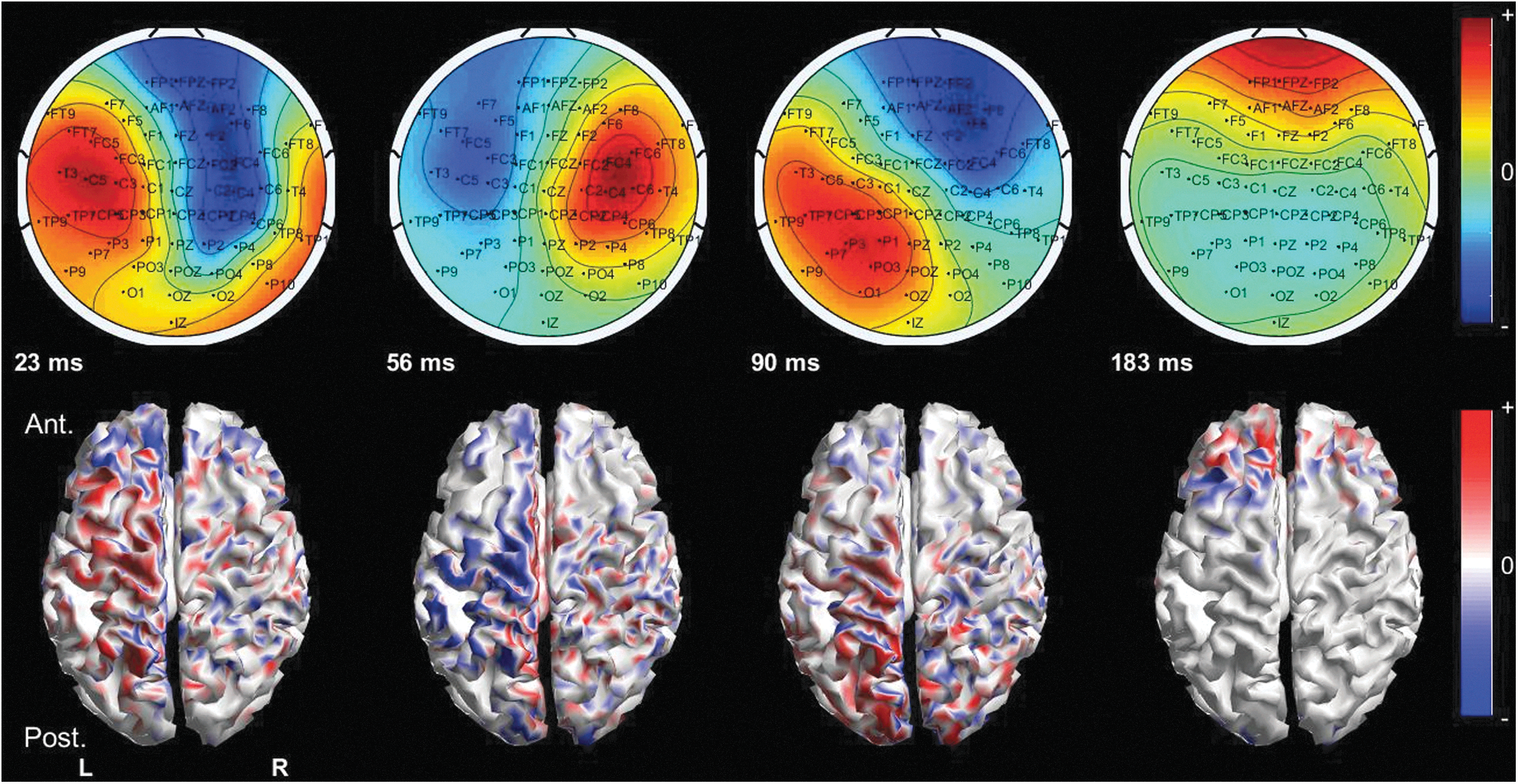
MNEs for the right M1 stimulation of S1. On the top row, the signal topography and, on the bottom row, the solutions of the MNEs for the given latency are shown. In the figures of the MNEs, the red and blue present primary currents directed outward and inward from the cortex, respectively. At 23 ms, the activation was strongest in the left frontoparietal area. At 56 ms, the posterior frontal and parieto-occipital areas were bilaterally activated, but the left hemisphere was more prominently activated. At 90 ms, the activation appeared again bilaterally in the posterior frontal and parieto-occipital areas with the dominance of the left hemisphere. At 183 ms, the activation was in the anterior frontal areas bilaterally, again with left dominance. MNEs, minimum-norm estimates.

FIG. 6.

Spreading of cortical activation after SMA stimulation. The first activity component appeared in the contralateral frontoparietal area in S1 and S2, and mainly in the frontal area in S3. The location of the second activity component differed between subjects. In S1, the strongest activity appeared in the contralateral parieto-occipital areas. In S2, the strongest activity was bilateral in the anterior frontal areas and, in S3, the strongest activity was contralateral in the frontal area. The third activity component appeared earlier in S1 than in S2 and S3. In S1, the activity appeared bilaterally with left dominance in the frontoparietal areas. The third activity component in S2 and S3 and the fourth activity component in S1 had almost the same latency. The strongest activity was bilateral in the frontal areas in S2, bilateral in the parieto-occipital areas in S3, and bilateral in the frontoparieto-occipital areas in S1. The fourth activity component appeared bilateral in the occipital areas in S3, and bilateral in the frontoparietal and parieto-occipital areas in S2, with left dominance.

Results

The latencies of GMFA peaks

The latencies of every GMFA peak from all subjects are shown in Table 1. The peaks with latencies near 50, 100, and 180 ms appeared most often and the peaks with latencies near 30 and 40 ms appeared most rarely. The peaks that were found in all three data sets (whole, odd, and even trials) were selected for source analysis.

Table 1.

The Latencies of All the Activation Peaks for Every Dataset

Activity peaks
No.	1	2	3	4	5	6
S1/M1		23^a		56^a	90^a	183^a
S1/PMd	16	28^a	43^a	63^a	106^a	137
S1/SMA	12^a	27^a	46^a	63	93^a	127
S2/M1	10	23^a	43^a	57^a	116^a	128
S2/PMd	8	25^a	41^a	63	91^a	181^a
S2/SMA	17		39^a	57^a	89^a	206^a
S3/M1	12^a		46^a	66^a	96^a	167
S3/PMd	17^a		46^a	66^a	95	152^a
S3/SMA	17	28^a		53^a	103^a	151^a

Peaks selected for further analysis.

M1, primary motor cortex; PMd, dorsal premotor area; SMA, supplementary motor area.

The spatial distribution of TEPs

The signal topographies and MNEs for the right M1 stimulation of S1 are presented in Figure 3.

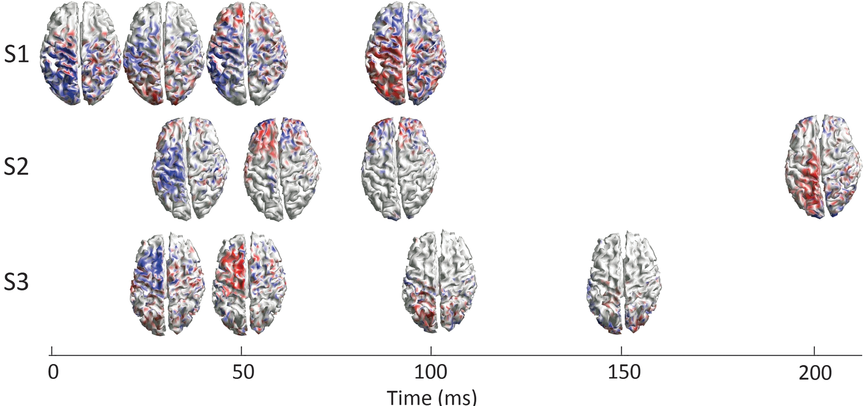
All 12 MNEs from the 3 subjects for the M1 stimulation are shown in Figure 4, presented on a timeline so that the TMS-induced activity patterns can be compared between subjects. The first two TEP components arose in the frontoparietal areas of the contralateral hemisphere in all subjects. The two last TEP components that had longer between-subject latency differences than the first two TEP components had more intersubject variability in the activity spreading.

FIG. 4.

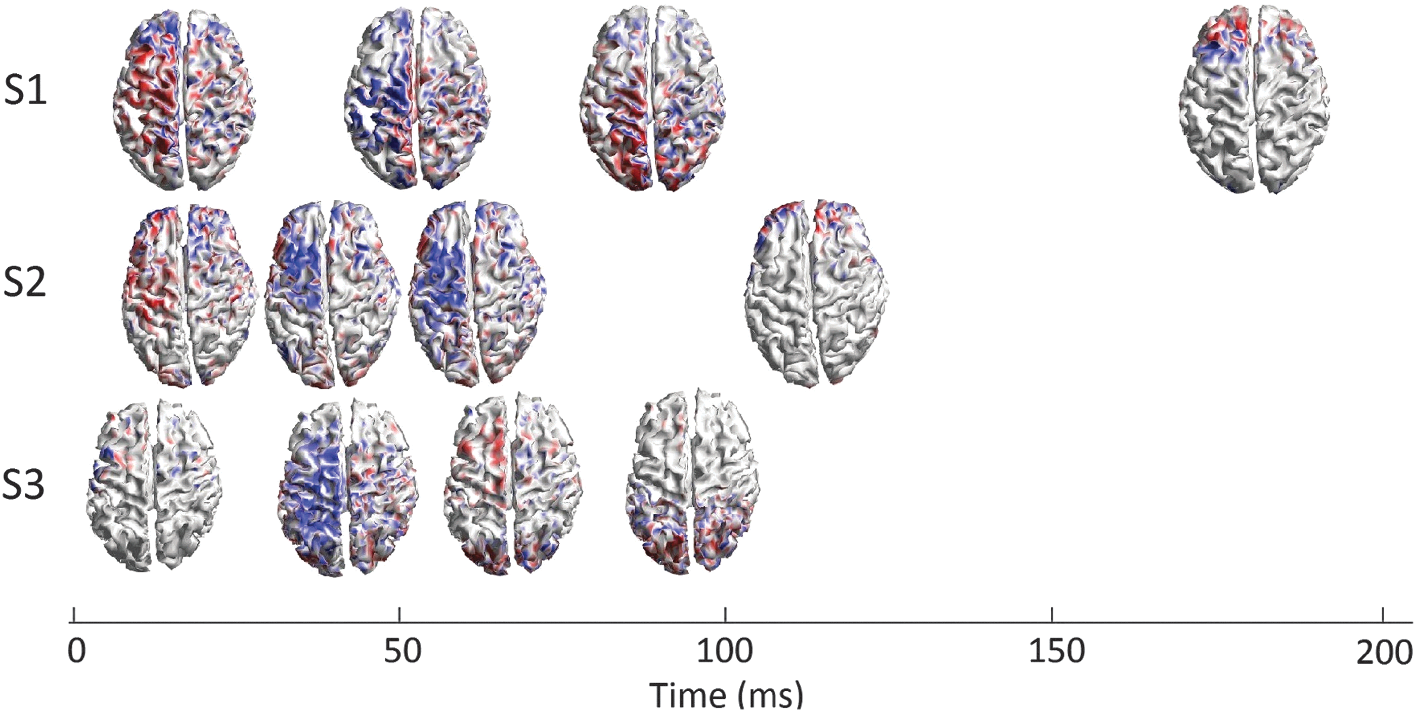
Spreading of cortical activation after the M1 stimulation. At first, the most prominent activity was in the frontal and parietal areas of the contralateral hemisphere in all subjects. The activity was weaker in S3 than in the other two subjects. The next activity peak appeared strongest in the posterior frontal or the frontoparietal areas, dominantly in the contralateral hemisphere. The latency of the third component was about 100 ms in S1, whereas in S2 and S3 the fourth component appeared with the latency of ∼100 ms. In S1, the activation appeared in a large area bilaterally, with the most prominent activity near the midline. In S2, the activity was focused in the frontal areas bilaterally, and in S3 in the posterior parietal and the occipital areas bilaterally. The fourth component in S1 appeared as late as 183 ms bilaterally in the frontal areas, with left dominance.

MNEs after the stimulation of the right PMd and right SMA are shown in Figures 5 and 6, respectively.

FIG. 5.

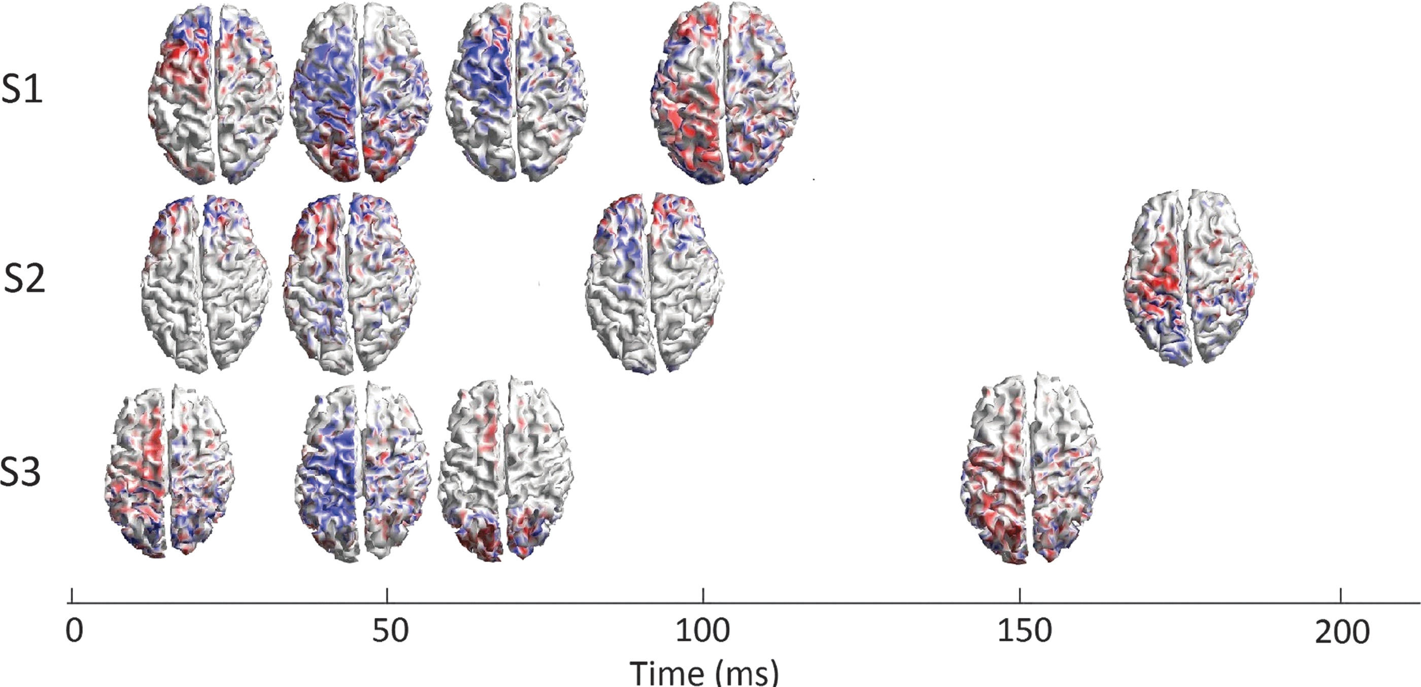
Spreading of cortical activation after PMd stimulation. At first, the activity arose in the bilateral frontal areas, with the most dominant activity in the contralateral hemisphere for S1 and S2. For S3, the contralateral medial frontal and central areas were activated first. For the second activity peak, the activation was strongest in the contralateral frontoparietal areas for S1 and S3 and the bilateral frontal areas for S2. There were larger latency differences between the third and fourth activity peaks among the subjects than between the first two TEP components. These latency differences were related to the more significant differences in the activity patterns. In S1 and S2, the third component appeared in the contralateral frontal areas, whereas in S3, it appeared in the contralateral medial frontal and the bilateral occipital areas. The fourth component was in the bilateral occipital areas in S3 and in the bilateral frontoparietal and parieto-occipital areas in S1 and contralateral frontoparietal and parieto-occipital areas in S2. TEP, TMS-evoked potential.

Discussion

We found that the order of activation of motor cortical areas depends on the stimulated area. The activation peak latencies and activation patterns varied between subjects also when the same target was stimulated. The similarities between subjects were found especially in the early activation patterns. Later patterns differed more, which can be explained partly by various TEP components having different latencies. According to previous studies, the late components have different generators; for example, N100 might be generated by TMS-induced cortical inhibition and P190 by the activation of the reverberant cortico-subcortical circuit (Bonato et al., 2006; Ferreri et al., 2011).

After the M1 stimulation, the spreading of activation was bilateral with principal activity in the contralateral hemisphere. In earlier TMS–EEG studies, the activation has been shown to be bilateral, appearing in the contralateral side in about 20 ms poststimulus (Bonato et al., 2006; Ilmoniemi et al., 1997; Komssi et al., 2002). The interhemispheric activation patterns may be due to propagation through the commissural pathways from M1 to the homologous contralateral cortical regions, to the contralateral SMA, and to PMd (Kandel and Schwartz, 1985). The intrahemispheric activation spreads may be related to the structural connections from the sensorimotor region near the hand representation area of M1 to SMA, the premotor cortex, and the somatosensory cortex (Guye et al., 2003; Kandel and Schwartz, 1985).

Massimini et al. (2005) found that the stimulation of PMd is transmitted to the contra- and bilateral frontal and parietal hemispheres. This is in line with our results even if the location of our PMd target differed from that of theirs, ours being located in a more caudal part of the PMd. Right PMd stimulation activated bilateral frontal areas first and then bilateral parietal areas, continuing with differing activation patterns between subjects, including frontal and parieto-occipital areas. Thus, we can say that later TEP components have fewer similarities in spatial distribution between subjects, probably due to activation through more complex neuronal networks, and that individual spreading is not always in line with spreading patterns found in group averages (Bonato et al., 2006; Komssi et al., 2002; Litvak et al., 2007).

SMA stimulation, similarly to M1 stimulation, resulted in early activation of contralateral frontoparietal areas. This might be explained by the caudal parts of SMA (SMA proper) having strong connections between ipsilateral M1 (Johansen-Berg et al., 2004) and the activation spreading to the contralateral hemisphere through ipsilateral M1.

In a recent TMS–EMG study, Fiori et al. (2017) studied interhemispheric connections from right M1 (rM1), right SMA (rSMA), right PM ventral (rPMv) and dorsal (rPMd) to left M1 by applying paired TMS pulses. They reported that the stimulation of TMS with a 40-ms ISI to rSMA, rM1, and rPMv induced inhibitory effects in the left M1 (Fiori et al., 2017). Similarly, we found that the stimulation of rM1 and rSMA induces cortical activity in the left central regions, that is, in frontoparietal areas after 40 ms of the stimulus, which was not seen as clearly when rPMd was stimulated.

Overall, the stimulations of M1 and SMA produced the first strong activation in the contralateral frontoparietal areas, and the stimulation of PMd in the contralateral prefrontal or frontoparietal areas, depending on the subject. The activation spreads of TEPs have been described before for M1 and prefrontal areas (George et al., 1999; Lioumis et al., 2009) and as shown here, TEPs spread differently when various cortical sites are stimulated with TMS or other cortical modulation technologies.

The results reported here underline the importance of studying the activation order of cortical and subcortical networks at individual level. Individual activation patterns may be used if, for example, damaged cortico-cortical connections are strengthened with a neuromodulation technique, such as cortico-cortical paired associative stimulation (ccPAS) (Veniero et al., 2013). ccPAS has been applied for instance to enhance motion sensitivity of vision by stimulating two connected targets in visual cortical areas with ISI of 20 ms (Romei et al., 2016). With the ccPAS protocol, long-term potentiation or long-term depression is proposed to be induced in synapses, representing spike-timing-dependent-plasticity (Veniero et al., 2013). In ccPAS, it is crucial to know the time interval between the activation of the second stimulation target and the stimulation of the first target so that the timing of the second pulse to the second target is correct to strengthen the synapses between the two targets (Veniero et al., 2013). Using TMS–EEG data to plan ccPAS protocols needs, however, to be carefully validated because the relationship between the observed TMS-evoked EEG responses and possible ccPAS protocols is not perfectly understood (Koch et al., 2013; Veniero et al., 2013). In addition to ccPAS, resting-state TMS–EEG results, as reported in this study, could be used as a control or baseline measurement if cortico-cortical network dynamics are studied, for example, in different cognitive tasks such as imagining movement.

The small sample size (N = 3) in our study restricts us from generalizing the obtained results to wider populations. With the small number of subjects, possible similarities in temporal and spatial distribution of TEPs across subjects may not arise as from larger amount of data and subjects. We found, however, that there are differences between subjects and we qualitatively characterized them. Studies that present results of activation spreading across different subjects must thus be interpreted carefully. Another limitation of our experiment is the uncertainty in knowing the location of the functional areas. As described, we selected the stimulation targets in the nonprimary motor areas by using anatomical cortical landmarks and in M1 by mapping the optimal hand muscle representation area. However, even if the same cortical areas were stimulated according to anatomical landmarks, the locations of the functional areas such as PMd and SMA are known to differ between individuals (Geyer, 2004; Geyer et al., 1996). Moreover, even if the same functional areas were stimulated, we do not know how the stimulation targets are related to the underlying axonal connections. These differences in the stimulation targets could also explain the different activity patterns found in our study. Individual tractography could help in finding similar TMS targets for PMd and SMA stimulations, with strong structural connections originating from the stimulation site.

The SI was determined individually to correspond to the generated E-field value of 90% of MT for all three stimulation sites. This quite low SI was selected to avoid muscle artifacts, but it might explain the weak responses (Kähkönen et al., 2004, 2005; Komssi et al., 2004); this may also be the reason for the lack of some typical TEP components. In our study, the stimulation of M1 produced larger GMFAs than stimulation of the other two sites in two out of three subjects. This effect was first reported by Kähkönen et al. (2005), who showed that the stimulation of the prefrontal areas produces weaker responses than the stimulation of M1. However, the GMFAs in S3 were almost equal for all stimulation sites. The GMFAs were quite low in S3 after the M1 stimulation, and background alpha oscillations may be superposed with the TEP components, which might be the reason for the occipital activity that appeared in S3.

Conclusions

We have shown how the spatial distribution of TEPs can be used to study effective connectivity originating from M1 and from nonprimary motor areas. There are similarities in the spreading of cortical activation, especially at short poststimulus latencies, and more differences at long latencies. The strength of the activation and the latencies between the activation peaks seen in GMFA differed between subjects, which may be related to the differences in the spatial activity patterns. Because of the small number of subjects, our results must be considered preliminary. Individual activity patterns could be determined if different neuromodulation techniques, such as ccPAS, were used to enhance cortico-cortical connections between remote cortical areas, especially outside M1. Although our study focused on motor-related areas, we might assume that connectivity profiles originating from nonmotor targets also differ between subjects.

Footnotes

Acknowledgments

This work was supported by the Maud Kuistila Memorial Foundation, the Ella and Georg Ehrnrooth Foundation, and the Academy of Finland. The authors thank Niko Mäkelä and Jaakko Nieminen for their assistance in the experimental setting and for comments on the project and Ville Mäntynen for his comments on the analysis.

Author Disclosure Statement

R.J.I. is founder, past CEO, advisor, and a minority shareholder of Nexstim Plc. The other authors declare no conflict of interest.

References

Arai

, Yoshikazu

. 2012. Effective connectivity between human supplementary motor area and primary motor cortex: a paired-coil TMS study. Exp Brain Res, 220:79–87.

Barker

, Jalinous

, Freeston

. 1985. Non-invasive magnetic stimulation of human motor cortex. Lancet, 1:1106–1107.

Bonato

, Miniussi

, Rossini

. 2006. Transcranial magnetic stimulation and cortical evoked potentials: a TMS/EEG co-registration study. Clin Neurophysiol, 117:1699–1707.

Bortoletto

, Veniero

, Thut

, Miniussi

. 2015. The contribution of TMS–EEG coregistration in the exploration of the human cortical connectome. Neurosci Biobehav Rev, 49:114–124.

Cona

, Semenza

. 2017. Supplementary motor area as key structure for domain-general sequence processing: a unified account. Neurosci Biobehav Rev, 72:28–42.

Delorme

, Makeig

. 2004. EEGLAB: an open sorce toolbox for analysis of single-trial EEG dynamics including independent component analysis. J Neurosci Methods, 134:9–21.

Di Lazzaro

, Oliviero

, Profice

, Saturno

, Pilato

, Insola

, et al. 1998. Comparison of descending volleys evoked by transcranial magnetic and electric stimulation in conscious humans. Electroencephalogr Clin Neurophysiol, 109:397–401.

Di Lazzaro

, Rothwell

, Capogna

. 2017. Noninvasive stimulation of the human brain: activation of multiple cortical circuits. Neuroscientist, 24:246–260.

Di Lazzaro

, Ziemann

. 2013. The contribution of transcranial magnetic stimulation in the functional evaluation of microcircuits in human motor cortex. Front Neural Circuits, 7:1–9.

10.

Ferbert

, Priori

, Rothwell

, Day

, Colebatch

, Marsden

. 1992. Interhemispheric inhibition of the human motor cortex. J Physiol, 453:525–546.

11.

Ferreri

, Pasqualetti

, Määttä

, Ponzo

, Ferrarelli

, Tononi

, et al. 2011. Human brain connectivity during single and paired pulse transcranial magnetic stimulation. Neuroimage, 54:90–102.

12.

Ferreri

, Pauri

, Pasqualetti

, Fini

, Dal Forno

, Rossini

. 2003. Motor cortex excitability in Alzheimer's disease: a transcranial magnetic stimulation study. Ann Neurol, 53:102–108.

13.

Fiori

, Chiappini

, Candidi

, Romei

, Borgomaneri

, Avenanti

. 2017. Long-latency interhemispheric interactions between motor-related areas and the primary motor cortex: a dual site TMS study. Sci Rep, 7:1–10.

14.

Fischl

, Salat

, Busa

, Albert

, Dieterich

, Haselgrove

, et al. 2002. Whole brain segmentation: neurotechnique automated labeling of neuroanatomical structures in the human brain. Neuron, 33:341–355.

15.

Fox

, Narayana

, Tandon

, Sandoval

, Fox

, Kochunov

, Lancaster

. 2004. Column-based model of electric field excitation of cerebral cortex. Hum Brain Mapp, 22:1–14.

16.

George

, Stallings

, Speer

, Nahas

, Spicer

, Vincent

, et al. 1999. Prefrontal repetitive transcranial magnetic stimulation (rTMS) changes relative perfusion locally and remotely. Hum Psychopharmacol Clin Exp, 14:161–170.

17.

Geyer

. 2004. The microstructural border between the motor and the cognitive domain in the human cerebral cortex. Adv Anat Embryol Cell Biol, 174:I–VIII, 1–89.

18.

Geyer

, Ledberg

, Schleicher

, Kinomura

, Schormann

, Burgel

, et al. 1996. Two different areas within the primary motor cortex of man. Nature, 382:805–807.

19.

Guye

, Parker

GJM

, Symms

, Boulby

, Wheeler-Kingshott

CAM

, Salek-Haddadi

, et al. 2003. Combined functional MRI and tractography to demonstrate the connectivity of the human primary motor cortex in vivo. Neuroimage, 19:1349–1360.

20.

Hallett

. 2000. Transcranial magnetic stimulation and the human brain. Nature, 406:147–150.

21.

Hämäläinen

, Ilmoniemi

. 1994. Interpreting magnetic fields of the brain: minimum norm estimates. Med Biol Eng Comput, 32:35–42.

22.

Ilmoniemi

, Karhu

. 2012. TMS and electroencephalography: methods and current advances. In: Epstein

, Wassermann

, Ziemann

(eds.) Oxford Handbook of Transcranial Stimulation. New York, NY: Oxford University Press Inc.; pp. 593–608.

23.

Ilmoniemi

, Virtanen

, Ruohonen

, Karhu

, Aronen

, Naatanen

, Katila

. 1997. Neuronal responses to magnetic stimulation reveal cortical reactivity and connectivity. Neuroreport, 8:3537–3540.

24.

Johansen-Berg

, Behrens

TEJ

, Robson

, Drobnjak

, Rushworth

MFS

, Brady

, et al. 2004. Changes in connectivity profiles define functionally distinct regions in human medial frontal cortex. Proc Natl Acad Sci U S A, 101:13335–13340.

25.

Kähkönen

, Komssi

, Wilenius

, Ilmoniemi

, Ka

, Kähkönen

, et al. 2005. Prefrontal transcranial magnetic stimulation produces intensity-dependent EEG responses in humans. Neuroimage, 24:955–60.

26.

Kähkönen

, Wilenius

, Komssi

, Ilmoniemi

. 2004. Distinct differences in cortical reactivity of motor and prefrontal cortices to magnetic stimulation. Clin Neurophysiol, 115:583–588.

27.

Kandel

, Schwartz

. 1985. Principles of Neural Science. New York, NY: Elsevier.

28.

Koch

, Ponzo

, Di Lorenzo

, Caltagirone

, Veniero

. 2013. Hebbian and anti-hebbian spike-timing-dependent plasticity of human cortico-cortical connections. J Neurosci, 33:9725–9733.

29.

Komssi

, Aronen

, Huttunen

, Kesäniemi

, Soinne

, Nikouline

, et al. 2002. Ipsi- and contralateral EEG reactions to transcranial magnetic stimulation. Clin Neurophysiol, 113:175–184.

30.

Komssi

, Kähkönen

. 2006. The novelty value of the combined use of electroencephalography and transcranial magnetic stimulation for neuroscience research. Brain Res Rev, 52:183–192.

31.

Komssi

, Kähkönen

, Ilmoniemi

. 2004. The effect of stimulus intensity on brain responses evoked by transcranial magnetic stimulation. Hum Brain Mapp, 21:154–164.

32.

Kujirai

, Caramia

, Rothwell

, Day

, Thompson

, Ferbert

, et al. 1993. Corticocortical inhibition in human motor cortex. J Physiol, 471:501–519.

33.

Lee

, Harrison

, Mechelli

. 2003. A report of the functional connectivity workshop, Dusseldorf 2002. Neuroimage, 19:457–465.

34.

Lehmann

, Skrandies

. 1980. Reference-free identification of components of checkerboard-evoked multichannel potential fields. Electroencephalogr Clin Neurophysiol, 48:609–621.

35.

, Song

, Fan

, Liu

, Jiang

. 2015. Parcellation of the primary cerebral cortices based on local connectivity profiles. Front Neuroanat, 9:50.

36.

Lin

F-H

, Belliveau

, Dale

, Hämäläinen

. 2006. Distributed current estimates using cortical orientation constraints. Hum Brain Mapp, 27:1–13.

37.

Lioumis

, Kicic

, Savolainen

, Makela

, Kahkonen

. 2009. Reproducibility of TMS-evoked EEG responses. Hum Brain Mapp, 30:1387–1396.

38.

Litvak

, Komssi

, Scherg

, Hoechstetter

, Classen

, Zaaroor

, et al. 2007. Artifact correction and source analysis of early electroencephalographic responses evoked by transcranial magnetic stimulation over primary motor cortex. Neuroimage, 37:56–70.

39.

Massimini

, Ferrarelli

, Huber

, Esser

, Singh

, Tononi

. 2005. Breakdown of cortical effective connectivity during sleep. Science, 309:2228–2232.

40.

Matsuura

, Okabe

. 1995. Selective minimum-norm solution of the biomagnetic inverse problem. IEEE Trans Biomed Eng, 42:608–615.

41.

Mutanen

, Mäki

, Ilmoniemi

. 2013. The effect of stimulus parameters on TMS–EEG muscle artifacts. Brain Stimul, 6:371–376.

42.

Mutanen

, Kukkonen

, Nieminen

, Stenroos

, Sarvas

, Ilmoniemi

. 2016. Recovering TMS-evoked EEG responses masked by muscle artifacts. Neuroimage, 139:157–166.

43.

Mutanen

, Metsomaa

, Liljander

, Ilmoniemi

. 2018. Automatic and robust noise suppression in EEG and MEG: the SOUND algorithm. Neuroimage, 166:135–151.

44.

Nakamura

, Kitagawa

, Kawaguchi

, Tsuji

. 1996. Direct and indirect activation of human corticospinal neurons by transcranial magnetic and electrical stimulation. Neurosci Lett, 210:45–48.

45.

Nikouline

, Ruohonen

, Ilmoniemi

. 1999. The role of the coil click in TMS assessed with simultaneous EEG. Clin Neurophysiol, 110:1325–1328.

46.

Orgogozo

, Larsen

. 1979. Activation of the supplementary motor area during voluntary movement in man suggests it works as a supramotor area. Science, 206:847–850.

47.

Penfield

, Jasper

. 1954. Epilepsy and the Functional Anatomy of the Human Brain. Boston, MA: Little, Brown.

48.

Penfield

, Welch

. 1951. The supplementary motor area of the cerebral cortex: a clinical and experimental study. AMA Arch Neurol Psychiatry, 66:289–317.

49.

Picard

, Strick

. 2001. Imaging the premotor areas. Curr Opin Neurobiol, 11:663–672.

50.

Raz

, Turetsky

, Fein

. 1988. Confidence intervals for the signal-to-noise ratio when a signal embedded in noise is observed over repeated trials. IEEE Trans Biomed Eng, 35:646–649.

51.

Romei

, Chiappini

, Hibbard

, Avenanti

. 2016. Empowering reentrant projections from V5 to V1 boosts sensitivity to motion. Curr Biol, 26:2155–2160.

52.

Rossini

, Rossi

. 2007. Transcranial magnetic stimulation: diagnostic, therapeutic, and research potential. Neurology, 68:484–488.

53.

Sarvas

. 1987. Basic mathematical and electromagnetic concepts of the biomagnetic inverse problem. Phys Med Biol, 32:11–22.

54.

Shattuck

, Leahy

. 2002. BrainSuite: an automated cortical surface identification tool. Med Image Anal, 6:129–142.

55.

Stenroos

, Sarvas

. 2012. Bioelectromagnetic forward problem: isolated source approach revis(it)ed. Phys Med Biol, 57:3517–3535.

56.

Thielscher

, Opitz

, Windhoff

. 2011. Impact of the gyral geometry on the electric field induced by transcranial magnetic stimulation. Neuroimage, 54:234–243.

57.

Veniero

, Ponzo

, Koch

. 2013. Paired associative stimulation enforces the communication between interconnected areas. J Neurosci, 33:13773–13783.

58.

Virtanen

, Ruohonen

, Näätänen

, Ilmoniemi

. 1999. Instrumentation for the measurement of electric brain responses to transcranial magnetic stimulation. Med Biol Eng Comput, 37:322–326.

Individual Activation Patterns After the Stimulation of Different Motor Areas: A Transcranial Magnetic Stimulation–Electroencephalography Study

Abstract

Introduction

Materials and Methods

Subjects

EEG, EMG, and TMS

Stimulation sites

Stimulation parameters

Computation of the lead fields

Data processing

Signal analysis

Minimum-norm estimation

Spatial distribution

Results

The latencies of GMFA peaks

The spatial distribution of TEPs

Discussion

Conclusions

Footnotes

Acknowledgments

Author Disclosure Statement

References