Identification of Subclinical Language Deficit Using Machine Learning Classification Based on Poststroke Functional Connectivity Derived from Low Frequency Oscillations

Abstract

Post-stroke neuropsychological evaluation is time-intensive in assessing impairments in subjects without overt clinical deficits. We utilized functional connectivity (FC) from ten-minute non-invasive resting-state functional MRI (rs-fMRI) to identify stroke subjects at risk for subclinical language deficit (SLD) using machine learning. Discriminative ability of FC derived from slow-5 (0.01–0.027 Hz), slow-4 (0.027–0.073 Hz) and low frequency oscillations (LFO; 0.01–0.1 Hz) was compared. Sixty clinically non-aphasic right-handed subjects were categorized into three subgroups based on stroke status and normalized verbal fluency (NVF) score: 20 ischemic early-stage stroke subjects at higher risk for SLD (LD+; mean VFS=−1.77), 20 ischemic early-stage stroke subjects with at risk for SLD (LD-; mean VFS=−0.05), 20 healthy controls (HC; mean VFS=0.29). T1-weighted and rs-fMRI were acquired within 30 days of stroke onset. Blood-oxygen-level-dependent signal was extracted within the language network. FC was evaluated and used by a multiclass support vector machine to classify test subject into a subgroup which was assessed by nested leave-one-out cross-validation. FC derived from slow-4 (70%) provided the best accuracy relative to LFO (65%) and slow-5 (50%), reasonably higher than random chance (33.33%). Using subgroup-specific accuracy, classification was best realized within slow-4 for LD+ (81.6%) and LD- (78.3%) and slow-4/LFO for HC (80%), i.e., early-stage stroke subjects showed a slow-4 FC dominance whereas HC also indicated the normalized involvement within LFO. While frontal FC differentiated stroke from healthy, occipital FC differentiated between the two stroke subgroups. Thus, stroke subjects at risk for SLD can be identified using rs-fMRI reasonably in an expedited manner.

Introduction

Background

Stroke is typically associated with high rates of morbidity, mortality and high levels of disability (e.g., loss in motor, speech, cognitive, and visual functions) in survivors. The degree of impairment is largely determined by severity of stroke. On one hand, clinical deficits are severe impairments, easier to diagnose, and well understood. On the other hand, subclinical deficits are milder forms of impairments, harder to identify, and have been paid limited attention to in the literature. While subclinical deficits resulting from neurological diseases might not significantly deter normal brain functions, they may still impact the quality of life of the survivor in the long run. This has been shown for cognitive domains (Mitchell et al., 2010) and might be extended to the noncognitive domains of the brain as well.

Behavioral and neuropsychological assessments (Ivnik et al., 1996) serve as a medium to identify the extent of impairments caused due to the occurrence of stroke (Patterson, 2011; Szaflarski et al., 2011). Such assessments are especially important to identify subclinical impairments. This typically requires administration of a battery of tests, tasks, and questionnaires by a trained professional to evaluate poststroke brain functions. The scores achieved by the subject on these tests reflect the areas and degrees of impairments. While the neuropsychological examinations are very detailed and helpful in determination of extent of deficits, the administration and assessment can be a time-intensive process.

Our goal was to assess if neuroimaging methods can provide information, equivalent or supplementary, to neuropsychological testing in terms of diagnosing poststroke subclinical deficits. Specifically, we tested this for the language domain in stroke survivors relative to control subjects within stroke, as well as healthy, populations. To this end, it is important to choose a suitable modality of imaging to use and the specific information to be extracted from it. A convenient method is resting-state functional magnetic resonance imaging (rs-fMRI), which is noninvasive, time-efficient, and task-free for the subjects. Examination of network-based functional connectivity (FC) could additionally narrow down the search for specific subclinical deficits among stroke survivors.

Related work and motivation

From the perspective of neuroimaging, overt clinical poststroke impairments and recovery in various domains such as cognition, motor, language, emotion, and so on are largely well explored (Nys et al., 2005; Ochsner et al., 2002; Ward et al., 2003). However, limited studies have examined the subclinical impairments following stroke. While many studies have delved deep into discerning the nature of mild impairments in cognitive brain functions (Dickerson et al., 2005; Hämäläinen et al., 2007; Rombouts et al., 2005) due to association with dementia and Alzheimer's disease, such subclinical impairments may or may not be the consequence of stroke. Several studies have examined mild deficits occurring after stroke and are limited to mainly cognitive or motor domains (Hommel et al., 2009; Rosso et al., 2013; Schaechter, 2004; Stephens et al., 2005).

Relatively fewer studies have analyzed mild impairments in language network following stroke (Mohanty et al., 2018; Nair et al., 2015). We add to this by presenting a rs-fMRI based approach to analyze subclinical deficits in the language domain in sample stroke subjects. Low frequency blood-oxygen-level dependent (BOLD) fluctuations are typically extracted from rs-fMRI in the frequency range of 0.01–0.1 Hz to filter out the effect of physiological noise (Biswal et al., 1995). Based on electrophysiological studies, this frequency band is further subdivided into multiple bands, that is, slow-5 (0.01–0.027 Hz), slow-4 (0.027–0.073 Hz), and partially slow-3 (0.073–0.198 Hz; Buzsáki and Draguhn, 2004; Penttonen and Buzsáki, 2003). Specifically, gray matter corresponds to the slow-4 and slow-5 bands, while slow-3 and slow-2 (0.198–0.25 Hz) have been typically associated with signals arising due to respiratory cardiac processes and linked to white matter (Zuo et al., 2010).

Traditional metrics used to study frequency fluctuations in stroke population are amplitude of low-frequency fluctuation (ALFF), fractional ALFF (La et al., 2016a,b), and regional homogeneity (ReHo) (Tang et al., 2016). Recently Gohel and Biswal (2015) suggested that rs-fMRI exhibits FC distributed over multiple frequency bands in healthy adults. While this multiband FC approach has also been demonstrated in epileptic population (Hwang et al., 2019) and in population with vascular dementia (Zhang et al., 2013) using machine learning classification, similar effects have not been documented in case of stroke population. These factors serve as the primary motivation for the current study.

Overview of this study

In this study, we focused on identification of subclinical deficits at an early-stage (within 30 days of stroke onset) after stroke by examining neuroimaging data in place of commonly used neuropsychological test scores. Specifically, we demonstrated, using rs-fMRI, that cases of subclinical language deficit (SLD) can be differentiated from the cases without SLD. This was achieved by evaluating the resting-state FC in the language network. While FC is most commonly evaluated in the low frequency oscillation (LFO; 0.01–0.1 Hz), motivated by the evidence on the multiband phenomenon of FC described in the previous section, we examined two subset bands namely slow-4 and slow-5 to test their discriminative powers in identification of SLD. A multiclass support vector machine (SVM) based machine learning classifier was used to identify specific brain regions and connections between stroke subjects with and without SLD. In addition, a third group of healthy subjects was included as a control group to account for changes in FC due to normal aging.

The significance of this work is threefold: (1) findings suggest that task-free imaging such as rs-fMRI, acquired in a span of about 10 min, could provide useful information to identify SLD, which otherwise takes longer to assess using neuropsychological assessments; (2) results demonstrate that FC derived from slow-4 band that corresponds to the gray matter in the brain is more relevant and informative than the conventionally used FC in LFO or slow-5 bands to study stroke population; and (3) the distinction between the presence or absence of SLD can be automated with a high performance machine learning classifier.

Methods

Subjects

Sixty subjects were recruited as a part of an ongoing longitudinal study investigating neuroplasticity and recovery in stroke survivors. The cohort consisted of three subgroups formed on the basis of stroke status and normalized score on the verbal fluency (NVF) behavioral task:

20 ischemic early-stage stroke subjects at a higher risk of SLD (LD⁺)

20 ischemic early-stage stroke subjects at a lower risk of SLD (LD⁻)

20 healthy control (HC) subjects

The inclusion criteria for enrollment of stroke subjects in this study were as follows: 18 years or older with ischemic stroke and ability to provide written consent. The lower age limit of 18 years was the only inclusion criterion for enrollment of healthy subjects in the study. The exclusion criteria for the study were as follows: subjects with contraindications for MRI, such as having pacemakers, defibrillator, aneurysm clips, metallic components, and so on, and subjects under certain types of medication for psychiatric illness or confounding neurological disorders and subjects with history of drug abuse.

The group membership of the stroke subjects to LD⁺ or LD⁻ was determined based on a median-split of collective NVF scores of the 40 stroke subjects. The reason for enrollment of healthy subjects was to enable comparison of the deficits observed in stroke subjects with matched controls so that effects due to normal aging are taken into account. The sample characteristics of the subjects are listed in Table 1. Subjects were age, gender, and education matched across the three subgroups. Time since stroke was calculated as the time period between stroke onset and the date of scan. Lesion hemisphere was determined based on the scan by a neuroradiologist to be left (L), right (R), or bilateral (B). Stroke severity was based on National Institute of Healthy Stroke Scale (NIHSS) score and was trichotomized into: (1) minor (NIHSS = 0–4); (2) moderate (NIHSS = 5–16); and (3) missing (NIHSS not available).

Table 1.

Study Sample Characteristics

	LD⁺			LD⁻			HC
Sample size	20			20			20
Handedness	R			R			R
Age (mean age ± SD)	58.35 ± 15.23			63.10 ± 12.59			57.85 ± 7.75
Gender (male/female)	12/8			15/5			11/9
Education (mean years ± SD)	14.84 ± 2.71			14.84 ± 2.26			16.5 ± 3.13
Lesion hemisphere	L	R	B	L	R	B	N/A
Lesion hemisphere	14	6	0	10	7	3	N/A
Stroke severity	Min	Mod	Miss	Min	Mod	Miss	N/A
Stroke severity	15	3	2	18	1	1	N/A
Time since stroke (mean days ± SD)	7.15 ± 3.67			8.45 ± 9.62			N/A
NVF score (mean NVF ± SD)	−1.776 ± 0.62			−0.05 ± 0.53			0.29 ± 0.97

The three subgroups are: LD⁺ (stroke subgroup at higher risk of SLD), LD⁻ (stroke subgroup at lower risk of SLD), and HC (healthy control) subgroup. NVF refers to the normalized verbal fluency score as measured by COWAT during behavioral testing outside the scanner. Lesion hemisphere: L, left; R, right; B, bilateral. Stroke severity: Min, minor; Mod, moderate; Miss, missing.

N/A, not applicable; SD, standard deviation.

The study was conducted in accordance with protocol approved by the local Health Sciences Institutional Review Board. All subjects provided written informed consent. All subjects were clinically nonaphasic. In addition, for the purposes of this analysis, only right-handed subjects were chosen since language network in the brain could be lateralized depending upon handedness (Knecht et al., 2000).

Data acquisition: neuroimaging and behavioral data

Five-minute structural MRI scans were acquired on 3T GE 750 scanners (GE Healthcare, Waukesha, WI) equipped with an eight-channel head coil. These were T1-weighted axial anatomical scans and were collected using FSPGR BRAVO sequence with the following specifications: repetition time (TR) = 8.132 ms, echo time (TE) = 3.18 ms, inversion time (TI) = 450 ms over a 256 × 256 matrix and 156 slices, flip angle = 12, field of view (FOV) = 25.6 cm, slice thickness = 1 mm. Rs-fMRI was collected with subjects lying in the scanner eyes closed lasting about 10 min. Rs-fMRI was obtained using single-shot echo-planar T2*-weighted imaging with the following parameters: TR = 2.6 sec, 231 time points, TE = 22 ms, FOV = 22.4 cm, flip angle = 60, voxel dimensions 3.5 × 3.5 × 3.5 mm³, and 40 slices. Assessment of SLD was based on verbal fluency task administered outside the scanner during behavioral testing by conducting the Controlled Oral Word Association Test (Ruff et al., 1996). The scores obtained on this test facilitate detection of disorders and characterization of the language network in the brain.

Data preprocessing: neuroimaging data

Subjects were chosen so that their scans were free of any obvious artifacts upon visual inspection. Rs-fMRI data were processed using AFNI (Cox, 1996). For fMRI, the first 3 volumes were discarded, rest of the volumes were despiked to truncate spikes in time course of each voxel arising due to motion, slice time corrected with the initial volume as the reference, aligned with the structural scan, normalized to the standard Montreal Neurological Institute (MNI) space, censored for motion (based on the Euclidean norm computed from motion parameters and derivatives; threshold = 0.25 mm), and bandpass filtered simultaneously, spatially smoothed with a 4-mm full-width-half-maximum Gaussian kernel based on a prior similar study (Nair et al., 2015).

Motion-based volume removal was performed when more than 10% of the automasked brain was deemed outliers. Regression of motion parameters, derivatives of motion parameters, rate of change of BOLD signal (DVARS), and white matter and cerebrospinal fluid signals were performed simultaneously in a single general linear regression model. The bandpass filtering was focused to the three frequency bands of interest: the conventional LFO (0.01–0.1 Hz), slow-4 (0.027–0.073 Hz), and slow-5 (0.01–0.027 Hz) frequency bands. This resulted in three sets of data that were separately analyzed and compared. Global signal regression was omitted due to the controversial position associated with it in the literature (Murphy and Fox, 2016).

Data preprocessing: behavioral data

Raw values of scores achieved on the verbal fluency task were corrected for age and education as proposed by Tombaugh et al. (1999). The raw score was transformed as follows: \documentclass{aastex}\usepackage{amsbsy}\usepackage{amsfonts}\usepackage{amssymb}\usepackage{bm}\usepackage{mathrsfs}\usepackage{pifont}\usepackage{stmaryrd}\usepackage{textcomp}\usepackage{portland, xspace}\usepackage{amsmath, amsxtra}\usepackage{upgreek}\pagestyle{empty}\DeclareMathSizes{10}{9}{7}{6}\begin{document} \begin{align*} \textbf{\textit {NVF}} = \frac{\textbf{\textit{RVF}}-\textbf{\textit {M}}} {\textbf{\textit{SD}}} , \end{align*} \end{document}

where NVF is the normed verbal fluency score (VFS), RVF is the raw VFS, M is the mean percentile score specific to the age group and level of education, and SD is the standard deviation percentile score specific to the age group and level of education.

Seed-based functional connectivity

Since this work was focused on the language network, a seed-based FC approach was adopted. Based on a prior study (Tomasi and Volkow, 2012), 23 seed regions of interest (ROIs) were chosen. This ROI template provides coverage of brain regions responsible for multiple aspects of language processing such as phonological and lexical-semantic functions, speech comprehension, and production. The MNI coordinates of the seeds are listed in Table 2 and visualized in Figure 1 using BrainNet Viewer (Xia et al., 2013). Spherical seeds at the specified MNI coordinates were created, each of radius 6 mm for each subject. This template was applied to the spatially normalized residuals of the resting data, and BOLD time series was extracted at each ROI. A correlation matrix of size 23-by-23 was generated by temporally correlating time series from pairs of seeds. Of the 529 total correlation coefficients, 253 unique coefficients were retained for analysis, and duplicates were discarded. Sample correlation matrices are presented in Figure 2e. This process was replicated for each subject and for each frequency band.

FIG. 1.

The 23 ROIs used for the language network in this study are plotted. The labels corresponding to the numbering can be found in Table 2. ROIs, regions of interest.

FIG. 2.

Methodology for single subject analysis: (a) raw structural T1 scan (left) and T1 scan spatially normalized to MNI space (right); (b) raw functional scan (left) and preprocessed up to smoothing (right); (c) smoothed fMRI is temporally filtered in the LFO (top), slow-4 (center), slow-5 (bottom) bands; (d) 23 ROIs of the language network used to extract BOLD time courses for each of the three frequency bands; (e) 23 × 23 FC matrix computed for LFO (top), slow-4 (center), and slow-5 (bottom) bands; (f) FC matrix reduced to 253-dimensional vector constituting of unique correlation coefficients between pairs of ROIs. BOLD, blood-oxygen-level dependent; FC, functional connectivity; fMRI, functional magnetic resonance imaging; LFO, low frequency oscillation; MNI, Montreal Neurological Institute.

Table 2.

Regions of Interest Encompassing the Language Network are Presented Along with the Brodmann Area They Belong to and Their Standard Montreal Neurological Institute Coordinates

ID	Brain region	Brodmann area	x (mm)	y (mm)	z (mm)
1	Broca's area	45	−51	27	18
2	L Caudate	—	−12	9	15
3	R Caudate	—	12	12	12
4	Cerebellum	crus	15	−81	−30
5	Cingulate	24	0	0	48
6	Extrastriate	18	21	−69	−15
7	Inferior parietal	40	57	−51	36
8	L Inferior temporal	21/20	−57	−30	−15
9	R Inferior temporal	21/20	63	−30	−12
10	Middle frontal	46	−39	18	45
11	Pars opercularis	44	42	21	42
12	L Pars orbitalis	47	−45	39	−12
13	R Pars orbitalis	47	45	39	−15
14	Pars triangularis	45	51	30	18
15	Posterior parietal	7	6	−81	45
16	Putamen/globus pallidus	—	−18	0	9
17	Striate	17	6	−75	−6
18	Superior frontal	8	−3	36	45
19	Superior parietal	5	3	−51	57
20	L Superior temporal	42	−63	−18	9
21	R Superior temporal	42	60	−21	12
22	Ventral thalamus	—	−9	−9	0
23	Wernicke's area	39/40	−51	−51	30

ROIs in left and right hemispheres are prefixed by L and R, respectively. Anatomical locations are depicted in Figure 1.

ROIs, regions of interest.

Data analysis: sample characteristics

The subjects were chosen so as to have similar distributions in terms of age, gender, and education levels across the three subgroups. A two-sample t-test was carried out to identify any group differences in terms of age, education levels, time since stroke, and NVF. Since gender is a categorical variable, Fisher exact test was performed to study group differences. All tests were performed between pairs of subgroups. A number of metrics were evaluated for the purposes of quality control and to measure the impact of head motion on subsequent FC measures. We compared the six directional motion parameters obtained during motion correction from preprocessing (Cox and Jesmanowicz, 1999; Friston et al., 1995), frame-wise displacement to measure change in position of the head based on the derivatives of the motion parameters (Power et al., 2012), DVARS index to capture the rate of change of BOLD signal intensity (Smyser et al., 2010), and the temporal signal-to-noise ratio (Van Dijk et al., 2012).

Data analysis: group classification

Machine learning classification algorithms such as SVMs have been shown to have reasonably reliable performance with FC data (Dosenbach et al., 2010; Mohanty et al., 2018; Vergun et al., 2013). We adopted a similar paradigm but expanded it further by implementing multiclass linear-kernel SVM to perform classification among the classes: LD⁺, LD⁻, and HC based on a one-versus-one coding scheme. Since classification can be influenced by the number of features with respect to the sample size, we compared the performance with and without feature selection procedures. Appropriate feature selection can enhance classification accuracy by limiting the data to useful information (Demirhan et al., 2015).

Outlier removal

Before training a classifier, to ensure that the FC features were not impacted by outliers, an outlier removal step was deployed over all the features. Any value that was more than three scaled median absolute deviations (MADs; Leys et al., 2013) away from the median was deemed an outlier and was removed. This was repeated for features of each subgroup, and all possible outlier features were eliminated retaining common features across all subgroups.

Feature selection

FC features were ranked by importance depending upon their contribution toward the classification with a feature selection procedure. The aim of this step was to narrow down the search to a smaller subset of important features which can achieve a good classification performance. A neighborhood component analysis (NCA) algorithm (Goldberger et al., 2005) facilitated selection of features as it does not assume any parametric distribution of the features and is also suitable for multiclass classification using high dimensional features (Yang et al., 2012). This method learns weights corresponding to each feature while minimizing the cross-validation error. The features assigned with nonzero weights were then retained and fed into a multiclass SVM for classification among subgroups.

Model parameter optimization

The hyperparameters namely the misclassification cost and kernel scale corresponding to the classifier were optimized with a Bayesian optimization (Snoek et al., 2012) approach to prevent overfitting. By minimizing the cross-validation error over a range of values for 30 iterations, the optimal parameter values were obtained.

Classification

The goal of the current study is to be able to classify a given subject into one of the groups based on the selected FC data as representative features. A three-class linear-kernel SVM (Cortes and Vapnik, 1995) was applied due to the advantage of ease of interpretation of results. The data were standardized so that each feature had the same mean and variance to avoid one feature from dominating others due to a large magnitude. Since the dataset consists of three classes (LD⁺, LD⁻, and HC), the identification of SLD was modeled as a multi-(three)class problem (Allwein et al., 2000). A one-versus-one scheme was adopted which follows a pairwise decomposition (Knerr et al., 1990), within which all possible pairwise classifiers were trained and evaluated. This means that individual binary classifiers to differentiate between LD⁺ versus LD⁻, LD⁻ versus HC, and HC versus LD⁺ were considered. This was adopted over one-versus-all approach because one-versus-all would lead to an imbalance in class representation for our FC data. Each learned binary classifier is applied to the test sample, and the winning class gets one vote. Finally, the test sample was labeled to the class that received the most number of votes.

Cross-validation

A nested leave-one-out cross-validation (LOOCV; Cawley and Talbot, 2010; Hastie et al., 2001) was adopted to estimate classifier performance as it provides an unbiased approximation of the test error and is more suitable for a dataset with limited number of samples such as here. In the inner loop of this LOOCV, feature selection was performed by training and validation based on the NCA approach described above. The winning model from the inner loop corresponded to the one that used the minimum number of features to avoid overfitting and predicted maximum posterior probability. The outer loop of LOOCV optimized the validated winning model from the inner loop by tuning the hyperparameters, tested the new or unseen data, and was used to evaluate the quality of classifier performance. Since the training and testing data subsets are completely independent, nested cross-validation avoided learning an over optimistic model and provided generalizable classifier performance (Cawley and Talbot, 2010).

Feature contribution

Once a model was learned with optimal parameters, the use of a linear-kernel SVM enabled analysis of individual feature importance. The most discriminatory features were the FC connections, which were involved in classification of each left out sample during independent testing in the outer loop of nested cross-validation. The learned classifier model yielded a weighting coefficient corresponding to each of the selected features from the NCA model, whose magnitude was proportional to the importance of the features in discriminating between subgroups. These weights for the FC features were used to determine the weights of the involved ROIs (Dosenbach et al., 2010; Meier et al., 2012).

Overview of methodology

Overall, we learned optimized classification models using FC in each frequency band, identified the subset of contributing features and ROIs that provided the maximum discriminative power for each based on cross-validation performance, and drew comparisons. All computations were carried out with the Statistics and Machine Learning Toolbox in MATLAB R2017a (The MathWorks, Inc., Natick, MA). The individual subject-level and group-level pipelines are visualized in Figures 2 and 3, respectively.

FIG. 3.

Methodology for group level analysis: (a) vectorized form of FC matrix for each subject aggregated by subgroup, that is, LD⁺, LD⁻, and HC each have 20 subjects with 253-dimesional features; (b) outliers (marked in yellow) in each subgroup identified using MAD approach; (c) reduced FC matrix after cumulative removal of outliers, that is, each subgroup consists of 20 subjects but fewer than 253 features; (d) plot of the remaining features marked in red circles weighted as per the NCA feature selection method in the inner loop of nested cross-validation; (e) plot of selected features with significant weights marked in blue to be used for classification of the left out sample in the inner loop of nested cross-validation; (f) model selection based on reduced FC matrix limited to features selected in the previous step; (g) the selected features are then fed to the multiclass SVM classifier that labels the left out test subject to LD⁺, LD⁻, or HC in the outer loop of nested cross-validation. Steps (a) through (g) are repeated for LFO, slow-4, and slow-5 bands. HC, healthy control; LD⁺, stroke subgroup at higher risk of SLD; LD⁻, stroke subgroup at lower risk of SLD; MAD, median absolute deviation; NCA, neighborhood component analysis; SLD, subclinical language deficit; SVM, support vector machine.

Results

Effect of sample characteristics

The three subgroups were selected to be right handed and tested for differences with respect to age, gender, and education. Two-sample t-test confirmed that there were no significant differences in either age (p-value >0.12 for each pair) or education (p-value >0.06 for each pair) among the subgroups. A Fisher exact test suggested no significant difference in gender distribution across the subgroups (p-value >0.19 for each pair). The two stroke subgroups, that is, LD⁺ and LD⁻, did not significantly differ with respect to the time since stroke (p > 0.49). Two-sample t-test on NVF scores showed significant differences between LD⁺ and LD⁻ (p < 0.05), as well as LD⁺ and HC (p < 0.05) but not between LD⁻ and HC (p > 0.16).

Head motion analysis

With the data for measuring motion being normally distributed, two sample t-test identified a significant group difference in terms of DVARS between LD⁻ and HC subgroups as seen in Table 3. We added DVARS as a regressor in addition to motion parameters and derivatives to the general linear model during preprocessing to remove any impact it might have on computation of FC.

Table 3.

Group Means and Group Differences Between All Pairs of Subgroups for Metrics Measuring Head Motion

				p-Values for group differences
Metric	LD⁺	LD⁻	HC	LD⁺ vs. LD⁻	LD⁻ vs. HC	HC vs. LD⁺
Translation along x	0.06	0.14	0.06	0.42	0.41	0.97
Translation along y	0.11	−0.10	−0.12	0.22	0.91	0.16
Translation along z	0.05	0.14	0.06	0.35	0.38	0.95
Rotation along x	0.24	0.16	0.21	0.55	0.72	0.75
Rotation along y	0.03	0.13	0.01	0.12	0.13	0.86
Rotation along z	−0.06	−0.05	−0.02	0.93	0.41	0.38
FD	0.10	0.10	0.09	0.93	0.53	0.62
DVARS	34.99	38.41	29.84	0.37	0.01^*	0.15
Tsnr	443.12	448.93	450.46	0.86	0.94	0.80

Significant group difference with p < 0.05.

FD, frame-wise displacement; tSNR, temporal signal-to-noise ratio.

Performance evaluation

The performance of the learned classifiers was evaluated with, as well as without, the steps of outlier detection and feature selection. As noted in Table 5, the classifier accuracies were enhanced when outlier features were excluded, and specific features were selected. In both cases, the slow-4 band demonstrated the best classification performance. The results from individual steps are described below.

Outlier removal

The 253 FC coefficients were each tested for presence of outliers. Features were removed if they contained values that were more than three scaled MAD from the median. MAD was chosen as it is more robust in comparison to the standard deviation measure. The number of features remaining is listed in Table 4 and was comparable across the three frequency bands.

Table 4.

The Number of Functional Connectivity Features Remaining After Outlier Removal and Feature Selection for Each Frequency Band are Listed Below

	LFO	Slow-4	Slow-5
Initial number of features	253	253	253
Number of features retained after outlier removal using MAD	148	157	145
Number of features selected by NCA during LOOCV	5	9	5

LFO, low frequency oscillation; LOOCV, leave-one-out cross-validation; MAD, median absolute deviation; NCA, neighborhood component analysis.

Feature selection

The features remaining after outlier elimination were used as input to the NCA method, which was carried out as the part of the inner loop of nested cross-validation. A subset of the input features from the training set that were assigned with significant weights were chosen as the final features to be used for classification of each left out sample. The number of features retained after NCA, computed as the number of FC features used by each winning model in the inner loop that were common across all folds, is summarized in Table 4.

Cross-validation and model parameter optimization

A three-class classifier, based on the features chosen in the previous step, was selected and tested on the completely independent left-out sample in the outer cross-validation for each frequency band. Each selected model was also optimized for the hyperparameters. Classification performance was tested using the outer loop of LOOCV method, and the average performance was used to assess and compare results as quantified in Table 5. Accuracy of LOOCV represents the percentage of individual samples that were correctly classified when left out completely independent of training or validation. Slow-4 band showed the highest accuracy with outlier detection and feature selection, followed by LFO and slow-5 bands with all of them performing better than random classifier.

Table 5.

Overall Comparative Results Obtained from Nested Cross-Validation of Multiclass Support Vector Machine Classifiers for the Three Frequency Bands

		LFO			Slow-4			Slow-5
Random classifier accuracy		33.33%
Without outlier detection or feature selection
Input features		253			253			253
LOOCV accuracy		48.33%			56.67%			46.67%
With outlier detection and feature selection
Input features		5			9			5
LOOCV accuracy		65%			70%			50%
Confusion matrix		LD⁺	LD⁻	HC	LD⁺	LD⁻	HC	LD⁺	LD⁻	HC
	LD⁺	11	7	2	16	3	1	12	2	6
	LD⁻	2	15	3	3	13	4	2	10	8
	HC	2	5	13	4	3	13	5	7	8

In comparison to the 33.3% accuracy of random classification, the multiclass classifiers perform better. Support vector machine based on feature selection outperforms the ones not using feature selection.

Since accuracy is a single point statistic, a 3 × 3 confusion matrix was realized demonstrating that the slow-4 band showed a more balanced confusion matrix relative to the other two bands. In addition, samples from the LD⁺ subgroup were classified better than the other subgroups in the slow-4 band. The overall results were broken down further by reducing the multiclass 3 × 3 confusion matrix into a 2 × 2 confusion matrix as in Table 6. This allowed us to study, in detail, the proportion of samples that were correctly classified for each subgroup as enumerated in Table 7. Multiple performance evaluation metrics, in addition to accuracy, were evaluated for each class such as sensitivity (=recall), specificity, precision, and F-score.

Table 6.

Confusion Matrix Reduced to One-Versus-Rest Confusion Table for Each Class with Outlier Detection and Feature Selection Based on the Nested Cross-Validation

		LFO			Slow-4			Slow-5
		Predicted labels
LD⁺ vs. rest	Actual labels		LD⁺	Rest		LD⁺	Rest		LD⁺	Rest
		LD⁺	11	4	LD⁺	16	7	LD⁺	12	7
		Rest	9	36	Rest	4	33	Rest	8	33
LD⁻ vs. rest			LD⁻	Rest		LD⁻	Rest		LD⁻	Rest
		LD⁻	15	12	LD⁻	13	6	LD⁻	10	9
		Rest	5	28	Rest	7	34	Rest	10	31
HC vs. rest			HC	Rest		HC	Rest		HC	Rest
		HC	13	5	HC	13	5	HC	8	14
		Rest	7	35	Rest	7	35	Rest	12	26

Table 7.

Class-Specific Performance Metrics Derived from the One-Versus-Rest Confusion Table

	LD⁺			LD⁻			HC
	LFO	Slow-4	Slow-5	LFO	Slow-4	Slow-5	LFO	Slow-4	Slow-5
Sensitivity	55%	80%	60%	75%	65%	50%	65%	65%	40%
Specificity	90%	82.5%	82.5%	70%	85%	77.5%	87.5%	87.5%	65%
Precision	73.3%	69.5%	63.1%	55.5%	68.4%	52.6%	72.2%	72.2%	36.3%
Accuracy	78.3%	81.6%	75%	71.6%	78.3%	68.3%	80%	80%	56.6%
F-score	0.628	0.744	0.615	0.638	0.667	0.513	0.684	0.684	0.384

Across all measures, the LD⁺ subgroup was best classified. In terms of the overall specificity and precision, the HC subgroup was better classified than LD⁻ subgroup. On the basis of the overall sensitivity, accuracy, and F-score, LD⁻ subgroup was better classified than the HC subgroup. Slow-4 band appeared to be dominant in identifying samples from the two stroke subgroups (LD⁺ and LD⁻), while both slow-4 and LFO performed similarly in identifying samples from HC subgroup.

Discriminating features and seed regions for classification

Discriminating FC features

A comparison of selected features across subgroups was performed. The mean FC for each subgroup corresponding to the discriminating features (features common across all folds of cross-validation used by the winning model) is plotted in Figure 4 for the three frequency bands. An independent two-sample t-test revealed the features that showed significant differences. In the LFO band, the features that were significantly different showed increasing trend in the group mean FC values from LD⁺ to LD⁻ to HC.

FIG. 4.

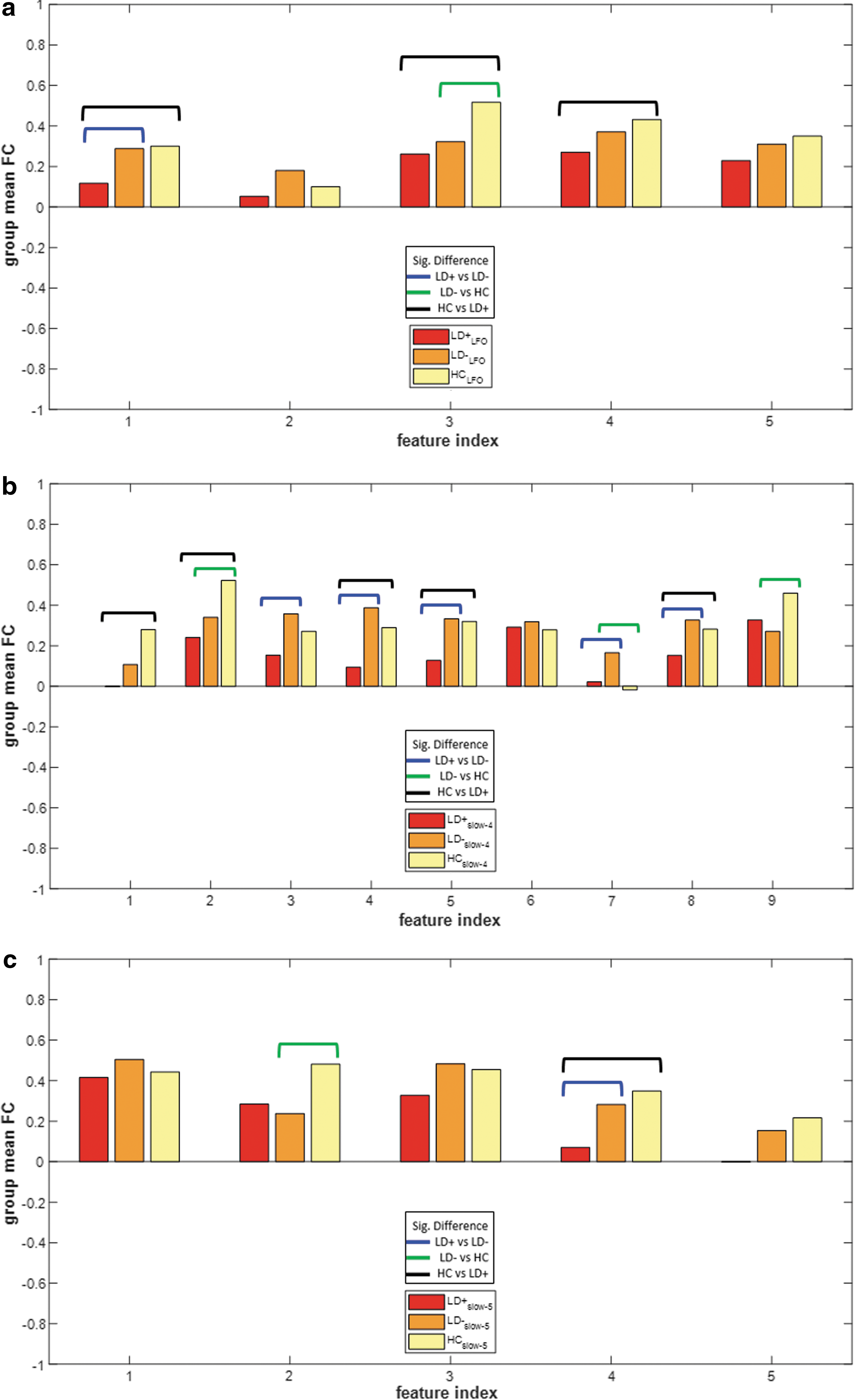
Comparison of mean FC across subgroups LD⁺, LD⁻, and HC involved in classification of left out samples in (a) LFO, (b) slow-4, and (c) slow-5 bands. The individual connections were involved in classifying each left out sample during testing, and the corresponding feature indices can be found in Table 8. The colored lines denote the differences that were significant for p-value <0.05.

In the slow-4 band, the features that were significantly different showed similar gradual increase across some features, as well as comparable mean FC levels between LD⁻ and HC, but significantly different from LD⁺ across other features. No consistent pattern among the mean FC values across subgroups was observed in the slow-5 band. The individual features are listed in Table 8, and features that were significantly different are denoted in Figure 4. The common features across frequency bands are highlighted in Table 8. In particular, connectivity between the right pars opercularis and the left middle frontal seeds was observed to be the only common discriminating feature across all three frequency bands.

Table 8.

Specific Functional Connectivity Features That Discriminate Between Pairs of Subgroups During Classification for the Low Frequency Oscillation, Slow-4, and Slow-5 Bands Arranged in Order of Their Contribution Determined by Support Vector Machine Weights

	LFO		Slow-4		Slow-5
Feature index	ROI 1	ROI 2	ROI 1	ROI 2	ROI 1	ROI 2
1	L Superior temporal	L Inferior temporal	L Superior frontal	Cingulate	L Wernicke	L Inferior temporal
2	R Pars orbitalis	L Inferior temporal	R Pars opercularis	L Middle frontal	R Pars opercularis	L Middle frontal
3	R Pars opercularis	L Middle frontal	R Striate	L Middle frontal	L Ventral thalamus	L Putamen
4	L Ventral thalamus	L Putamen	R Inferior temporal	L Wernicke	R Superior temporal	R Inferior temporal
5	R Pars triangularis	R Inferior temporal	R Striate	L Wernicke	R Superior temporal	R Pars orbitalis
6			R Inferior temporal	R Inferior parietal
7			R Superior temporal	R Pars orbitalis
8			R Striate	R Pars triangularis
9			R Superior temporal	R Striate
Color legend
	Discriminating features common to all frequency bands
	Discriminating features common to slow-4 and slow-5 frequency bands
	Discriminating features common to LFO and slow-5 frequency bands

Common features across subgroups are highlighted as per the color legend above. The feature index corresponds to those depicted in Figure 4.

Discriminating ROIs

Based on the weights assigned to individual features, weights corresponding to individual ROIs were computed by halving weights on FC and assigning to each involved ROI. The weighted ROIs for each classification per frequency band are arranged in order of importance in Table 9 and visualized in Figure 5 using BrainNet Viewer (Xia et al., 2013). From Figure 5, discriminating brain areas common to all three frequency bands involve structures in the frontal brain, namely, the left middle frontal gyrus and the right inferior frontal gyrus (pars opercularis and pars orbitalis). While the frontal and temporal sources appear to show involvement in classification across all three bands, the slow-4 band elicited major contribution from the occipital brain (striate), which could be the reason for a higher classification performance in this band.

FIG. 5.

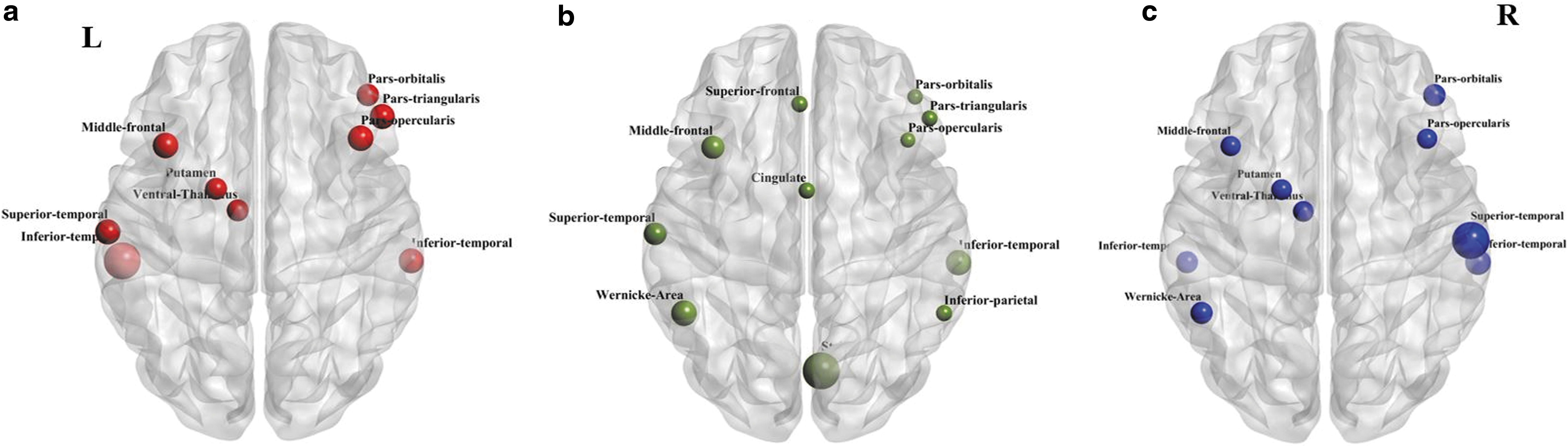
The ROIs involved among the discriminating features corresponding to (a) LFO, (b) slow-4, and (c) slow-5 bands are visualized. The size of the sphere used to represent the ROI is directly proportional to cumulative importance of the ROI.

Table 9.

Weighted Regions of Interest for Each Binary Classifier Per Frequency Band are Listed Below

ROI ID	LFO	Slow-4	Slow-5
1	L Inferior temporal	R Striate	R Superior temporal
2	L Middle frontal	L Wernicke	R Inferior temporal
3	R Pars opercularis	R Inferior temporal	R Pars orbitalis
4	L Superior temporal	L Middle frontal	L Inferior temporal
5	R Inferior temporal	R Superior temporal	L Wernicke
6	R Pars triangularis	Cingulate	L Putamen
7	R Pars orbitalis	L Superior frontal	L Ventral thalamus
8	L Putamen	R Inferior parietal	L Middle frontal
9	L Ventral thalamus	R Pars triangularis	R Pars opercularis
10		R Pars orbitalis
11		R Pars opercularis

The ROIs are arranged in descending order of the weights, that is, ROIs at the top are most important. These ROIs are also visualized by importance in Figure 5.

Main takeaways

Rs-fMRI: a tool for identification of SLD

Results from this study show promise that neuroimaging modality such as rs-fMRI can guide and facilitate the identification of SLD. Unlike neuropsychological assessments that can be time consuming and require active participation from subjects, rs-fMRI requires about 10 min to acquire, is task-free for the subjects, and can expedite the detection SLD in the early-stage poststroke subjects such as in our cohort that might facilitate a speedy recovery and rehabilitation. Whether the same holds true for subclinical deficits arising in nonlanguage domains would require further investigation.

Impact of frequency bands on classification

Comparing the classifier performances across the different frequency bands, it is clear from Table 5 that the FC in the slow-4 band provided the most discriminative power. It was followed by the performances in LFO and slow-5 bands, respectively. This illustrates that FC exhibits multiband property with information distributed over a range of frequencies and limiting the BOLD signal to the LFO could attenuate the effect of individual slow frequency bands. Slow-4 band elicited contributions from occipital brain regions which the other two frequency bands did not. Superior classification based on FC in the slow-4 band might point toward greater amount of disruptions occurring in slow-4 band in comparison to slow-5 band which could reveal more important biomarkers specific to a sample of stroke population such as used in this study.

Machine learning: a tool for automating identification of SLD and understanding group differences

In comparison to a random three-class classifier that is 33.3% accurate, all the three classifiers developed in this study performed reasonably better as per the accuracy levels in Table 5. This demonstrates that machine learning classification can automate the distinction among the LD⁺, LD⁻, and HC. Moreover, such a classification also divulges information about the underlying discriminating features among subgroups. These features are as enumerated in Table 8, and their significance is discussed in further detail in the following section.

Discussion

Overview

Overall, we presented a data-driven approach to differentiate sample stroke subjects with SLD from normal adults. Two types of stroke subgroups were studied, namely, LD⁺, that is, LD⁺ versus those at lower risk of SLD, that is, LD⁻. The results suggested that FC data of the language network can provide relevant information to identify a given subject as belonging to one of the three subgroups, and this might potentially serve as an expedited alternative or supplement to administering the complete detailed battery of neuropsychological assessment. To this end, we automated the classification using multiclass SVM classifier of high performance and identified relevant features and their distribution across the subgroups. Moreover, we analyzed the contribution of FC across slow-4 and slow-5 frequency bands, compared to LFO band, and found that slow-4 offered a better discrimination power in categorizing subjects.

Classification with machine learning

While most studies of the population discrimination based on machine learning apply binary classifiers (Baliki et al., 2011; Chen et al., 2016; Vergun et al., 2013; Wee et al., 2012), we exploited the property of handling more than two classes using multiclass SVM. This not only allowed for comparison between sample stroke and healthy population but also comparison of subgroups within the stroke population and interaction among these subgroups.

We were able to understand the relative contribution of the frequency bands toward classification. Among the three frequency bands, the slow-4 band showed the highest discrimination performance with a more balanced distribution of the left-out samples based on the confusion matrix in Table 5. As expected, across several discriminating features, an increasing trend in the strength of FC was observed from LD⁺ to HC, that is, the LD⁺ showed the weakest FC while the HC group showed the strongest FC with intermediate FC in LD⁻. The significant differences revealed that across the three bands and within the language network, frontal and temporal connectivity differentiated stroke (i.e. LD⁺ and LD⁻) from healthy (i.e. HC), whereas occipital connectivity differentiated between the stroke subgroups.

Involved brain regions

We found connectivity associated with structures of the right inferior frontal gyrus (pars opercularis, pars orbitalis, pars triangularis in LFO, slow-4; pars orbitalis and pars opercularis in slow-5) to be discriminatory, which is homologous to the left inferior frontal language areas in right handed subjects. This could be the result of recruitment of the homotopic right cortex due to damage to left language regions in LD⁺ (Blank et al., 2003; Rosen et al., 2000). The other common node found across all bands included the left middle frontal gyrus (BA 46) and demonstrated decreased FC in the stroke (LD⁺ and LD⁻) subgroups relative to the HC subgroup, which could be suggestive of the differences in executive control resulting from stroke (Elliott, 2003). Unique to the slow-4 band was the connectivity associated with the striate (BA 17). Majority of the associated connections exhibited a significant difference between the LD⁺ and LD⁻ subgroups but no significant difference between the LD⁻ and HC subgroups. Underengagement in this posterior cortical system could be indicative of deficit in phonological processing in LD⁺ (Pugh et al., 2000; Shaywitz et al., 2001). Congruence of our results with prior research suggests biological plausibility of the features selected by NCA for classification.

Slow-4 dependence of FC

On one hand, numerous studies have reported relevance of rs-fMRI connectivity measures derived from the slow-4 band. Amplitude fluctuations in slow-4 have proven to offer greater test-retest reliability in a cohort of healthy adults (Zuo et al., 2010). Specifically, Zuo et al. (2010) also pointed at robustness in slow-4 band in brain regions, including basal ganglia, which has been shown to be an important center in the language network of the brain (Booth et al., 2007). Slow-4 has also been demonstrated to be important in finding abnormalities in Schizophrenia in regions and linked with reduced FC in lingual gyrus (Hoptman et al., 2010). Furthermore, slow-4 has been capable of offering superior diagnostic information in case of autism, which is primarily associated with language abnormalities, in children (Di Martino et al., 2008) and adolescents (Chen et al., 2016). The boosted classification using FC in the slow-4 band with a focus on the language network puts findings from our study in alignment with the aforementioned studies.

Slow-5 dependence of FC

On the other hand, there is strong evidence of connectivity in slow-5 band being important as well. Previous studies from our laboratory have demonstrated FC in the slow-5 band to be a marker of stroke recovery (La et al., 2016a,b). Regional and network level FC metrics were found to be more relevant in the healthy brain specific to sensorimotor structures (Xue et al., 2014). The potential of FC in the slow-5 band as a biomarker in other neurological and psychiatric disorders have also been reported. For example, in subjects with mild cognitive impairment, amplitude based FC was greater in the slow-5 band concentrated in the occipital regions of the brain (Han et al., 2011). Topographical changes in fMRI revealed significant information in the sensorimotor and default mode networks in subjects with bipolar disorder and mania (Martino et al., 2016). Greater performance in differentiation using SVM between a vascular dementia group relative to a HC group was illustrated in the slow-5 band (Zhang et al., 2013).

Frequency dependence of FC

In agreement with the studies described above and others (Gohel and Biswal, 2015), our findings reveal that contribution of neuronal information, as measured by BOLD signals, is different across frequency bands in our sample study cohort. While this effect has been observed in sample groups from different populations as described above, our study adds to the literature for the stroke population based on FC from a representative cohort. Our results could imply that disruptions in brain due to stroke are more pronounced in slow-4 than in slow-5 and combining them into the whole band might be diminishing the effects of individual slow bands. Amplitude-based (non-FC) metric has been known to exhibit reduced connectivity in posterior parts of default mode network in stroke subjects (La et al., 2016b).

A possible ramification of varying information across frequency bands could be that BOLD signal might be sensitive to different frequency bands based on the population, that is, connectivity in the slow-4 band might play a dominant role for the stroke subgroups (LD⁺ and LD⁻). However, the LFO band also was equally indicative in differentiating the HC subgroup. This could imply that slow-4 oscillations could be better indicative of the early stages of stroke in comparison to LFO found in healthy subjects. From the findings of the current study, language regions in the occipital brain appeared to be relatively more involved and sensitive in the slow-4 band, while language areas of the frontal and temporal brain seemed sensitive in the slow-5 and LFO bands. A comprehensive and comparative analysis of FC from major brain networks would be required to confirm this in other brain networks.

Limitations

Our study was constrained in terms of the sample size since conventional machine learning analysis is built upon training on a large dataset so as to have greater power of generalizability. While the accuracy levels obtained from the nested cross-validation were reasonably better than random chance levels, the performance could be further boosted with a larger sample size. Thus, results from this study should not be used to draw conclusions about the stroke population in general. However, this study showed that machine learning has the potential to automate the system of identification of SLD, given a wide variety of brain profiles.

We constructed the resting-state FC within the language network using the seed regions provided (Tomasi and Volkow, 2012). While this template covers crucial regions of the language network, multiple studies have located varying coordinates for the same (Ferstl et al., 2008; Saur et al., 2008). In addition, to evaluate FC, we used interregional Pearson's correlation coefficients, which is a classical approach. However, recent studies (Smith et al., 2011) provide alternate definitions of FC such as mutual information, cosine similarity, dynamic time warping, and so on. Using different definitions of seeds and FC could influence the selected features in the FC pattern classification.

There could be several confounding factors while studying brain differences in population groups. We eliminated potential confounding effects by limiting the analysis to right-handed subjects who were matched by age, gender, and education. Effects of subclinical deficits may have long-term impact on subject's life as time since stroke increases. It is potentially easier to detect deficits at the earliest after the stroke to pursue adequate management to have better patient outcomes. To avoid variability of time since stroke onset, stroke subjects in the early-stage (within 30 days of stroke onset) only were included in this analysis. Although stroke severity could be considered a surrogate for lesion volume in stroke subjects, the impact could not be studied due to missing data for a few subjects.

The ongoing recruitment of this study offers future scope to incorporate more subjects that can form a more homogenous cohort and even expand the analysis to subclinical deficits in the nonlanguage networks of the brain. Findings from our study are in alignment with several works in literature and draw attention to investigation of population with subclinical deficits which could often be overlooked.

Conclusion

We utilized SVM classifier to discriminate sample LD⁺ from LD⁻ from healthy normal subjects using FC in the language network derived from three frequency bands. This analysis points to the following conclusions: (1) FC derived from a 10-min rs-fMRI has the potential to identify whether a given subject is at risk of having SLD poststroke; (2) resting-state FC corresponding to the slow-4 frequency band offers better classification performance in comparison to that from slow-5 or LFO bands, thus, suggesting that slow-4 reflects more relevant FC; and (3) using a multiclass machine learning SVM classifier facilitates automated identification of SLD as validated by the LOOCV accuracy from nested cross-validation. These outcomes imply the possibility of using such an automated methodology in conjunction with or as a surrogate to neuropsychological assessment for easier and accelerated identification of SLD.

Footnotes

Acknowledgments

The authors extend thanks to all the study subjects and their families for participation and MR technologists for acquiring imaging data. This work was supported by NIH grants RC1MH090912-01, T32GM008692, UL1TR000427, K23NS086852, T32EB011434, R01EB000856-06, and R01EB009103-01 and by the DARPA RCI Program (MTO) N66001-12-C-4025 and HIST Program (MTO) N66001-11-1-4013. Additional funding was also provided through the AHA Grant 1T32EB011434-01A1, AHA Innovative Research Award–National (Marcus Foundation) 15IRG22760009, AHA Midwest Grant in Aid Award 15GRNT25780033, the Foundation of ASNR, UW Milwaukee-Madison Intercampus Grants, the UW Graduate School, and by Shapiro Foundation Grants.

Author Disclosure Statement

No competing financial interests exist.

References

Allwein

, Schapire

, Singer

. 2000. Reducing multiclass to binary: a unifying approach for margin classifiers. J Mach Learn Res, 1:113–141.

Baliki

, Baria

, Apkarian

. 2011. The cortical rhythms of chronic back pain. J Neurosci, 31:13981–13990.

Biswal

, Zerrin Yetkin

, Haughton

, Hyde

. 1995. Functional connectivity in the motor cortex of resting human brain using echo-planar MRI. Magn Reson Med, 34:537–541.

Blank

, Bird

, Turkheimer

, Wise

. 2003. Speech production after stroke: the role of the right pars opercularis. Ann Neurol, 54:310–320.

Booth

, Wood

, Lu

, Houk

, Bitan

. 2007. The role of the basal ganglia and cerebellum in language processing. Brain Res, 1133:136–144.

Buzsáki

, Draguhn

. 2004. Neuronal oscillations in cortical networks. Science, 304:1926–1929.

Cawley

, Talbot

. 2010. On over-fitting in model selection and subsequent selection bias in performance evaluation. J Mach Learn Res, 11:2079–2107.

Chen

, Duan

, Liu

, et al. 2016. Multivariate classification of autism spectrum disorder using frequency-specific resting-state functional connectivity—a multi-center study. Prog Neuropsychopharmacol Biol Psychiatry, 64:1–9.

Cortes

, Vapnik

. 1995. Support-vector networks. Mach Learn, 20:273–297.

10.

Cox

. 1996. AFNI: software for analysis and visualization of functional magnetic resonance neuroimages. Comput Biomed Res, 29:162–173.

11.

Cox

, Jesmanowicz

. 1999. Real-time 3D image registration for functional MRI. Magn Reson Med, 42:1014–1018.

12.

Demirhan

, Nir

, Zavaliangos-Petropulu

, et al. 2015. Feature selection improves the accuracy of classifying alzheimer disease using diffusion tensor images. Proc IEEE Int Symp Biomed Imaging, 2015:126–130.

13.

Dickerson

, Salat

, Greve

, et al. 2005. Increased hippocampal activation in mild cognitive impairment compared to normal aging and AD. Neurology, 65:404–411.

14.

Di Martino

, Ghaffari

, Curchack

, et al. 2008. Decomposing intra-subject variability in children with attention-deficit/hyperactivity disorder. Biol Psychiatry, 64:607–614.

15.

Dosenbach

, Nardos

, Cohen

, et al. 2010. Prediction of individual brain maturity using fMRI. Science, 329:1358–1361.

16.

Elliott

. 2003. Executive functions and their disorders: imaging in clinical neuroscience. Br Med Bull, 65:49–59.

17.

Ferstl

, Neumann

, Bogler

, Von Cramon

. 2008. The extended language network: a meta-analysis of neuroimaging studies on text comprehension. Hum Brain Mapp, 29:581–593.

18.

Friston

, Ashburner

, Frith

, Poline

, Heather

, Frackowiak

. 1995. Spatial registration and normalization of images. Hum Brain Mapp, 3:165–189.

19.

Gohel

, Biswal

. 2015. Functional integration between brain regions at rest occurs in multiple-frequency bands. Brain Connect, 5:23–34.

20.

Goldberger

, Hinton

, Roweis

, Salakhutdinov

. 2005. Neighbourhood components analysis. Adv Neural Inf Process Syst, 2005:513–520.

21.

Hämäläinen

, Pihlajamäki

, Tanila

, et al. 2007. Increased fMRI responses during encoding in mild cognitive impairment. Neurobiol Aging, 28:1889–1903.

22.

Han

, Wang

, Zhao

, et al. 2011. Frequency-dependent changes in the amplitude of low-frequency fluctuations in amnestic mild cognitive impairment: a resting-state fMRI study. Neuroimage, 55:287–295.

23.

Hastie

, Tibshirani

, Friedman

. 2001. The Elements of Statistical Learning. New York, NY: Springer.

24.

Hommel

, Miguel

, Naegele

, Gonnet

, Jaillard

. 2009. Cognitive determinants of social functioning after a first ever mild to moderate stroke at vocational age. J Neurol Neurosurg Psychiatry, 80:876–880.

25.

Hoptman

, Zuo

X-N

, Butler

, Javitt

, D'Angelo

, Mauro

, Milham

. 2010. Amplitude of low-frequency oscillations in schizophrenia: a resting state fMRI study. Schizophr Res, 117:13–20.

26.

Hwang

, Nair

, Mathis

, Cook

, Mohanty

, Zhao

, et al. 2019. Using low-frequency oscillations to detect temporal lobe epilepsy with machine learning. Brain Connect, 9:185–194.

27.

Ivnik

, Malec

, Smith

, Tangalos

, Petersen

. 1996. Neuropsychological tests' norms above age 55: COWAT, BNT, MAE token, WRAT-R reading, AMNART, STROOP, TMT, and JLO. Clin Neuropsychol, 10:262–278.

28.

Knecht

, Deppe

, Dräger

, Bobe

, Lohmann

, Ringelstein

E-B

, Henningsen

. 2000. Language lateralization in healthy right-handers. Brain, 123:74–81.

29.

Knerr

, Personnaz

, Dreyfus

. 1990. Single-layer learning revisited: a stepwise procedure for building and training a neural network. In: Soulié

, Hérault

(eds.) Neurocomputing: Algorithms, Architectures and Applications, vol 68. Berlin, Heidelberg: Springer; p. 71.

30.

, Mossahebi

, Nair

, et al. 2016a. Differing patterns of altered slow-5 oscillations in healthy aging and ischemic stroke. Front Hum Neurosci, 10:156.

31.

, Nair

, Mossahebi

, et al. 2016b. Implication of the Slow-5 oscillations in the disruption of the default-mode network in healthy aging and stroke. Brain Connect, 6:482–495.

32.

Leys

, Ley

, Klein

, Bernard

, Licata

. 2013. Detecting outliers: do not use standard deviation around the mean, use absolute deviation around the median. J Exp Soc Psychol, 49:764–766.

33.

Martino

, Magioncalda

, Huang

, et al. 2016. Contrasting variability patterns in the default mode and sensorimotor networks balance in bipolar depression and mania. Proc Natl Acad Sci USA, 113:4824–4829.

34.

Meier

, Desphande

, Vergun

, et al. 2012. Support vector machine classification and characterization of age-related reorganization of functional brain networks. Neuroimage, 60:601–613.

35.

Mitchell

, Kemp

, Benito-León

, Reuber

. 2010. The influence of cognitive impairment on health-related quality of life in neurological disease. Acta Neuropsychiatrica, 22:2–13.

36.

Mohanty

, Nair

, Tellapragada

, Advani

, Williams

Jr , Prabhakaran

. 2018. Abstract WP141: prediction of subclinical language deficit using machine learning based on post-stroke functional connectivity derived from low frequency oscillations. Stroke, 49:AWP141.

37.

Mohanty

, Sinha

, Remsik

, et al. 2018. Machine learning classification to identify the stage of brain-computer interface therapy for stroke rehabilitation using functional connectivity. Front Neurosci, 12:353.

38.

Murphy

, Fox

. 2016. Towards a consensus regarding global signal regression for resting state functional connectivity MRI. Neuroimage, 154:169–173.

39.

Nair

, Young

, La

, et al. 2015. Functional connectivity changes in the language network during stroke recovery. Ann Clin Transl Neurol, 2:185–195.

40.

Nys

, Van Zandvoort

, De Kort

, Jansen

, Van der Worp

, Kappelle

, De Haan

. 2005. Domain-specific cognitive recovery after first-ever stroke: a follow-up study of 111 cases. J Int Neuropsychol Soc, 11:795–806.

41.

Ochsner

, Bunge

, Gross

, Gabrieli

. 2002. Rethinking feelings: an FMRI study of the cognitive regulation of emotion. J Cogn Neurosci, 14:1215–1229.

42.

Patterson

. 2011. Controlled oral word association test. In: Kreutzer

, DeLuca

, Caplan

(eds.) Encyclopedia of Clinical Neuropsychology. New York, NY: Springer; p. 703–706.

43.

Penttonen

, Buzsáki

. 2003. Natural logarithmic relationship between brain oscillators. Thalamus Relat Syst, 2:145–152.

44.

Power

, Barnes

, Snyder

, Schlaggar

, Petersen

. 2012. Spurious but systematic correlations in functional connectivity MRI networks arise from subject motion. Neuroimage, 59:2142–2154.

45.

Pugh

, Mencl

, Shaywitz

, et al. 2000. The angular gyrus in developmental dyslexia: task-specific differences in functional connectivity within posterior cortex. Psychol Sci, 11:51–56.

46.

Rombouts

, Barkhof

, Goekoop

, Stam

, Scheltens

. 2005. Altered resting state networks in mild cognitive impairment and mild Alzheimer's disease: an fMRI study. Hum Brain Mapp, 26:231–239.

47.

Rosen

, Petersen

, Linenweber

, et al. 2000. Neural correlates of recovery from aphasia after damage to left inferior frontal cortex. Neurology, 55:1883–1894.

48.

Rosso

, Valabregue

, Attal

, et al. 2013. Contribution of corticospinal tract and functional connectivity in hand motor impairment after stroke. PLoS One, 8:e73164.

49.

Ruff

, Light

, Parker

, Levin

. 1996. Benton controlled oral word association test: reliability and updated norms. Arch Clin Neuropsychol, 11:329–338.

50.

Saur

, Kreher

, Schnell

, et al. 2008. Ventral and dorsal pathways for language. Proc Natl Acad Sci USA, 105:18035–18040.

51.

Schaechter

. 2004. Motor rehabilitation and brain plasticity after hemiparetic stroke. Prog Neurobiol, 73:61–72.

52.

Shaywitz

, Shaywitz

, Pugh

, et al. 2001. The neurobiology of dyslexia. Clin Neurosci Res, 1:291–299.

53.

Smith

, Miller

, Salimi-Khorshidi

, et al. 2011. Network modelling methods for FMRI. Neuroimage, 54:875–891.

54.

Smyser

, Inder

, Shimony

, Hill

, Degnan

, Snyder

, Neil

. 2010. Longitudinal analysis of neural network development in preterm infants. Cereb Cortex, 20:2852–2862.

55.

Snoek

, Larochelle

, Adams

. 2012. Practical bayesian optimization of machine learning algorithms. Adv Neural Inf Process Syst, 2012:2951–2959.

56.

Stephens

, Kenny

, Rowan

, et al. 2005. Association between mild vascular cognitive impairment and impaired activities of daily living in older stroke survivors without dementia. J Am Geriatr Soc, 53:103–107.

57.

Szaflarski

, Vannest

, Wu

, DiFrancesco

, Banks

, Gilbert

. 2011. Excitatory repetitive transcranial magnetic stimulation induces improvements in chronic post-stroke aphasia. Med Sci Mon, 17:CR132.

58.

Tang

, Zhao

, Chen

, et al. 2016. Decreased functional connectivity of homotopic brain regions in chronic stroke patients: a resting state fMRI study. PLoS One, 11:e0152875.

59.

Tomasi

, Volkow

. 2012. Resting functional connectivity of language networks: characterization and reproducibility. Mol Psychiatry, 17:841–854.

60.

Tombaugh

, Kozak

, Rees

. 1999. Normative data stratified by age and education for two measures of verbal fluency: FAS and animal naming. Arch Clin Neuropsychol, 14:167–177.

61.

Van Dijk

, Sabuncu

, Buckner

. 2012. The influence of head motion on intrinsic functional connectivity MRI. Neuroimage, 59:431–438.

62.

Vergun

, Deshpande

, Meier

, et al. 2013. Characterizing functional connectivity differences in aging adults using machine learning on resting state fMRI data. Front Comput Neurosci, 7:38.

63.

Ward

, Brown

, Thompson

, Frackowiak

. 2003. Neural correlates of motor recovery after stroke: a longitudinal fMRI study. Brain, 126:2476–2496.

64.

Wee

C-Y

, Yap

, Denny

, et al. 2012. Resting-state multi-spectrum functional connectivity networks for identification of MCI patients. PLoS One, 7:e37828.

65.

Xia

, Wang

, He

. 2013. BrainNet Viewer: a network visualization tool for human brain connectomics. PLoS One, 8:e68910.

66.

Xue

S-W

, Li

, Weng

X-C

, Northoff

, Li

D-W

. 2014. Different neural manifestations of two slow frequency bands in resting functional magnetic resonance imaging: a systemic survey at regional, interregional, and network levels. Brain Connect, 4:242–255.

67.

Yang

, Wang

, Zuo

. 2012. Neighborhood component feature selection for high-dimensional data. JCP, 7:161–168.

68.

Zhang

, Liu

, Chen

, Peng

, Liu

, Fan

, et al. 2013. Determination of vascular dementia brain in distinct frequency bands with whole brain functional connectivity patterns. PLoS One, 8:e54512.

69.

Zuo

X-N

, Di Martino

, Kelly

, et al. 2010. The oscillating brain: complex and reliable. Neuroimage, 49:1432–1445.