Comparison of Methods to Identify Modules in Noisy or Incomplete Brain Networks

Abstract

Community structure, or “modularity,” is a fundamentally important aspect in the organization of structural and functional brain networks, but their identification with community detection methods is confounded by noisy or missing connections. Although several methods have been used to account for missing data, the performance of these methods has not been compared quantitatively so far. In this study, we compared four different approaches to account for missing connections when identifying modules in binary and weighted networks using both Louvain and Infomap community detection algorithms. The four methods are “zeros,” “row-column mean,” “common neighbors,” and “consensus clustering.” Using Lancichinetti–Fortunato–Radicchi benchmark-simulated binary and weighted networks, we find that “zeros,” “row-column mean,” and “common neighbors” approaches perform well with both Louvain and Infomap, whereas “consensus clustering” performs well with Louvain but not Infomap. A similar pattern of results was observed with empirical networks from stereotactical electroencephalography data, except that “consensus clustering” outperforms other approaches on weighted networks with Louvain. Based on these results, we recommend any of the four methods when using Louvain on binary networks, whereas “consensus clustering” is superior with Louvain clustering of weighted networks. When using Infomap, “zeros” or “common neighbors” should be used for both binary and weighted networks. These findings provide a basis to accounting for noisy or missing connections when identifying modules in brain networks.

Introduction

The topological organization of interregional human brain networks can reveal how different parts of the brain interact to produce cognition and behavior (van den Heuvel and Sporns, 2013). Several studies have mapped structural connections between regions using diffusion magnetic resonance imaging (MRI; Catani and de Schotten, 2012; Schmahmann and Pandya, 2009) and functional connections using electroencephalography (EEG)/magnetoencephalography (MEG; de Haan et al., 2009; Stam et al., 2008), and functional magnetic resonance imaging (fMRI; Buckner and Vincent, 2007; Salvador et al., 2005). The resulting brain networks are typically characterized with mathematical tools and concepts from graph theory (Bullmore and Sporns, 2009) in many of these studies.

In particular, a number of studies have used community detection methods from graph theory to identify modules, that is, sets of densely interconnected nodes, in interregional human structural (Hagmann et al., 2008), and functional networks (Chavez et al., 2010; Nicolini and Bifone, 2016; Power et al., 2011).

Modules constitute organizational units of the network (Sporns and Betzel, 2016) and may have distinct functional roles (Wig, 2017). Modules identified in structural brain networks of both humans (Hagmann et al., 2008) and animals (Bota et al., 2015; Harriger et al., 2012; Wang et al., 2012) follow known functional subdivisions in the brain, that is, modules comprise regions that are known to be functionally related from previous lesion and imaging studies. Also the modules identified in functional brain networks obtained from fMRI resting-state data (Power et al., 2011) correspond to functional systems of the brain previously identified by other techniques such as independent component analysis (Beckmann et al., 2005; Damoiseaux et al., 2006).

However, structural and functional networks obtained with noninvasive methodologies contain a number of connections that are noisy, difficult to estimate, or are significantly biased by various factors. In MEG/EEG, the low signal-to-noise ratio and field spread/volume conduction pose problems in identifying functional connections, especially between nearby brain regions (Hillebrand et al., 2012; Palva and Palva, 2012; Palva et al., 2018). Also in fMRI, short-range correlations between voxels are artificially high due to effects of local vasculature, preprocessing, and motion artifacts (Power et al., 2011). Similarly, with diffusion MRI, some structural connections cannot be accurately identified due to technical factors (e.g., subject motion and physiological noise) or algorithmic confounds caused by crossing fibers (Dell'Acqua et al., 2007; Thomas et al., 2014).

Moreover, interregional functional networks derived from invasive human electrophysiological techniques such as stereotactical EEG (SEEG) and electrocorticography (ECoG) inherently yield only a sparse sampling of brain areas (Arnulfo et al., 2015a; Zhang et al., 2010). Hence, both noninvasive (MEG, EEG, fMRI, and diffusion MRI) and invasive (SEEG and ECoG) connectomes are invariably derived from data with incomplete coverage and thus a number of missing connections between brain regions.

Modules are often identified using various community detection methods. Community detection methods such as Louvain (Blondel et al., 2008) and Infomap (Rosvall and Bergstrom, 2008) can, however, be confounded when the network contains noisy connections as in MEG/EEG, diffusion MRI, or fMRI, or missing connections as in SEEG or ECoG. For example, when signal between neighboring voxels in fMRI are artificially correlated, modules identified from voxel-wise functional networks would be biased toward comprising spatially contiguous voxels.

One way of accounting for noisy connections has been to set all these connections to 0 before identifying modules (Power et al., 2011). However, this makes strong assumptions about the underlying connections, which could itself bias the identification of modules, especially when the proportion of noisy connections is high. Although this is the only method to our knowledge that has been employed to identify modules in noisy or incomplete brain networks, a number of general “link prediction” methods from network science have been used to replace noisy or missing connections to generate complete networks (Lü and Zhou, 2011).

One of the most widely used link prediction methods is the “common neighbors” approach, which inserts connections between nodes that are similar to each other, where similarity is quantified by correspondence of local neighborhoods (Goldberg and Roth, 2003). Other similarity-based link prediction methods such as the Local Path Index (Lü et al., 2009) use quasi-local topological information to quantify similarity between pairs of nodes, whereas yet others such as SimRank (Jeh and Widom, 2002) use global topological organization to quantify similarity.

Conversely, model-based link prediction methods fit a specific generative network model to the original network and use the estimated model parameters to generate complete networks. Examples are methods based on stochastic relational models (Yu et al., 2006), hierarchical structure models (Clauset et al., 2008), or stochastic block models (Airoldi et al., 2008; Dorelan et al., 2005). Therefore, a range of methods exist to replace noisy or missing connections in incomplete networks, but there has not yet been a systematic comparison of these methods or their ability to facilitate the accurate identification of modules in brain networks.

In this article, we compared the performance of four possible methods to account for noisy or missing values when identifying modules in brain networks. The four methods represent distinct approaches to filling noisy or missing connections to yield complete networks. The first method is to set noisy or missing values to 0, whereas the second method is to replace each of these connections by the mean of the respective row and column elements. A third method is to replace each noisy or missing connection by its proportion of common neighbors (Goldberg and Roth, 2003), whereas a fourth method uses consensus clustering approaches (Lancichinetti and Fortunato, 2012) to identify modules.

We compared the performance of these methods on incomplete versions of binary and weighted Lancichinetti–Fortunato–Radicchi (LFR) benchmark simulated networks (Lancichinetti et al., 2008), with both Louvain and Infomap community detection algorithms. We also compared the performance of these methods with Louvain and Infomap, on binary and weighted versions of an incomplete group-level functional connectome obtained from SEEG data of 64 individuals.

We show on simulated networks that each of the four methods can be used with the Louvain community detection algorithm to identify modules with high accuracy, despite a substantial percentage of missing connections. When used with Infomap, however, the “zeros,” “row-column mean,” and “common neighbors” approaches perform well, whereas the “consensus clustering” approach identifies modules less accurately when a substantial percentage of connections are missing. Furthermore, we demonstrate on empirical SEEG networks that the “consensus clustering” approach outperforms the other methods when using Louvain with weighted networks, whereas the “zeros” or “common neighbors” methods perform well when Infomap is used to identify modules.

In the following sections, we describe comparisons of these four approaches to identify modules in brain networks with missing connections. However, the methods compared can be applied in an identical manner to brain networks with noisy connections, and the results obtained are equally relevant to identifying modules in brain networks with noisy connections.

Materials and Methods

Description of methods to account for missing connections

We compared four methods to identify modules in incomplete brain networks:

Zeros: In this method, each missing value is replaced by 0 before identifying modules in the network. This was done for both binary and weighted networks.

Row-column mean: In this method, each missing value is replaced by mean of a vector containing all valid row and column elements of that missing value. This generates complete networks while making minimal assumptions about underlying connections. For binary networks, the element is set to 1 if the vector mean is ≥0.5, otherwise it is set to 0. For weighted networks, the connection weight is set to the vector mean. The complete matrix is entered into the method for identifying modules.

Common neighbors: In this method, each missing value is replaced by the proportion of neighbors that are common to both nodes between which the missing value exists. This method represents a well-known approach to link prediction in complex networks (Goldberg and Roth, 2003; Lü and Zhou, 2011), and notably, it corresponds to a known principle of brain network organization (Vértes et al., 2012). The measure is also called the Jaccard coefficient (Jaccard, 1912). For binary networks, the element is set to 1 when the proportion is ≥0.5, otherwise it is set to 0. For weighted networks, the connection weight is set to the proportion of common neighbors. When either node has no connections, the matrix element is set to 0. The complete matrix is entered into the method for identifying modules.

Consensus clustering: In this method, missing values are replaced by randomly selecting existing values from the network (with replacement). This process is repeated 100 times to generate an ensemble of complete networks. Modules are identified on each of these complete networks and the partitions of nodes into modules for each of these networks are then combined using a consensus clustering approach. Although consensus clustering (Lancichinetti and Fortunato, 2012) has been used to identify modules in networks, we use it here for the first time to identify modules in incomplete brain networks.

To combine the 100 individual partitions into a consensus partition, each partition is represented as a binary square matrix, where each element is set to 1 or 0 depending, respectively, on whether those pairs of nodes are in the same module or not. This makes the partitions comparable with each other, since the arbitrary numbering of modules is eliminated in the representation. The ensemble of matrices is then averaged (along the dimension of the repetitions) to obtain a consensus matrix with values close to 1 when the respective pair of nodes frequently co-occurred in the same module across the ensemble and values close to 0 when the respective pair of nodes rarely co-occurred in the same module across the ensemble.

For binary networks, all values ≥0.5 in this consensus matrix or network are set to 1, whereas all other values are set to 0. For weighted networks, the consensus matrix with values from 0 to 1 is used. The binary or weighted network is entered into the method for identifying modules.

Community detection methods used

We compared the performance of the mentioned four methods to identify modules in incomplete brain networks, with two community detection algorithms Louvain and Infomap, which have been widely used in brain imaging studies (Betzel et al., 2016; Meunier et al., 2009; Nicolini et al., 2017; Power et al., 2011). The “gamma” parameter for Louvain method, which influences the number of modules obtained, was set to 1. We used the implementation of the Louvain method available in the Brain Connectivity Toolbox (Rubinov and Sporns, 2010).

For Infomap, network density, that is, the number of connections as a percentage of the total possible number of connections, influences the number of modules. This can cause problems after the first stage of “consensus clustering,” which yields a densely connected consensus matrix. In such cases, only values in the top 10 percentile of the consensus matrix were retained, hence network density was set to 10%. We used the implementation of the Infomap method from the Map Equation website (www.mapequation.org).

The parameter settings for each of the four methods, when used in combination with Louvain and Infomap algorithms, are tabulated (Table 1).

Table 1.

Parameter Settings for Each of Four Methods to Account for Missing Connections

	Zeros	Row-column mean	Common neighbors	Consensus clustering
Louvain
Binary
Gamma	1	1	1	1
Threshold	N/A	0.5	0.5	0.5
Replicates	N/A	N/A	N/A	100
Weighted
Gamma	1	1	1	1
Replicates	N/A	N/A	N/A	100
Infomap
Binary
Network density	10%	10%	10%	10%
Threshold	N/A	0.5	0.5	0.5
Replicates	N/A	N/A	N/A	100
Weighted
Network density	10%	10%	10%	10%
Replicates	N/A	N/A	N/A	100

Parameter settings for each of four methods as applied with Louvain and Infomap algorithms to both binary and weighted networks. The “gamma” value is the resolution parameter that influences the number of modules with Louvain, whereas “network density” plays the corresponding function with Infomap. The “threshold” value is used for binary networks with both Louvain and Infomap. Connections below the “threshold” value are set to 0, whereas those above the “threshold” are set to 1. The “replicates” parameter is used only with “consensus clustering,” and indicates the number of randomly filled versions of the original network, from which consensus modules are identified. The network density of 10% was imposed on the consensus matrix during “consensus clustering” for both simulated and empirical networks. However, network density of 10% for the original input networks for each of the four methods was imposed only on the empirical networks.

N/A, not applicable.

MATLAB code for each of the four methods to account for missing connections in binary and weighted networks, with both Louvain and Infomap algorithms, has been made available at (https://github.com/nitinwilliams/eeg_meg_analysis/tree/master/missingvalues_toolbox).

Simulations on LFR benchmark networks

To assess performance of the four different methods, we generated LFR benchmark networks (Lancichinetti et al., 2008) that have been used to compare different community detection algorithms (Lancichinetti and Fortunato, 2009b). These networks mimic real-world networks since their degree distribution and distribution of module sizes follow power law distributions.

We used open source code (https://sites.google.com/site/andrealancichinetti/files) to generate LFR binary and weighted undirected networks with 74 nodes, representing brain regions from a single hemisphere as per Destrieux brain parcellation (Destrieux et al., 2010). The settings to generate the binary networks were such that mean degree was 10, maximum degree was 20, whereas minimum and maximum community sizes were set to 6 and 12, respectively. To mimic values found in real-world networks, we chose 2 and 1 as the power law exponents for degree distribution and distribution of communities, respectively (Lancichinetti et al., 2008).

With these parameters, we generated networks at mixing factors from 0.05 to 0.4 (intervals of 0.05)—mixing factor indicates the distinctness of modules from each other and is a parameter that can be set in generating LFR networks. Low values for mixing factors produce networks with highly distinct modules. A single network was generated for each level of mixing factor such that eight LFR benchmark networks were obtained and the ground truth community structure for each of these networks was also recorded. We followed an identical procedure to generate weighted networks, except that strengths of within module and between module connections were sampled from normal distributions with mean 0.7 and 0.3, respectively, each distribution with standard deviation (SD) of 0.1. All connection strengths were constrained to be positive.

From each of these binary and weighted networks, we created ensembles of incomplete networks by randomly replacing a proportion of existing values by NaN (not-a-number), to indicate invalid entries. Specifically, we created 100 incomplete networks each, at 9 levels of “proportion of missing values” ranging from 0.1 to 0.9 (intervals of 0.1). Proportion of missing values of 0.9 meant that 90% of existing values were replaced by NaN values. This was done for each of the original eight networks (each with different mixing factors). Thus, 100 incomplete versions of each of the 8 binary and weighted networks were created at 9 levels of “proportion of missing values.”

To each of these networks, we applied both Louvain and Infomap algorithms to identify modules, using each of the four ways of accounting for missing connections. For each of the networks, the identified modules were compared with the ground truth modules using a measure of partition similarity: \documentclass{aastex}\usepackage{amsbsy}\usepackage{amsfonts}\usepackage{amssymb}\usepackage{bm}\usepackage{mathrsfs}\usepackage{pifont}\usepackage{stmaryrd}\usepackage{textcomp}\usepackage{portland, xspace}\usepackage{amsmath, amsxtra}\usepackage{upgreek}\pagestyle{empty}\DeclareMathSizes{10}{9}{7}{6}\begin{document} \begin{align*} PS \;= \; { \frac { \left\langle { l1 , l2 } \right\rangle } { \sqrt { \left\langle { l1 , l1 } \right\rangle \left\langle { l2 , l2 } \right\rangle } } } , \end{align*} \end{document}

which gives values between 0 and 1 (1 being identical partitions). To assess performance of the methods to account for missing values, we inspected mean partition similarity across 100 incomplete networks (compared with ground truth partitions), for each combination of “mixing factor” and “proportion of missing values.”

In addition to comparing similarity between estimated and ground truth modules across the four methods, we also compared computation times of these approaches. Louvain algorithm was run on Intel (R) Xeon (R) X5680 processor, with speed 3.33 GHz. Infomap algorithm was run on Intel (R) Xeon (R) E560 processor, with speed 2.40 GHz.

To assess performance and computation time for larger networks, we also compared the four methods on single examples of 10³ node LFR binary and weighted networks, across the range of mixing factors, for proportions of missing values of 0.3, 0.5, and 0.7. The parameters to generate these networks were the same as for the original 74 node networks, except that mean degree, maximum degree, and minimum and maximum community sizes were linearly scaled to the 10³ node setting, with values of 135, 270, 81, and 162, respectively.

Investigations on group-level functional connectome from SEEG resting-state data

Data acquisition and preprocessing

We recorded 10 minutes eyes-closed resting-state SEEG data at 1 kHz, from 64 individuals affected by drug-resistant focal epilepsy and undergoing presurgical clinical assessment. For each individual, 17 ± 3 (mean ± SD) SEEG shafts were inserted into the brain, with anatomical positions varying by surgical requirements (Cardinale et al., 2013). The study was approved by ethics committee of the Niguarda “Ca’ Granda” Hospital, Milan, and done as per World Medical Association Declaration of Helsinki—Ethical Principles for Medical Research Involving Human Subjects.

After rereferencing each gray matter contact to its nearest white matter contact (Arnulfo et al., 2015a), data were finite impulse response filtered into 18 frequency bands from 3 to 320 Hz, out of which only activity from the alpha frequency band of 8–12 Hz (center frequency = 10 Hz) was analyzed for this study. Before calculating functional connectivity, we discarded 500 ms wide windows containing interictal epileptic events, that is, when at least 10% of contacts demonstrated abnormal concurrent sharp peaks in more than half the 18 frequency bands.

Connectome estimation

For each individual, functional connectivity between contacts was measured by the phase locking value (PLV; Lachaux et al., 1999): \documentclass{aastex}\usepackage{amsbsy}\usepackage{amsfonts}\usepackage{amssymb}\usepackage{bm}\usepackage{mathrsfs}\usepackage{pifont}\usepackage{stmaryrd}\usepackage{textcomp}\usepackage{portland, xspace}\usepackage{amsmath, amsxtra}\usepackage{upgreek}\pagestyle{empty}\DeclareMathSizes{10}{9}{7}{6}\begin{document} \begin{align*} PLV \;= \; \frac { 1 } { N } \left\vert { \mathop \sum \limits_ { n = 1 } ^N { e^ { j \left( { { \theta _1 } \left( n \right) - { \theta _2 } \left( n \right) } \right) } } } \right\vert , \end{align*} \end{document}

where \documentclass{aastex}\usepackage{amsbsy}\usepackage{amsfonts}\usepackage{amssymb}\usepackage{bm}\usepackage{mathrsfs}\usepackage{pifont}\usepackage{stmaryrd}\usepackage{textcomp}\usepackage{portland, xspace}\usepackage{amsmath, amsxtra}\usepackage{upgreek}\pagestyle{empty}\DeclareMathSizes{10}{9}{7}{6}\begin{document}$${ \theta _1} \left( n \right)$$ \end{document} and \documentclass{aastex}\usepackage{amsbsy}\usepackage{amsfonts}\usepackage{amssymb}\usepackage{bm}\usepackage{mathrsfs}\usepackage{pifont}\usepackage{stmaryrd}\usepackage{textcomp}\usepackage{portland, xspace}\usepackage{amsmath, amsxtra}\usepackage{upgreek}\pagestyle{empty}\DeclareMathSizes{10}{9}{7}{6}\begin{document}$${ \theta _2} \left( n \right)$$ \end{document} are instantaneous phases from a pair of contacts at sample n, with N being the total number of samples. To estimate the alpha-band group-level electrophysiological functional connectome, we first selected a parcellation scheme for dividing the brain into a number of regions. The scheme we used was the Destrieux atlas composed of 148 parcels or brain regions (Destrieux et al., 2010), that is, 74 regions per hemisphere.

To determine functional connectivity between a pair of brain regions, we took the average PLV over all subjects, for all contact pairs that traversed that pair of brain regions. Localization of each contact with respect to brain regions is explained in Arnulfo et al. (2015b). Only the group-level network of right-hemispheric connections was used for this study. This network had 80% coverage, that is, 20% of connections had missing values.

The strength of estimated functional connections lay between 0 and 1. To remove those functional connections likely due to noise, we retained only the top 10 percentile of estimated functional connections, setting all others to 0. To obtain the group-level binary undirected network, all retained connections were set to 1. The corresponding weighted network was obtained by retaining strength of those connections with strengths in top 10 percentile (rather than setting them to 1). Thus, the network densities of the binary and weighted networks were both 10%, although alternative values of network density were also explored (see Results section).

Owing to potentially confounding influence, a few contact pairs were excluded from the connectome estimation: those that shared the same white matter reference, those that were <20 mm apart, those tagged as epileptic, and those including subcortical regions.

Assessing reliability with which regions are assigned to modules

To determine the reliability with which regions are assigned to modules, we generated a set of 100 bootstrapped functional connectomes. Each bootstrapped functional connectome was estimated by averaging PLVs between relevant contact pairs for a cohort generated by resampling with replacement, of the original 64 individuals. Generating the bootstrapped functional connectomes effectively induces random perturbations to the original data set, whose effect on the original modular structure is used to assess the reliability/confidence with which a brain region can be assigned to its module.

We identified modules for each of the bootstrapped functional connectomes, in the same way as was done for the original network. Then, for each brain region, we generated a vector indicating the set of regions in its same module (indicated by 1) and those regions in other modules (indicated by 0). This vector was compared with the corresponding vector from the modular structure of the original functional connectome. In particular, we estimated the sum of the number of regions that were correctly located in the same module and the number of regions that were correctly located in other modules (compared with the original modular structure), as a function of the total number of regions (excluding own region).

This was done for each of the 100 bootstrapped functional connectomes and gave a measure between 0 and 1, of the similarity of the modular structure between the original and bootstrapped network, for that region. Values close to 1 across the 100 bootstrapped networks indicated that the assignment of the region to its module in the original network was reliable. The null distribution to test the statistical significance of this reliability measure was generated for each region, for each bootstrapped network, by estimating the same measure when the vector indicating the modular structure of a region is randomly resampled or permuted (without replacement). This was done 100 times to get a distribution of null reliability values, for each region, for each bootstrapped network.

The module affiliation of a region was then considered to be reliable with respect to a given bootstrapped network, if the “reliability” of the region was higher than the 95 percentile value of null distribution of “reliability” of the region where the percentile value was estimated along the dimension of the 100 permutations. Such a test was done for each region, for each of the bootstrapped networks. Results from these tests could be used to calculate mean and SD of “percentage of stable regions,” for each of the four approaches to dealing with missing connections, which was used to compare the different methods of accounting for missing connections.

To determine whether the “percentage of stable regions” was statistically significant, we first estimated the mean number of false positives to be expected across the 100 permutations by comparing the original vector of 100 null reliability values with the 95 percentile threshold. This was done for each region, for each bootstrapped network. Then we estimated the mean percentage of stable regions that would be expected by chance, across the 100 bootstrapped networks. The original “percentage of stable regions” was considered to be statistically significant if higher than the percentage of stable regions that would be expected by chance.

Results

In this study, we compared different ways of accounting for missing connections when identifying modules in incomplete brain networks. To this end, we compared the approaches on incomplete versions of benchmark simulated binary and weighted networks (Fig. 1). We also compared the four approaches on binary and weighted versions of an incomplete group-level functional connectome obtained from alpha band (8–12 Hz) activity of SEEG resting-state data from 64 individuals. Comparisons on both the simulated and empirical networks were done with Louvain and Infomap community detection.

FIG. 1.

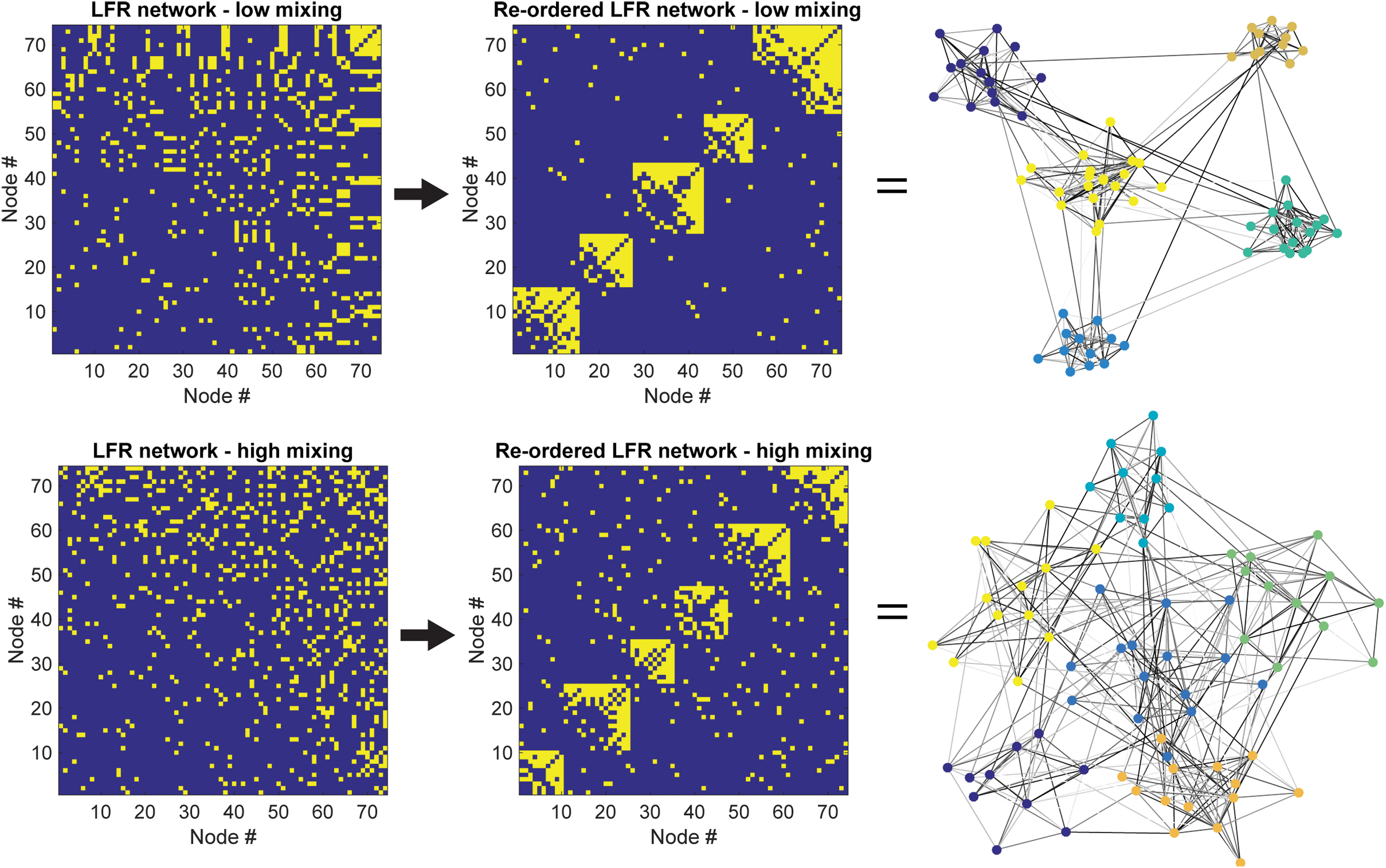
LFR benchmark networks used to compare methods to identify modules in incomplete brain networks. Example LFR benchmark networks with distinct (top row) and nondistinct (bottom row) modules are sorted after community detection to reveal modular structure. LFR, Lancichinetti–Fortunato–Radicchi. Color images are available online.

Each of four methods performs well with Louvain clustering up to substantial percentages of missing connections

When the Louvain method was used to identify modules, all four ways of accounting for missing values perform well at a range of mixing factors (indicating distinctness of modules) and proportions of missing values, for both binary and weighted networks (Fig. 2). As expected, performance of all methods is high at low mixing factors and low proportions of missing values and comparatively low at high mixing factors and high proportions of missing values. This pattern of results is similar for each of the four approaches.

FIG. 2.

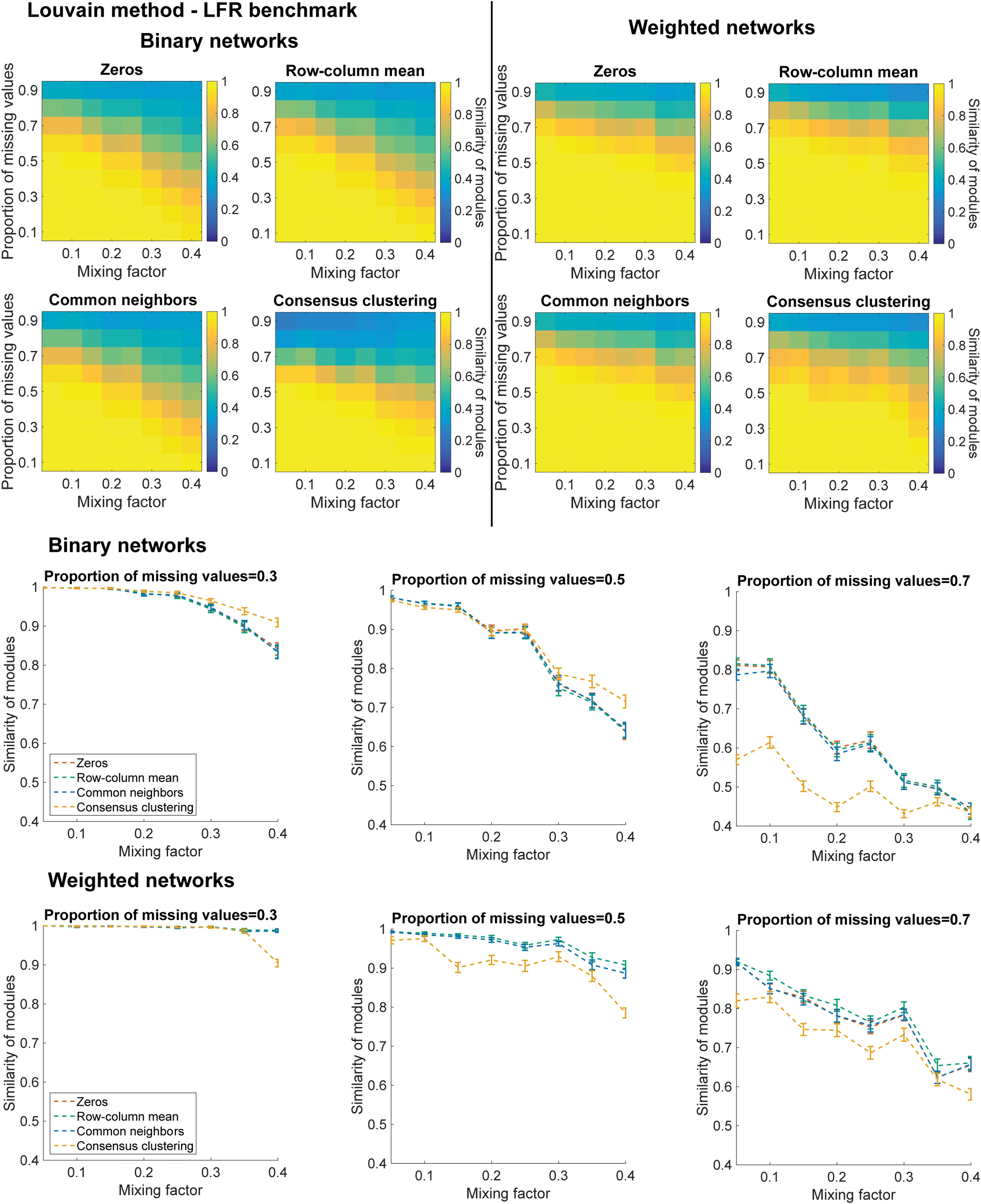
Each of four methods performs well when used with Louvain clustering up to substantial percentages of missing connections. For both binary and weighted networks, each of the four methods (zeros, row-column mean, common neighbors, and consensus clustering) performs effectively up to 50% missing connections (mean partition similarity ∼0.8 and more), for range of mixing factors studied. At higher percentages of missing connections, the “zeros,” “row-column mean,” and “common neighbors” approaches perform better than “consensus clustering,” for both binary and weighted networks. Line plots in bottom half of figure show mean and confidence intervals (±2 standard errors of mean) of similarity between identified and “ground truth” modules. Although lower bound of the line plots has been set to 0.4, note that the lower bound for the “similarity of modules” metric used is 0. Color images are available online.

Across the different methods, the “ground truth” modules are identified accurately (mean partition similarity ∼0.8 and more) when up to 50% of connections were missing, across the range of mixing factors studied. Since the weights of the weighted networks contain information aiding the identification of modules, their mean partition similarities are marginally higher than those of corresponding binary networks (Fig. 2).

As expected, the mean partition similarities are closely linked to the accuracy with which the correct number of modules was returned by the Louvain algorithm (Supplementary Fig. S1). At higher percentages of missing connections, the “zeros,” “row-column mean,” and “common neighbors” approaches perform better than “consensus clustering,” for both binary and weighted networks (Fig. 2).

The “consensus clustering” method had higher computation time than “zeros” and “row-column mean” methods and computation time similar to the “common neighbors” method (Supplementary Fig. S2), for both binary and weighted networks. Computation times with either of the four methods rarely exceed 3 seconds.

For the large binary and weighted networks, each of the four methods performed well at each of the mixing factors studied, at a range of percentages of missing values (Supplementary Fig. S3). This was a pattern identical to that obtained with the original 74 node networks. However, on the large networks of 10³ nodes, we found that computation times for “common neighbors” approach were much higher than those of “zeros,” “row-column mean,” and “consensus clustering” (Supplementary Fig. S3), even exceeding 600 seconds for high proportions of missing values, for weighted networks.

Computation times for “row-column mean” method also exceed those of “consensus clustering” for high proportions of missing values, for binary and weighted networks. The likely reason for dramatically higher computation times for “common neighbors” and “row-column mean” for large networks compared with smaller networks is the element-wise nature of filling missing values for these methods, whereas missing values are filled simultaneously with “zeros” and “consensus clustering.”

The “zeros,” “row-column mean,” and “common neighbors” method perform well with Infomap up to substantial percentages of missing connections

When the Infomap method was used to identify modules on both binary and weighted networks, the performance of the “zeros,” “row-column mean,” and “common neighbors” methods was similar to that when used with the Louvain algorithm (Fig. 3). Just as when used with Louvain, these methods gave accurate module identification (mean partition similarity ∼0.8 and more), when up to 50% of connections were missing, across the range of mixing factors studied. However, the “consensus clustering” method did not perform as well with the Infomap method, on either binary or weighted networks. Specifically, “consensus clustering” performs moderately up to 50% missing connections (mean partition similarity ∼0.4 and more), and performance suffers for higher percentages of missing connections.

FIG. 3.

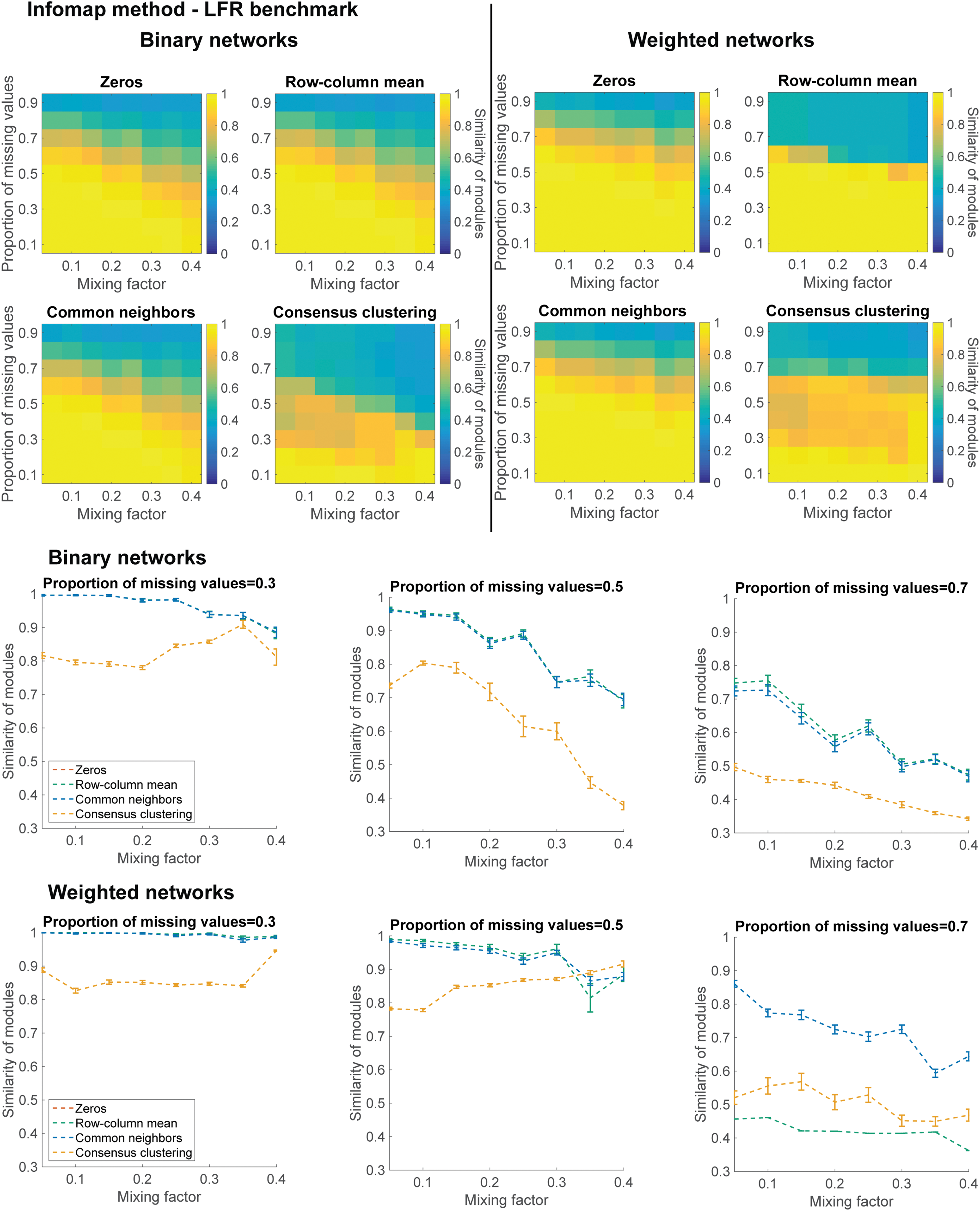
The “zeros,” “row-column mean,” and “common neighbors” methods perform well with Infomap up to substantial percentages of missing connections. For both binary and weighted networks, the “zeros,” “row-column mean,” and “common neighbors” methods perform effectively up to 50% missing connections (mean partition similarity ∼0.8 and more), for range of mixing factors studied. By contrast, “consensus clustering” performs moderately up to 50% missing connections (mean partition similarity ∼0.4 and more), and performance suffers for higher percentages of missing connections. Performance of “row-column mean” with weighted networks also suffers for high percentage of missing connections. Line plots in bottom half of figure show mean and confidence intervals (±2 standard errors of mean) of similarity between identified and “ground truth” modules. Although lower bound of the line plots has been set to 0.3, note that the lower bound for the “similarity of modules” metric used is 0. Color images are available online.

Performance of “row-column mean” with weighted networks also suffers for high percentages of missing connections. With the Infomap method also, the mean partition similarities were closely linked to the accuracy with which the correct number of modules was returned (Supplementary Fig. S1). The “consensus clustering” method also takes much longer than other approaches on these original 74 node networks (Supplementary Fig. S4). For example, “consensus clustering” takes close to 10 seconds on binary networks, whereas the next slowest method “common neighbors” takes ∼1 second.

On the large networks also, the accuracy of identifying modules with “consensus clustering” is lower than that for the other methods, for higher mixing factors and high percentages of missing connections. Just as with the 74-node networks, “row-column mean” method performs poorly for weighted networks at high percentage of missing connections (Supplementary Fig. S5). Computation times with “consensus clustering” are higher than those with the other methods, approaching 400 seconds for both binary and weighted networks. In turn, “common neighbors” method takes longer than “zeros” and “row-column mean” on binary and weighted networks. This pattern of results is identical to those observed with the smaller networks.

It should be noted, however, that the relative difference in computation times between “consensus clustering” and the next slowest method, “common neighbors” is lower for large networks than for “small networks.” For example, for small binary networks for high proportion of missing values, “consensus clustering” is ∼10 times slower than “common neighbors,” whereas for large binary networks, this factor is close to 2. The corresponding ratio comparing “consensus clustering” and “row-column mean” decreases from ∼50 for small networks to just 8 for large networks.

Before comparing the four methods on SEEG binary and weighted networks, we inspected the “percentage of stable regions” for a range of “gamma” parameter values (for Louvain) and a range of “network density” values (for Infomap). This was the percentage of regions for which modules could be identified reliably. The range of “gamma” values explored was {0.6, 0.8, 1, 1.2, and 1.4} and the range of “network density” values explored was {1%, 5%, 10%, 15%, and 20%}. The “gamma” and “network density” parameters, respectively, influence the number of modules identified with Louvain and Infomap.

We found evidence for multiscale modular organization, since statistically significant percentages of stable regions were identified for a range of gamma values (for Louvain) and network density values (for Infomap), for each of the four methods (Supplementary Fig. S6). Specifically, for Louvain, all the “gamma” values explored produced statistically significant percentage of stable regions (p < 0.05) for each of the four methods for both binary and weighted networks.

For Infomap, all the “network density” values explored produced statistically significant percentage of stable regions (p < 0.05) for binary networks, and for “zeros,” “common neighbors,” and “consensus clustering” on weighted networks. For “row-column mean” on weighted networks, only network densities of 10%, 5%, and 1% produced statistically significant percentage of stable regions. Of the many valid choices for parameter values, we chose gamma = 1 (for Louvain) and network density = 10% (for Infomap).

Each of four methods performs similarly with Louvain on SEEG binary networks, whereas “consensus clustering” performs best on SEEG weighted networks

We identified modules on SEEG networks, and also visualized the modules on inflated brain representations (Fig. 4). For SEEG binary networks, percentages of regions for which modules can be reliably identified are similar for each of the methods, that is, 48.3% (zeros), 47.3% (row-column mean), 49% (common neighbors), and 46.3% (consensus clustering; Fig. 5). For weighted networks, the “consensus clustering” approach (67.9%) outperforms the “zeros” (51.9%), “row-column mean,” (51.2%) and “common neighbors” methods (50.4%). Only the “consensus clustering” method identifies a module comprising regions in the frontal lobe for both binary and weighted networks, in addition to the posterior parietal, superior temporal, and sensorimotor module identified by the “zeros,” “row-column mean,” and “common neighbors” methods (Fig. 5).

FIG. 4.

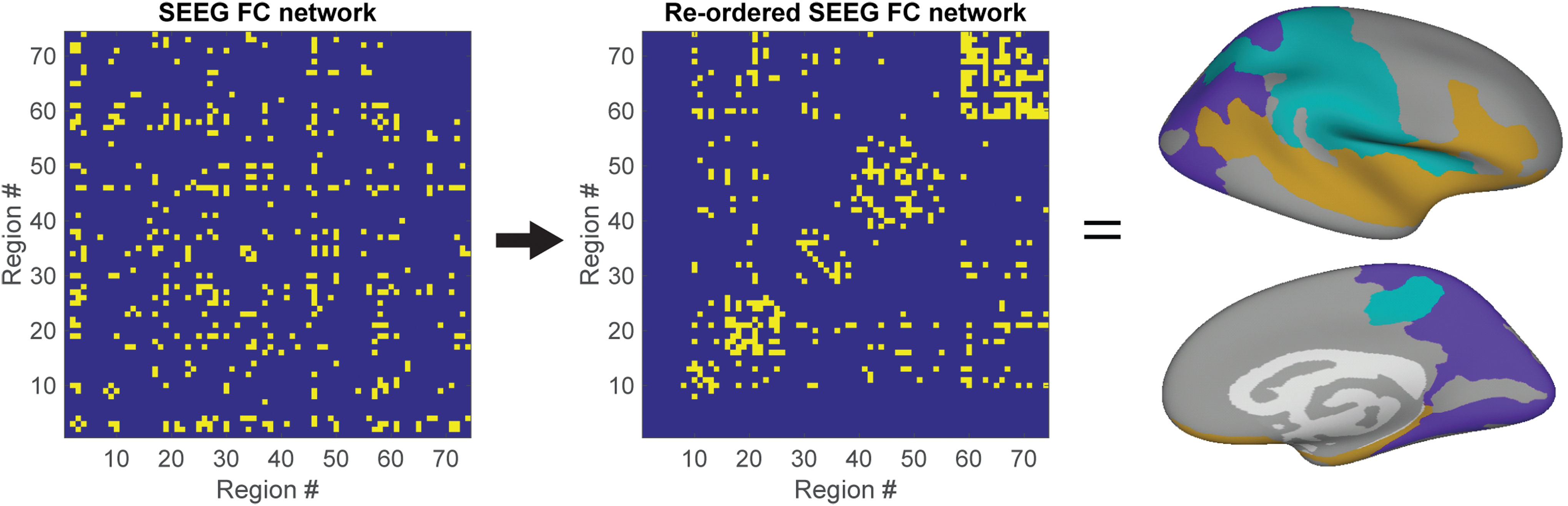
Group-level SEEG functional connectome used to compare methods to identify modules in incomplete brain networks. Group-level SEEG functional connectome derived from activity in the alpha frequency band (8–12 Hz) is sorted after community detection, and modules are visualized on inflated brain representations. FC, functional connectivity; SEEG, stereotactical electroencephalography. Color images are available online.

FIG. 5.

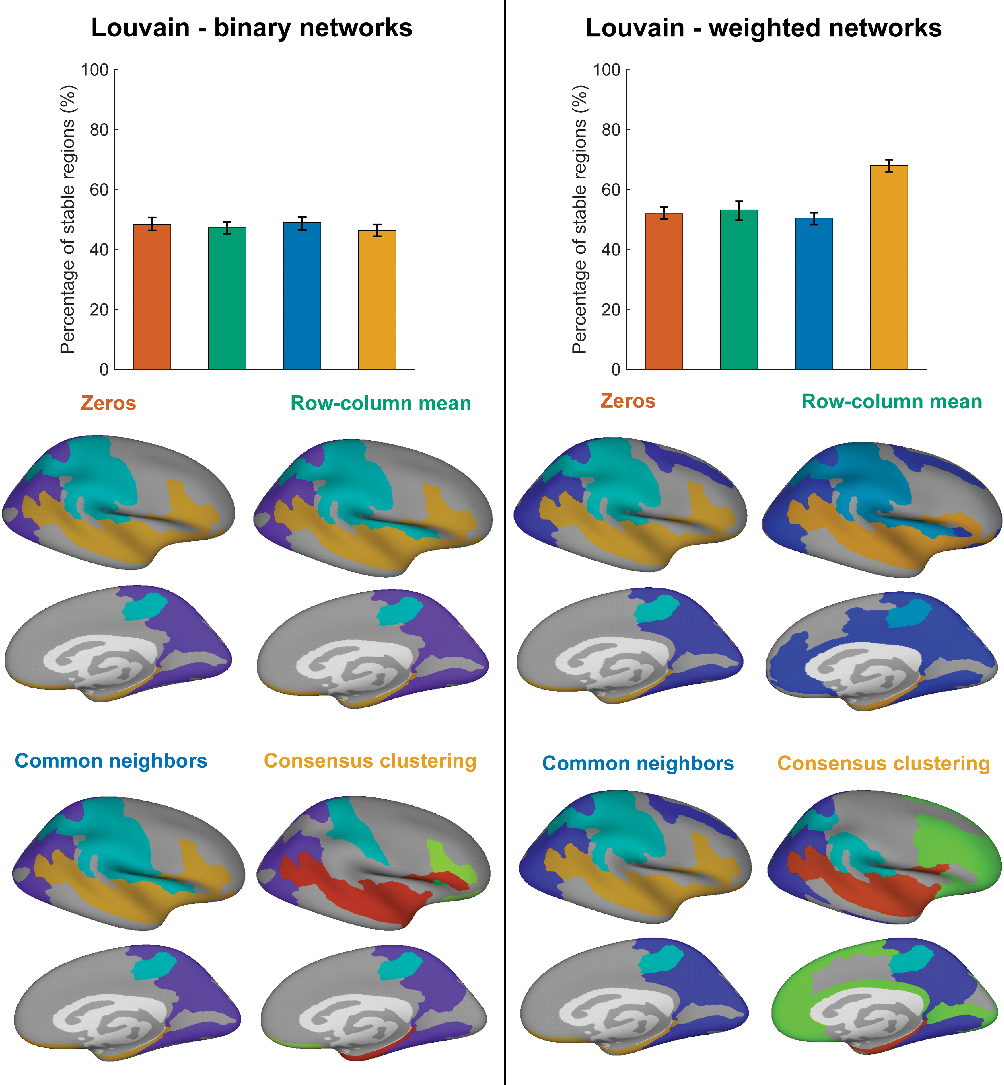
Each of four methods performs similarly with Louvain on SEEG binary networks, whereas “consensus clustering” performs best on SEEG weighted networks. Percentage of regions for which modules can be reliably identified is similar for each of four methods on SEEG binary networks, whereas this percentage is higher for “consensus clustering” than other methods for SEEG weighted networks. With the “row-column mean” method, the module assignment of no regions is reliably identified. Bar plots show mean and confidence intervals (±2 standard errors of mean) of percentage of regions for which modules can be reliably identified. Inflated brain representations show spatial layout of identified modules. Only the “consensus clustering” method identifies a module comprising regions in the frontal lobe for both binary and weighted networks, in addition to the posterior parietal, superior temporal, and sensorimotor module identified by the “zeros,” “row-column mean,” and “common neighbors” methods. Color images are available online.

Each of these modules comprises regions that are known to be functionally related, and might, respectively, reflect functional systems responsible for reasoning and planning, sensory associative processing, auditory processing, and sensorimotor processing, respectively (Gazzaniga et al., 2002; Semrud-Clikeman and Ellison, 2009). Modules comprising spatially contiguous regions have also been found in other studies of human structural (Hagmann et al., 2008) and functional brain networks (Mehrkanoon et al., 2014; Zhigalov et al., 2017), as well as structural networks in animals (Hilgetag et al., 2000; Goulas et al., 2015).

Consensus clustering can be used with Louvain to identify modules for moderate but not high percentages of missing connections

With the consensus clustering approach, modules can be identified reliably for a substantial number of regions for binary and weighted networks, when up to 30% of connections are missing (Fig. 6). This holds both when connections are deleted at random from the original SEEG connectome, or in ascending order of number of samples used to estimate the strength of functional connections, that is, connections for which lower number of samples was used for estimation were deleted first.

FIG. 6.

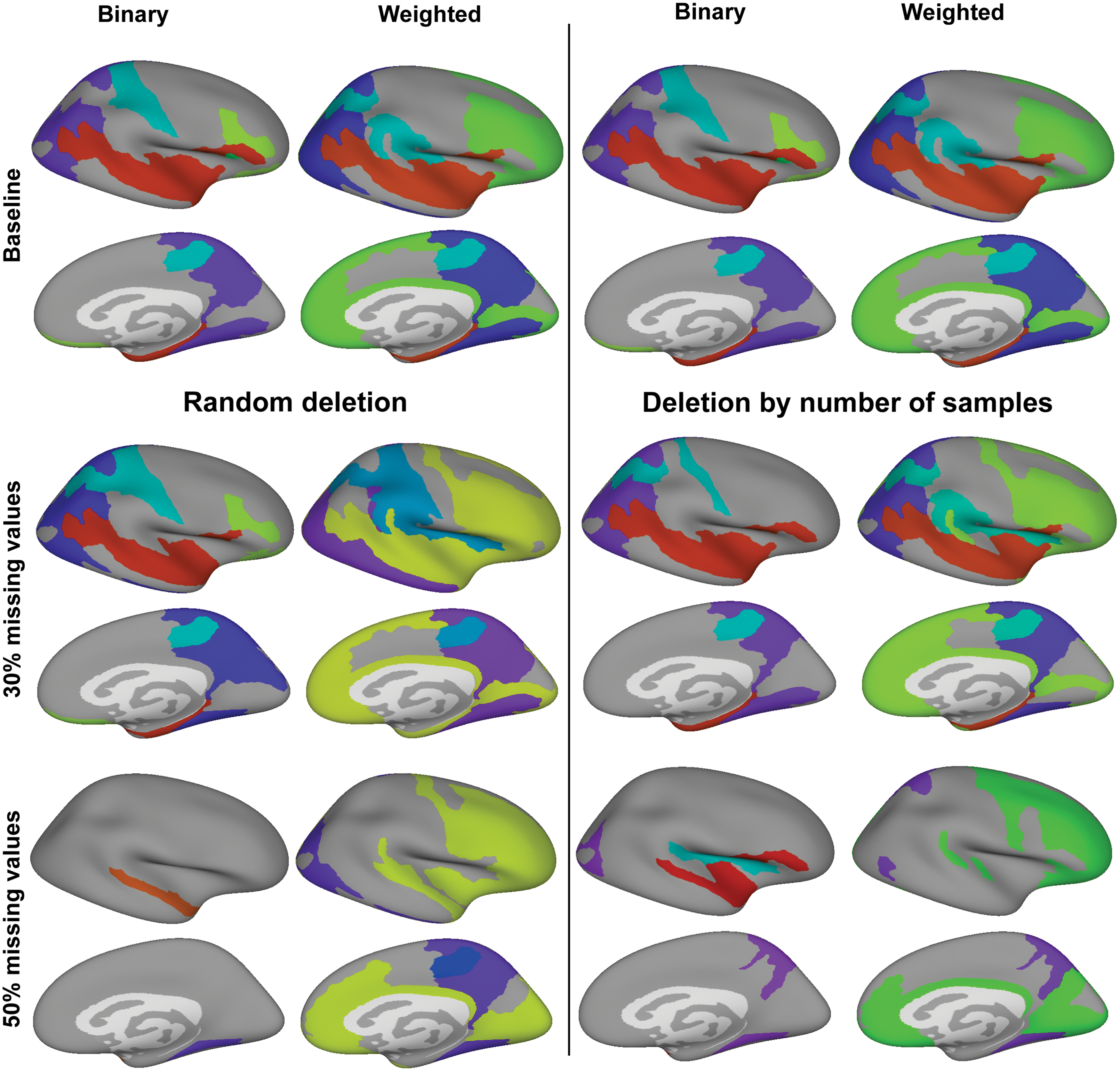
Consensus clustering can be used with Louvain to identify modules for moderate but not high percentages of missing connections. Modules can be identified reliably for a substantial number of regions for binary and weighted networks, when up to 30% of connections are missing, with the “consensus clustering” approach. This holds both when connections are deleted at random from the original SEEG connectome with 20% missing connections, or in ascending order of number of samples used to estimate the strength of functional connections. When 50% of connections are missing, modules can be identified reliably for only a few regions, especially for binary networks. This holds for both random and selective deletion of connections. Color images are available online.

When 50% of connections are missing, modules can be identified reliably for only a few regions, although a higher number for weighted than for binary networks. This holds for both random and selective deletion of connections, although regions in the frontal and superior temporal regions become merged into a single module for random deletion but not for selective deletion.

“Zeros” and “common neighbors” methods perform best with Infomap across SEEG binary and weighted networks

When used with Infomap, highest percentages of regions whose modules can be reliably identified occur for “zeros” and “common neighbors,” for both binary (49% and 48.5%, respectively) and weighted networks (52.6% and 53%, respectively; Fig. 7). For both binary (34.5%) and weighted networks (35.9%), “consensus clustering” performs less well than “zeros” and “common neighbors,” whereas “row-column mean” performs similarly to these two methods for binary networks (47.9%), but not as well for weighted networks (53%).

FIG. 7.

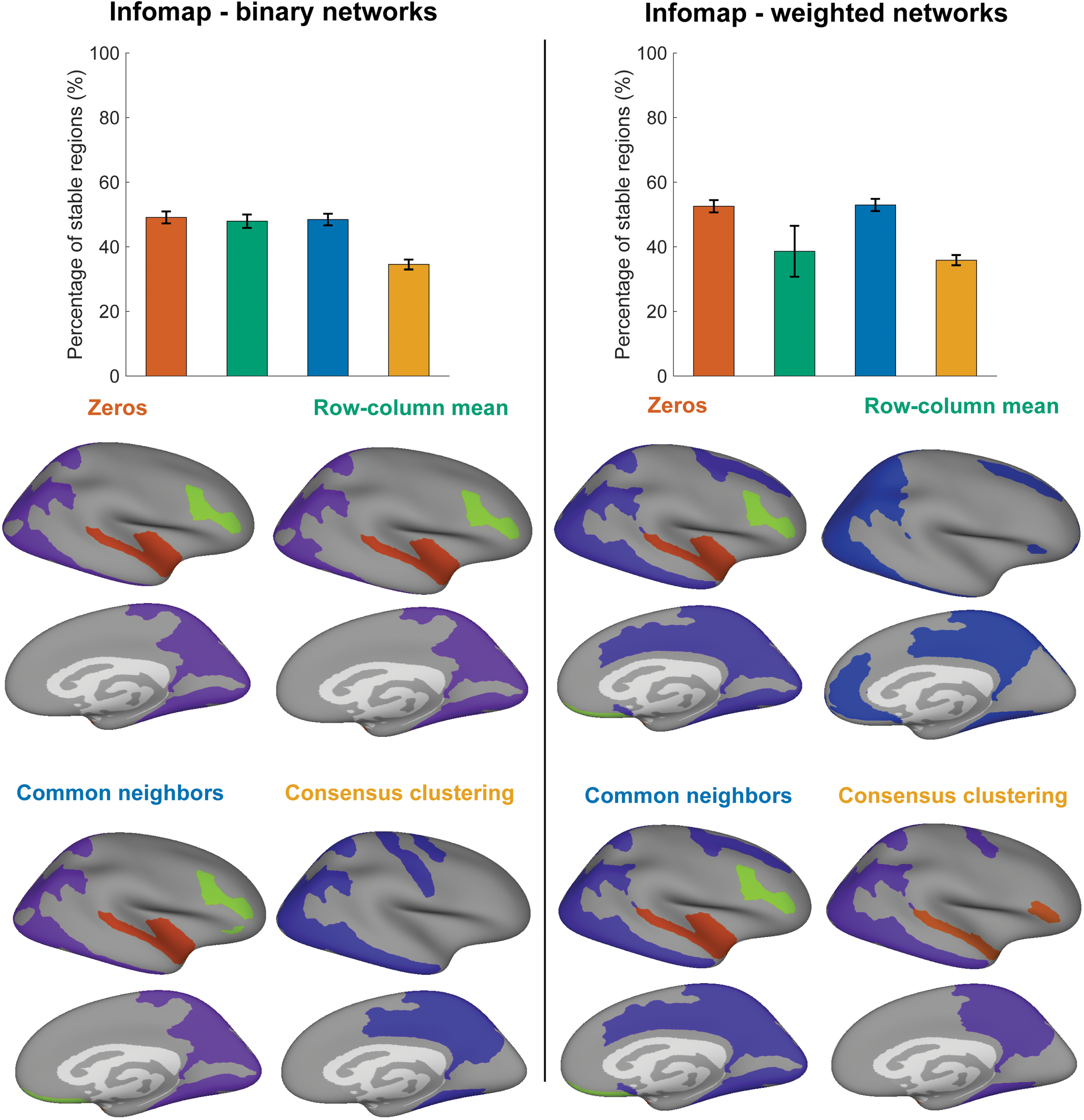
“Zeros” and “common neighbors” methods perform best with Infomap across SEEG binary and weighted networks. Percentage of regions for which modules can be reliably identified is highest for “zeros” and “common neighbors” methods across binary and weighted networks. “Consensus clustering” performs less well than “zeros” and “common neighbors” for both binary and weighted networks, whereas “row-column mean” performs as well as these two methods for binary networks, but worse for “weighted networks.” Bar plots show mean and confidence intervals (±2 standard errors of mean) of percentage of regions for which modules can be reliably identified. Inflated brain representations show spatial layout of identified modules. Both the “zeros” and “common neighbors” methods identify modules comprising mainly frontal, superior temporal, and posterior parietal regions, respectively, across binary and weighted networks, whereas the other methods identify only a subset of these modules. Color images are available online.

These results follow the same pattern as the simulations with Infomap. Both “zeros” and “common neighbors” methods identify modules comprising mainly frontal, superior temporal, and posterior parietal regions across binary and weighted networks, whereas the other methods identify only a subset of these modules.

“Zeros” method can be used with Infomap to identify modules for moderate but not high percentages of missing connections

With the zeros method, modules can be identified reliably for a number of regions for binary and weighted networks when up to 30% of connections are missing, for both binary and weighted networks (Fig. 8). This holds both when connections are deleted at random from the original SEEG connectome, or in ascending order of number of samples used to estimate the strength of functional connections. Conversely, when 50% of connections are missing, modules can be identified reliably for only a few regions, for both binary and weighted networks.

FIG. 8.

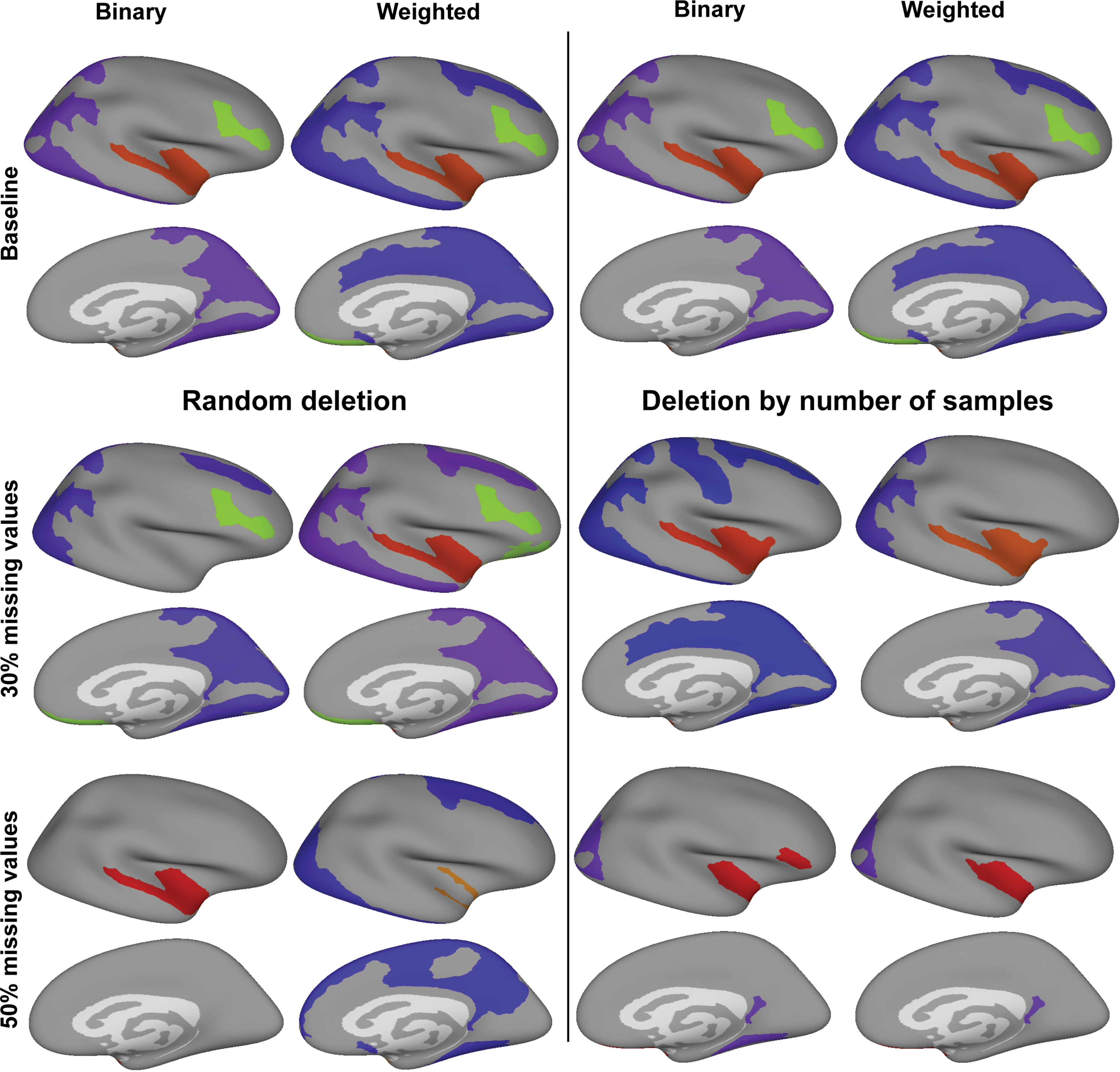
“Zeros” method can be used with Infomap to identify modules for moderate but not high percentages of missing connections. Modules can be identified reliably for a number of regions for binary and weighted networks, when up to 30% of connections are missing, with the “zeros” method. This holds when connections are deleted at random from the original SEEG connectome with 20% missing connections, or in ascending order of number of samples used to estimate the strength of functional connections. When 50% of connections are missing, modules can be identified reliably for only a few regions, for both binary and weighted networks. This holds for both random and selective deletion of connections. Color images are available online.

Discussion

Network modules reflect the functional organization of brain networks and community detection algorithms from graph theory are used to identify modules. However, interregional human brain connectomes usually contain noisy connections due to signal or source mixing or missing connections due to sparse spatial coverage, which may confound the identification of modules. In this study, we compared four methods of accounting for missing connections on binary and weighted versions of simulated and empirical networks, using both Louvain and Infomap community detection algorithms.

We find using simulated networks that when used with Louvain community detection methods, each of the four approaches can effectively identify modules even when the network has up to 50% missing connections. Similar performance is obtained when using Infomap with all methods except for “consensus clustering.” When applying the four approaches to incomplete empirical SEEG networks, we find that the “consensus clustering” approach outperforms other approaches when used with Louvain on weighted networks, whereas the “zeros” or “common neighbors” methods perform well when used with Infomap.

Suggestions for use

Based on our results, we can make some suggestions for which method to use, to account for missing values in different situations. When using Louvain to identify modules on weighted brain networks, the “consensus clustering” approach should be used, particularly due to its effective performance on SEEG weighted networks as well as reasonable computation times on both small and large simulated networks. Although performance of “consensus clustering” dips at high percentage of missing connections on simulated weighted networks, such a situation occurs rarely in analyzing brain networks. For example, the interregional functional networks from a previous study had only 4.1% connections considered to be noisy (Power et al., 2011). When Louvain is used on binary brain networks, each of the methods to account for missing connections yields similar results.

When Infomap is used, both simulations and investigations on SEEG networks suggest using “zeros” or “common neighbors” for both binary and weighted networks. However, the “zeros” method might be preferred to “common neighbors” on large networks due to the high computation times observed with “common neighbors” on such networks.

Novel aspects

This study is the first comparison of methods to account for missing connections, when identifying modules in noisy or incomplete brain networks. Although other studies have investigated the performance of different link prediction methods to identify modules in incomplete networks (Yan and Gregory, 2012), this study also assessed the performance of four approaches on empirical brain networks and explored the effect on the modular structure of both random and structured deletion of links. Furthermore, this is the first time to our knowledge that ways of accounting for missing connections on weighted networks have been studied, rather than only binary networks. A further novel aspect is that this is the first time “consensus clustering” has been adapted for use in identifying modules in incomplete brain networks.

Agreement between results on simulated and empirical networks

Results of comparing the four approaches between simulated and empirical networks are in agreement, except that “consensus clustering” works as well as other approaches for simulated weighted networks with Louvain, but better than other approaches on empirical SEEG weighted networks. Although the reason for this discrepancy is unclear, it might have to do with differences in topological properties of the simulated and empirical networks. The LFR benchmark networks mimic some common topological properties of real-world networks including brain networks, for example, power law degree distribution. However, they do not possess topological features that are specific to brain networks, which are influenced by spatial constraints and a tendency for regions having similar local neighborhoods to be connected to each other (Betzel et al., 2016).

Caveats and future work

Our conclusions on identification of modules with the four methods are based on investigations with simulated and empirical networks of 74 nodes, which correspond to one hemisphere of the Destrieux atlas. How do these results generalize to larger networks? We have demonstrated that the same pattern of results holds for networks of 10³ nodes. Furthermore, previous studies have shown that Louvain and Infomap give similar performance on networks with 5 × 10⁴ nodes and 10⁵ nodes as they do for smaller networks (Lancichinetti and Fortunato, 2009b).

Both the Louvain and Infomap algorithms are recommended for use on large networks (Yang et al., 2016), and their ability to correctly identify communities has been demonstrated to be similar across a wide range of network sizes, including large networks with 2 × 10⁴ nodes (Yang et al., 2016). Since our results are based on identifying communities with either Louvain or Infomap after generating complete networks with either of the four methods, we expect the conclusions from our study to also hold for very large networks, for example, voxel-wise fMRI networks of 10⁶ nodes.

Our conclusions on computation times with the four methods are also based on investigations with simulated and empirical networks of 74 nodes. How do these results generalize to large networks? The differences in computation times of the four methods arise from differences in the time taken to generate the complete matrix, for use by either Louvain or Infomap to identify modules. Hence, the “zeros” method is quickest because all missing values can be filled simultaneously. Missing values for “row-column mean” and “common neighbors” are replaced element wise, which accounts for high computation times with these methods on large networks. “Consensus clustering” generates the complete matrix by performing multiple identifications of community structure with either Louvain or Infomap and hence, this method also has high computation times.

Previous work (Yang et al., 2016) has shown that computation times for identifying modules with Louvain increase only slowly with network size, whereas computation times with Infomap increase rapidly with network size. The low increase of computation time with network size for Louvain explains our results, specifically why “consensus clustering” with Louvain is relatively fast for large networks of 10³ nodes, compared with computations times for “common neighbors” and “row-column mean,” whose element-wise computations make them slow. Owing to this low rate of increase in computation times of Louvain with increasing network size, we expect that “common neighbors” and “row-column mean” will take much longer than “consensus clustering” on very large networks of 10⁶ nodes or more, for example, voxel-wise fMRI networks. The “zeros” method will remain the quickest.

For the Infomap method, the rapid increase in computation time with network size also explains our results, specifically why “consensus clustering” with Infomap is slower than “common neighbors” and “row-column mean,” even for large networks of 10³ nodes. However, the ratio between computation times for “consensus clustering” and “common neighbors” with Infomap decreases from values close to 10 for small binary networks to values close to 2 for large binary networks of 10³ nodes. This indicates that increase in computation time of “common neighbors” with network size is higher than increase in computation time of “consensus clustering” with network size. A similar trend occurs for computation times of “row-column mean” for small and large networks compared with corresponding times for “consensus clustering.”

Hence, we expect the computation times of “common neighbors” and “row-column” to exceed those of “consensus clustering” for very large networks of 10⁶ nodes or more, for example, voxel-wise fMRI networks. Here also, the computational simplicity of generating a complete matrix with the “zeros” method will make it the quickest among the four methods.

This study investigated identifying communities in binary and weighted undirected networks. Future work could extend this toward determining effective ways of accounting for missing connections, when the underlying network is directed (Lancichinetti and Fortunato, 2009a).

Conclusion

Although modules can provide insight into network organization, noisy or missing connections in brain networks hamper the identification of modules. In this article, we performed simulations on simulated and empirical networks to determine the effectiveness of different ways of accounting for noisy or missing connections when identifying modules. We find that different approaches work better in different situations, and make suggestions for use based on these observations. These findings and suggestions provide a sound basis on which future studies can identify modules in noisy or incomplete brain networks.

Footnotes

Acknowledgments

The authors thank Jonni Hirvonen for help with programming and data processing. The authors are also grateful to Dr. Francesco Cardinale and Annalisa Rubino for facilitating the recording of stereotactical electroencephalography resting-state data. The authors also appreciate the helpful review comments, which have improved the quality of the article.

Author Disclosure Statement

No competing financial interests exist.

Supplementary Material

Supplementary Figure S1

Supplementary Figure S2

Supplementary Figure S3

Supplementary Figure S4

Supplementary Figure S5

Supplementary Figure S6

References

Arnulfo

, Hirvonen

, Nobili

, Palva

. 2015a. Phase and amplitude correlations in resting-state activity in human stereotactical EEG recordings. Neuroimage, 112:114–127.

Arnulfo

, Narizzano

, Cardinale

, Fato

, Palva

. 2015b. Automatic segmentation of deep intracerebral electrodes in computed tomography scans. BMC Bioinformatics, 16:99.

Airoldi

, Blei

, Fienberg

, Xing

. 2008. Mixed-membership stochastic blockmodels. J Mach Learn Res, 9:1981–2014.

Beckmann

, DeLuca

, Devlin

, Smith

. 2005. Investigations into resting-state connectivity using independent component analysis. Philos Trans R Soc Lond B Bio Sci, 360:1001–1013.

Betzel

, Avena-Koenigsberger

, Goni

, He

, de Reus

, Griffa

, et al. 2016. Generative models of the human connectome. Neuroimage, 124:1054–1064.

Blondel

, Guillaume

J-L

, Lambiotte

, Lefebvre

. 2008. Fast unfolding of communities in large networks. J Stat Mech P10008:arXiv:0803.0476.

Bota

, Sporns

, Swanson

. 2015. Architecture of the cerebral cortical association connectome underlying cognition. Proc Natl Acad Sci USA, 112:E2093–E2101.

Buckner

, Vincent

. 2007. Unrest at rest: default activity and spontaneous network correlations. Neuroimage, 37:1091–1096.

Bullmore

, Sporns

. 2009. Complex brain networks: graph theoretical analysis of structural and functional systems. Nat Rev Neurosci, 10:186–198.

10.

Cardinale

, Cossu

, Castana

, Casaceli

, Schiariti

, Miserocchi

, et al. 2013. Stereoelectroencephalography: surgical methodology, safety, and stereotactic application accuracy in 500 procedures. Neurosurgery, 72:353–366.

11.

Catani

, de Schotten

. 2012. Atlas of human brain connections. J Psychiatry, 55:545–546.

12.

Chavez

, Valencia

, Navarro

, Latora

, Martinerie

. 2010. Functional modularity of background activities in normal and epileptic brain networks. Phys Rev Lett, 104:118791.

13.

Clauset

, Moore

, Newman

. 2008. Hierarchical structure and prediction of missing links in networks. Nature, 453:98–101.

14.

Damoiseaux

, Rombouts

, Barkhof

, Scheltens

, Stam

, Smith

, Beckmann

. 2006. Consistent resting-state networks across healthy subjects. Proc Natl Acad Sci USA, 103:13848–13853.

15.

de Haan

, Pijnenburg

YAL

. Strijers

RLM

, van der Made

, van der Flier

, Scheltens

, Stam

CJ.

2009. Functional neural network analysis in frontotemporal dementia and Alzheimer's disease using EEG and graph theory. BMC Neurosci, 10:101.

16.

Dell'Acqua

, Rizzo

, Scifo

, Clarke

, Scotti

, Fazio

. 2007. A model-based deconvolution approach to solve fiber crossing in diffusion weighted MR imaging. IEEE Trans Biomed Eng, 54:462–472.

17.

Destrieux

, Fischl

, Dale

, Halgren

. 2010. Automatic parcellation of human cortical gyri and sulci using standard anatomical nomenclature. Neuroimage, 53:1–15.

18.

Dorelan

, Batagelj

, Ferligoj

. 2005. Generalized Blockmodeling. Cambridge, UK: Cambridge University Press.

19.

Gazzaniga

, Ivry

, Mangun

. 2002. Cognitive Neuroscience: The Biology of the Mind, 2nd ed. New York: Norton WW.

20.

Goldberg

, Roth

. 2003. Assessing experimentally derived interactions in a small world. Proc Natl Acad Sci USA, 100:4372–4376.

21.

Goulas

, Schaefer

, Margulies

. 2015. The strength of weak connections in the macaque cortico-cortical network. Brain Struct Funct, 220:2939–2951.

22.

Hagmann

, Cammoun

, Gigander

, Meuli

, Honey

, Wedeen

, Sporns

. 2008. Mapping the structural core of human cerebral cortex. PLoS Biol, 6:e159.

23.

Harriger

, van den Heuvel

, Sporns

. 2012. Rich club organisation of macaque cerebral cortex and its role in network communication. PLoS One, 7:e46497.

24.

Hilgetag

, Burns

, O'Neill

, Scannell

, Young

. 2000. Anatomical connectivity defines the organization of clusters of cortical areas in the macaque and the cat. Philos Trans R Soc Lond B Biol Sci, 355:91–110.

25.

Hillebrand

, Barnes

, Bosboom

, Berendse

, Stam

. 2012. Frequency-dependent functional connectivity within resting-state networks: an atlas-based MEG beamformer solution. Neuroimage, 59:3909–3921.

26.

Jaccard

1912. The distribution of flora in the alpine zone. New Phytologist, 11:37–50.

27.

Jeh

, Widom

. 2002. SimRank: a measure of structural-context similarity. In Proceedings of the ACM SIGDD International Conference on Knowledge Discovery and Data Mining, ACM Press, New York, pp. 271–279.

28.

Lachaux

, Rodriguez

, Martineria

, Varela

. 1999. Measuring phase synchrony in brain signals. Hum Brain Mapp, 8:194–208.

29.

Lancichinetti

, Fortunato

. 2009a. Benchmarks for testing community detection algorithms on directed and weighted graphs with overlapping communities. Phys Rev E, 80:016118.

30.

Lancichinetti

, Fortunato

. 2009b. Community detection algorithms: a comparative analysis. Phys Rev E, 80:056117.

31.

Lancichinetti

, Fortunato

. 2012. Consensus clustering in complex networks. Sci Rep, 2:336.

32.

Lancichinetti

, Fortunato

, Radicchi

. 2008. Benchmark graphs for testing community detection algorithms. Phys Rev E, 78:046110.

33.

Lü

, Jin

, Zhou

. 2009. Similarity index based on local paths for link prediction of complex networks. Phys Rev E, 80:046122.

34.

Lü

, Zhou

. 2011. Link prediction in complex networks: a survey. Physica A, 390:1150–1170.

35.

Mehrkanoon

, Breakspear

, Boonstra

. 2014. Low-dimensional dynamics of resting-state cortical activity. Brain Topogr, 27:338–352.

36.

Meunier

, Lambiotte

, Fornito

, Ersche

, Bullmore

. 2009. Hierarchical modularity in human brain functional networks. Front Neuroinform, 3:37.

37.

Nicolini

, Bifone

. 2016. Modular structure of brain functional networks: breaking the resolution limit by Surprise. Sci Rep, 6:19250.

38.

Nicolini

, Bordier

, Bifone

. 2017. Community detection in weighted brain connectivity networks beyond the resolution limit. Neuroimage, 146:28–39.

39.

Palva

, Wang

, Palva

, Zhigalov

, Monto

, Brookes

, et al. 2018. Ghost interactions in MEG/EEG source space: a note of caution on inter-areal coupling measures. Neuroimage, 173:632–643.

40.

Palva

, Palva

. 2012. Discovering oscillatory interaction networks with M/EEG: challenges and breakthroughs. Trends Cogn Sci, 16:219–230.

41.

Power

, Cohen

, Nelson

, Wig

, Barnes

, Church

, et al. 2011. Functional network organisation of the human brain. Neuron, 72:665–678.

42.

Rosvall

, Bergstrom

. 2008. Maps of random walks on complex networks reveal community structure. Proc Natl Acad Sci USA, 105:1118–1123.

43.

Rubinov

, Sporns

. 2010. Complex networks measures of brain connectivity: uses and interpretations. Neuroimage, 52:1059–1069.

44.

Salvador

, Suckling

, Coleman

, Pickard

, Menon

, Bullmore

. 2005. Neurophysiological architecture of functional magnetic resonance images of human brain. Cereb Cortex, 15:1332–1342.

45.

Schmahmann

, Pandya

. 2006. Fiber Pathways of the Brain. Oxford: Oxford University Press.

46.

Semrud-Clikeman

, Teeter Ellison

. 2009. Functional neuroanatomy. In: Child Neuropsychology: Assessments and Interventions for Neurodevelopmental Disorders. New York: Springer Science & Business Media, pp. 25–46.

47.

Sporns

, Betzel

. 2016. Modular brain networks. Annu Rev Psychol, 67:613–640.

48.

Stam

, de Haan

, Daffertschofer

ABFJ

, Jones

, Manshanden

, van Cappellen van Walsum

A-M

, et al. 2008. Graph theoretical analysis of magnetoencephalographic functional connectivity in Alzheimer's disease. Brain, 132:213–224.

49.

Thomas

, Ye

, Irfanoglu

, Modi

, Saleem

, Leopold

, Pierpaoli

. 2014. Anatomical accuracy of brain connections derived from diffusion MRI tractography is inherently limited. Proc Natl Acad Sci USA, 111:16574–16579.

50.

van den Heuvel

, Sporns

. 2013. Network hubs in the human brain. Trends Cogn Sci, 17:683–696.

51.

Vértes

, Alexander-Bloch

, Gogtay

, Giedd

, Rapoport

, Bullmore

. 2012. Simple models of human brain functional networks. PNAS, 109:5868–5873.

52.

Wang

, Sporns

, Burkhalter

. 2012. Network analysis of corticocortical connections reveal ventral and dorsal processing streams in mouse visual cortex. J Neurosci, 32:4386–4399.

53.

Wig

GS.

2017. Segregated systems of human brain networks. Trends Cogn Sci, 21:981–996.

54.

Yan

, Gregory

. 2012. Finding missing edges in networks based on their community structure. Phys Rev E, 85:056112.

55.

Yang

, Algesheimer

, Tessone

. 2016. A comparative analysis of community detection algorithms on artificial neural networks. Sci Rep, 6:30750.

56.

, Chu

, Yu

, Tresp

, Xu

. 2006. Stochastic relational models for discriminative link prediction. In Proceedings of Neural Information Processing Systems, MIT Press, Cambridge, MA, pp. 1553.

57.

Zhang

, Benz

, Bezerianos

, Acharya

, Crone

, Maybhate

, et al. 2010. Connectivity mapping of the human ECoG during a motor task with a time-varying dynamic Bayesian network. Conf Proc IEEE Eng Med Biol Soc, 2010:130.

58.

Zhigalov

, Arnulfo

, Nobili

, Palva

. 2017. Modular co-organisation of functional connectivity and scale-free dynamics in the human brain. Netw Neurosci, 1:143–165.

Supplementary Material

Please find the following supplemental material available below.

For Open Access articles published under a Creative Commons License, all supplemental material carries the same license as the article it is associated with.

For non-Open Access articles published, all supplemental material carries a non-exclusive license, and permission requests for re-use of supplemental material or any part of supplemental material shall be sent directly to the copyright owner as specified in the copyright notice associated with the article.

0.00 MB

0.32 MB

0.33 MB

0.27 MB

0.22 MB

0.27 MB

0.43 MB