A large body of evidence relates autism with abnormal structural and functional brain connectivity. Structural covariance magnetic resonance imaging (scMRI) is a technique that maps brain regions with covarying gray matter densities across subjects. It provides a way to probe the anatomical structure underlying intrinsic connectivity networks (ICNs) through analysis of gray matter signal covariance. In this article, we apply topological data analysis in conjunction with scMRI to explore network-specific differences in the gray matter structure in subjects with autism versus age-, gender-, and IQ-matched controls. Specifically, we investigate topological differences in gray matter structure captured by structural correlation graphs derived from three ICNs strongly implicated in autism, namely the salience network, default mode network, and executive control network. By combining topological data analysis with statistical inference, our results provide evidence of statistically significant network-specific structural abnormalities in autism.
Introduction
Autism is a complex developmental disorder characterized by impairment in social interactions, difficulty in verbal and nonverbal communication, and repetitive behaviors. Although the exact mechanism of its development remains unclear, there is strong evidence relating autism to abnormal structural and functional connectivity between brain regions. Structural abnormalities can be identified using voxel-based morphometry by comparing gray matter and white matter volumes or densities, as well as using cortical thickness and their respective growth trajectories (Schumann et al., 2010; Zielinski et al., 2014) across diagnostic groups. Although the gross brain differences have been well-documented (Courchesne et al., 2007), investigations into specific regional abnormalities in brain structure have reported divergent results (Stigler et al., 2011).
These inconsistent findings, however, may reflect discrete abnormalities in any given brain network. Research has revealed a finite set of canonical, domain-specific resting-state or intrinsic connectivity networks (ICNs) that organize brain function (Fox et al., 2005). Many of the regions with reported abnormalities in autism lie within these ICNs. Network-specific differences could account for seemingly contradictory findings from previous studies.
Structural covariance magnetic resonance imaging (scMRI) maps regions of gray matter that have a statistically significant correlation with a specific seed region of interest (ROI) across subjects. This suggests shared developmental or genetic influences between the gray matter region and the seed ROI (Zielinski et al., 2010). Seeley and colleagues (2009) have used scMRI to demonstrate that specific adult dementias affect distinct ICNs and the corresponding gray matter regions. Using a similar technique, Zielinski and colleagues (2012) have shown that there are network-specific structural differences between autism and control groups, which are consistent with clinical aspects of the disease, and that reported functional abnormalities in autism have a structural bias. Several recent studies have applied the scMRI technique to find evidence of network-specific structural abnormalities in other diseases such as Alzheimer's (Montembeault et al., 2016) and Huntington's (Minkova et al., 2016) diseases.
However, scMRI can only reveal shared influences between gray matter voxels and a specific seed ROI. Alternatively, we can model correlations across subjects, between all possible pairs of gray matter regions, as a network. Such a network represents structural relationships between regions, which are not captured by conventional scMRI. Comparing these networks across diagnostic groups may provide information that is not given by direct comparisons anchored by network seeds.
Network comparison is not an easy problem, especially when the networks are weighted. Several graph-theoretic measures have been proposed previously to compare networks (Bullmore and Sporns, 2009). However, a major drawback of these measures is their reliance on a fixed topology. That is, these measures are typically based on a binary graph obtained by thresholding the connectivity matrix. The choice of threshold is crucial in such analyses. Different heuristics have been suggested to determine the threshold depending on which properties of the network are of interest. However, it is often not possible to determine a unique optimal threshold.
In this article, we apply topological data analysis to graphs derived from three ICNs strongly implicated in autism: the default mode network (DMN), salience network (SN), and executive control network (ECN); these graphs are referred to as structural correlation graphs (SCGs). Our method is based on a core technique from topological data analysis known as persistent homology (Edelsbrunner et al., 2002) and follows closely the work of Lee and colleagues (2012). We compare topological invariants of two graphs across all thresholds (obtained via persistent homology) to make statistical inference. By combining topological data analysis with statistical inference, our results provide evidence of statistically significant structural abnormalities underlying ICNs in autism. Our results are consistent with the observations of Zielinski and colleagues (2012) and may offer new insights toward interpreting fine-scale, network-specific structural differences.
Materials and Methods
Structural correlation graphs
We first use scMRI to identify a set of brain regions underlying a specific ICN, according to methods published previously (Zielinski et al., 2010). This is done by first determining a seed ROI known to anchor a specific ICN and then implementing a generalized linear model to identify regions that have covarying gray matter densities with that seed ROI, across subjects. Specifically, for a given seed ROI, separate condition group-by-covariate analysis is performed for each voxel. The mean seed gray matter density is the covariate of interest, and disease status is the grouping variable. Total brain volume and age are included as covariates of no interest. This design enables us to determine the whole-brain patterns of seed-based structural covariance in each group. To identify regions with significant gray matter density covariance with the seed ROI across subjects in a diagnostic group, one-sample t-tests with family-wise error correction are performed.
The regions are identified based on their structural relationship with a specific seed ROI. We model the structural relationships between all pairs of regions as a graph. Correlations between gray matter densities across subjects, for all pairs of regions, are modeled as a weighted undirected graph \documentclass{aastex}\usepackage{amsbsy}\usepackage{amsfonts}\usepackage{amssymb}\usepackage{bm}\usepackage{mathrsfs}\usepackage{pifont}\usepackage{stmaryrd}\usepackage{textcomp}\usepackage{portland, xspace}\usepackage{amsmath, amsxtra}\usepackage{upgreek}\pagestyle{empty}\DeclareMathSizes{10}{9}{7}{6}\begin{document}$$G \left( {V , E , W} \right)$$ \end{document}. The vertices of the graph represent gray matter regions, and edge weights are given by magnitudes of pairwise correlations.
These derived patterns of distributed structural coherence are referred to as the SCG. We compare SCGs derived from three ICNs strongly implicated in autism, the SN, ECN, and DMN. In the context of this article, for simplicity (unless otherwise specified), we describe these SCGs by the name of their corresponding ICN, namely SN-SCG, ECN-SCG, and DMN-SCG.
Graph filtration
We extract topological features at multiple scales from an SCG G by constructing a nested sequence of graphs from G, referred to as graph filtration.
Let \documentclass{aastex}\usepackage{amsbsy}\usepackage{amsfonts}\usepackage{amssymb}\usepackage{bm}\usepackage{mathrsfs}\usepackage{pifont}\usepackage{stmaryrd}\usepackage{textcomp}\usepackage{portland, xspace}\usepackage{amsmath, amsxtra}\usepackage{upgreek}\pagestyle{empty}\DeclareMathSizes{10}{9}{7}{6}\begin{document}$$V = \left\{ {{v_i}:i = 1 , 2 , \ldots , n} \right\} $$ \end{document} be the vertex set with n vertices. Let E denote the edge set and W denote the set of edge weights. The edge between vertices \documentclass{aastex}\usepackage{amsbsy}\usepackage{amsfonts}\usepackage{amssymb}\usepackage{bm}\usepackage{mathrsfs}\usepackage{pifont}\usepackage{stmaryrd}\usepackage{textcomp}\usepackage{portland, xspace}\usepackage{amsmath, amsxtra}\usepackage{upgreek}\pagestyle{empty}\DeclareMathSizes{10}{9}{7}{6}\begin{document}$${v_i} , \;{v_j}$$ \end{document} is denoted by \documentclass{aastex}\usepackage{amsbsy}\usepackage{amsfonts}\usepackage{amssymb}\usepackage{bm}\usepackage{mathrsfs}\usepackage{pifont}\usepackage{stmaryrd}\usepackage{textcomp}\usepackage{portland, xspace}\usepackage{amsmath, amsxtra}\usepackage{upgreek}\pagestyle{empty}\DeclareMathSizes{10}{9}{7}{6}\begin{document}$${e_{ij}}$$ \end{document} and its weight is denoted by \documentclass{aastex}\usepackage{amsbsy}\usepackage{amsfonts}\usepackage{amssymb}\usepackage{bm}\usepackage{mathrsfs}\usepackage{pifont}\usepackage{stmaryrd}\usepackage{textcomp}\usepackage{portland, xspace}\usepackage{amsmath, amsxtra}\usepackage{upgreek}\pagestyle{empty}\DeclareMathSizes{10}{9}{7}{6}\begin{document}$${w_{ij}}$$ \end{document}. \documentclass{aastex}\usepackage{amsbsy}\usepackage{amsfonts}\usepackage{amssymb}\usepackage{bm}\usepackage{mathrsfs}\usepackage{pifont}\usepackage{stmaryrd}\usepackage{textcomp}\usepackage{portland, xspace}\usepackage{amsmath, amsxtra}\usepackage{upgreek}\pagestyle{empty}\DeclareMathSizes{10}{9}{7}{6}\begin{document}$$\left\vert E \right\vert$$ \end{document} denotes the number of edges.
For a given threshold \documentclass{aastex}\usepackage{amsbsy}\usepackage{amsfonts}\usepackage{amssymb}\usepackage{bm}\usepackage{mathrsfs}\usepackage{pifont}\usepackage{stmaryrd}\usepackage{textcomp}\usepackage{portland, xspace}\usepackage{amsmath, amsxtra}\usepackage{upgreek}\pagestyle{empty}\DeclareMathSizes{10}{9}{7}{6}\begin{document}$$\lambda$$ \end{document}, we obtain a binary graph \documentclass{aastex}\usepackage{amsbsy}\usepackage{amsfonts}\usepackage{amssymb}\usepackage{bm}\usepackage{mathrsfs}\usepackage{pifont}\usepackage{stmaryrd}\usepackage{textcomp}\usepackage{portland, xspace}\usepackage{amsmath, amsxtra}\usepackage{upgreek}\pagestyle{empty}\DeclareMathSizes{10}{9}{7}{6}\begin{document}$${G_ \lambda }$$ \end{document} by removing edges with weight \documentclass{aastex}\usepackage{amsbsy}\usepackage{amsfonts}\usepackage{amssymb}\usepackage{bm}\usepackage{mathrsfs}\usepackage{pifont}\usepackage{stmaryrd}\usepackage{textcomp}\usepackage{portland, xspace}\usepackage{amsmath, amsxtra}\usepackage{upgreek}\pagestyle{empty}\DeclareMathSizes{10}{9}{7}{6}\begin{document}$${w_{ij}} \le \lambda$$ \end{document}. The adjacency matrix \documentclass{aastex}\usepackage{amsbsy}\usepackage{amsfonts}\usepackage{amssymb}\usepackage{bm}\usepackage{mathrsfs}\usepackage{pifont}\usepackage{stmaryrd}\usepackage{textcomp}\usepackage{portland, xspace}\usepackage{amsmath, amsxtra}\usepackage{upgreek}\pagestyle{empty}\DeclareMathSizes{10}{9}{7}{6}\begin{document}$${A_ \lambda } = \left( {{a_{ij}} \left( \lambda \right) } \right)$$ \end{document} is given as follows:\documentclass{aastex}\usepackage{amsbsy}\usepackage{amsfonts}\usepackage{amssymb}\usepackage{bm}\usepackage{mathrsfs}\usepackage{pifont}\usepackage{stmaryrd}\usepackage{textcomp}\usepackage{portland, xspace}\usepackage{amsmath, amsxtra}\usepackage{upgreek}\pagestyle{empty}\DeclareMathSizes{10}{9}{7}{6}\begin{document} \begin{align*}{a_{ij}} \left( \lambda \right) \; = \; \left\{ { \begin{matrix} {1 \; \; \;if \; \; \;{w_{ij}} \ge \lambda } \\ { 0 \; \;Otherwise} \\ \end{matrix} } \right.. \end{align*} \end{document}
As \documentclass{aastex}\usepackage{amsbsy}\usepackage{amsfonts}\usepackage{amssymb}\usepackage{bm}\usepackage{mathrsfs}\usepackage{pifont}\usepackage{stmaryrd}\usepackage{textcomp}\usepackage{portland, xspace}\usepackage{amsmath, amsxtra}\usepackage{upgreek}\pagestyle{empty}\DeclareMathSizes{10}{9}{7}{6}\begin{document}$$\lambda$$ \end{document} increases, more and more edges are removed from the graph. We can generate a sequence of thresholds, \documentclass{aastex}\usepackage{amsbsy}\usepackage{amsfonts}\usepackage{amssymb}\usepackage{bm}\usepackage{mathrsfs}\usepackage{pifont}\usepackage{stmaryrd}\usepackage{textcomp}\usepackage{portland, xspace}\usepackage{amsmath, amsxtra}\usepackage{upgreek}\pagestyle{empty}\DeclareMathSizes{10}{9}{7}{6}\begin{document}$$0 \; = \; { \lambda _0} \le { \lambda _1} \le { \lambda _2} \le \ldots \le { \lambda _q}$$ \end{document}, where \documentclass{aastex}\usepackage{amsbsy}\usepackage{amsfonts}\usepackage{amssymb}\usepackage{bm}\usepackage{mathrsfs}\usepackage{pifont}\usepackage{stmaryrd}\usepackage{textcomp}\usepackage{portland, xspace}\usepackage{amsmath, amsxtra}\usepackage{upgreek}\pagestyle{empty}\DeclareMathSizes{10}{9}{7}{6}\begin{document}$$q \le \left\vert E \right\vert$$ \end{document}, by setting \documentclass{aastex}\usepackage{amsbsy}\usepackage{amsfonts}\usepackage{amssymb}\usepackage{bm}\usepackage{mathrsfs}\usepackage{pifont}\usepackage{stmaryrd}\usepackage{textcomp}\usepackage{portland, xspace}\usepackage{amsmath, amsxtra}\usepackage{upgreek}\pagestyle{empty}\DeclareMathSizes{10}{9}{7}{6}\begin{document}$${ \lambda _i}$$ \end{document} equal to edge weights arranged in ascending order.
Corresponding to the sequence of thresholds, we get a nested sequence of binary graphs referred to as a graph filtration G (Lee et al., 2012):\documentclass{aastex}\usepackage{amsbsy}\usepackage{amsfonts}\usepackage{amssymb}\usepackage{bm}\usepackage{mathrsfs}\usepackage{pifont}\usepackage{stmaryrd}\usepackage{textcomp}\usepackage{portland, xspace}\usepackage{amsmath, amsxtra}\usepackage{upgreek}\pagestyle{empty}\DeclareMathSizes{10}{9}{7}{6}\begin{document} \begin{align*}{G_{{ \lambda _0}}} \supseteq {G_{{ \lambda _1}}} \supseteq {G_{{ \lambda _2}}} \supseteq \ldots \supseteq {G_{{ \lambda _q}}}. \end{align*} \end{document}
We can measure the connectivity of a graph by its zeroth Betti number, \documentclass{aastex}\usepackage{amsbsy}\usepackage{amsfonts}\usepackage{amssymb}\usepackage{bm}\usepackage{mathrsfs}\usepackage{pifont}\usepackage{stmaryrd}\usepackage{textcomp}\usepackage{portland, xspace}\usepackage{amsmath, amsxtra}\usepackage{upgreek}\pagestyle{empty}\DeclareMathSizes{10}{9}{7}{6}\begin{document}$${ \beta _0}$$ \end{document}, which is the number of connected components in the graph. As the threshold \documentclass{aastex}\usepackage{amsbsy}\usepackage{amsfonts}\usepackage{amssymb}\usepackage{bm}\usepackage{mathrsfs}\usepackage{pifont}\usepackage{stmaryrd}\usepackage{textcomp}\usepackage{portland, xspace}\usepackage{amsmath, amsxtra}\usepackage{upgreek}\pagestyle{empty}\DeclareMathSizes{10}{9}{7}{6}\begin{document}$$\lambda$$ \end{document} increases, \documentclass{aastex}\usepackage{amsbsy}\usepackage{amsfonts}\usepackage{amssymb}\usepackage{bm}\usepackage{mathrsfs}\usepackage{pifont}\usepackage{stmaryrd}\usepackage{textcomp}\usepackage{portland, xspace}\usepackage{amsmath, amsxtra}\usepackage{upgreek}\pagestyle{empty}\DeclareMathSizes{10}{9}{7}{6}\begin{document}$${ \beta _0} \left( {{G_ \lambda }} \right)$$ \end{document} of the corresponding graph also increases. The number of connected components of the graphs in filtration G form a monotonic sequence of integers:\documentclass{aastex}\usepackage{amsbsy}\usepackage{amsfonts}\usepackage{amssymb}\usepackage{bm}\usepackage{mathrsfs}\usepackage{pifont}\usepackage{stmaryrd}\usepackage{textcomp}\usepackage{portland, xspace}\usepackage{amsmath, amsxtra}\usepackage{upgreek}\pagestyle{empty}\DeclareMathSizes{10}{9}{7}{6}\begin{document} \begin{align*}{ \beta _0} ( {G_{{ \lambda _0}}} ) \le { \beta _0} \left( {{G_{{ \lambda _1}}}} \right) \le { \beta _0} \left( {{G_{{ \lambda _2}}}} \right) \le \ldots \le { \beta _0} \left( {{G_{{ \lambda _q}}}} \right). \end{align*} \end{document}
Suppose we start with a connected graph \documentclass{aastex}\usepackage{amsbsy}\usepackage{amsfonts}\usepackage{amssymb}\usepackage{bm}\usepackage{mathrsfs}\usepackage{pifont}\usepackage{stmaryrd}\usepackage{textcomp}\usepackage{portland, xspace}\usepackage{amsmath, amsxtra}\usepackage{upgreek}\pagestyle{empty}\DeclareMathSizes{10}{9}{7}{6}\begin{document}$${G_{{ \lambda _0}}} = G$$ \end{document}, we have \documentclass{aastex}\usepackage{amsbsy}\usepackage{amsfonts}\usepackage{amssymb}\usepackage{bm}\usepackage{mathrsfs}\usepackage{pifont}\usepackage{stmaryrd}\usepackage{textcomp}\usepackage{portland, xspace}\usepackage{amsmath, amsxtra}\usepackage{upgreek}\pagestyle{empty}\DeclareMathSizes{10}{9}{7}{6}\begin{document}$${ \beta _0} \left( {{G_{{ \lambda _0}}}} \right) = 1$$ \end{document} and \documentclass{aastex}\usepackage{amsbsy}\usepackage{amsfonts}\usepackage{amssymb}\usepackage{bm}\usepackage{mathrsfs}\usepackage{pifont}\usepackage{stmaryrd}\usepackage{textcomp}\usepackage{portland, xspace}\usepackage{amsmath, amsxtra}\usepackage{upgreek}\pagestyle{empty}\DeclareMathSizes{10}{9}{7}{6}\begin{document}$${ \beta _0} \left( {{G_{{ \lambda _q}}}} \right) = \left\vert V \right\vert = n$$ \end{document} by construction. The plot of \documentclass{aastex}\usepackage{amsbsy}\usepackage{amsfonts}\usepackage{amssymb}\usepackage{bm}\usepackage{mathrsfs}\usepackage{pifont}\usepackage{stmaryrd}\usepackage{textcomp}\usepackage{portland, xspace}\usepackage{amsmath, amsxtra}\usepackage{upgreek}\pagestyle{empty}\DeclareMathSizes{10}{9}{7}{6}\begin{document}$${ \beta _0} \left( {{G_{{ \lambda _0}}}} \right)$$ \end{document} as a function of threshold \documentclass{aastex}\usepackage{amsbsy}\usepackage{amsfonts}\usepackage{amssymb}\usepackage{bm}\usepackage{mathrsfs}\usepackage{pifont}\usepackage{stmaryrd}\usepackage{textcomp}\usepackage{portland, xspace}\usepackage{amsmath, amsxtra}\usepackage{upgreek}\pagestyle{empty}\DeclareMathSizes{10}{9}{7}{6}\begin{document}$$\lambda$$ \end{document} is called the \documentclass{aastex}\usepackage{amsbsy}\usepackage{amsfonts}\usepackage{amssymb}\usepackage{bm}\usepackage{mathrsfs}\usepackage{pifont}\usepackage{stmaryrd}\usepackage{textcomp}\usepackage{portland, xspace}\usepackage{amsmath, amsxtra}\usepackage{upgreek}\pagestyle{empty}\DeclareMathSizes{10}{9}{7}{6}\begin{document}$${ \beta _0}$$ \end{document} curve. Given a finite graph with n nodes, there are at most \documentclass{aastex}\usepackage{amsbsy}\usepackage{amsfonts}\usepackage{amssymb}\usepackage{bm}\usepackage{mathrsfs}\usepackage{pifont}\usepackage{stmaryrd}\usepackage{textcomp}\usepackage{portland, xspace}\usepackage{amsmath, amsxtra}\usepackage{upgreek}\pagestyle{empty}\DeclareMathSizes{10}{9}{7}{6}\begin{document}$$\left ( { \begin{matrix} n \\ 2 \\ \end{matrix} } \right)$$ \end{document} unique edge weights. If we choose the set of all the unique edge weights, sorted in ascending order, to be the thresholds, then with many finite threshold values, we can estimate the \documentclass{aastex}\usepackage{amsbsy}\usepackage{amsfonts}\usepackage{amssymb}\usepackage{bm}\usepackage{mathrsfs}\usepackage{pifont}\usepackage{stmaryrd}\usepackage{textcomp}\usepackage{portland, xspace}\usepackage{amsmath, amsxtra}\usepackage{upgreek}\pagestyle{empty}\DeclareMathSizes{10}{9}{7}{6}\begin{document}$${ \beta _0}$$ \end{document} curve for all \documentclass{aastex}\usepackage{amsbsy}\usepackage{amsfonts}\usepackage{amssymb}\usepackage{bm}\usepackage{mathrsfs}\usepackage{pifont}\usepackage{stmaryrd}\usepackage{textcomp}\usepackage{portland, xspace}\usepackage{amsmath, amsxtra}\usepackage{upgreek}\pagestyle{empty}\DeclareMathSizes{10}{9}{7}{6}\begin{document}$$\lambda$$ \end{document}. Computing the \documentclass{aastex}\usepackage{amsbsy}\usepackage{amsfonts}\usepackage{amssymb}\usepackage{bm}\usepackage{mathrsfs}\usepackage{pifont}\usepackage{stmaryrd}\usepackage{textcomp}\usepackage{portland, xspace}\usepackage{amsmath, amsxtra}\usepackage{upgreek}\pagestyle{empty}\DeclareMathSizes{10}{9}{7}{6}\begin{document}$${ \beta _0}$$ \end{document} curve for a given graph could follow the standard algorithm for persistent homology (Edelsbrunner et al., 2002).
In practice, a simpler algorithm relying on the notion of a minimum spanning tree can be used to capture \documentclass{aastex}\usepackage{amsbsy}\usepackage{amsfonts}\usepackage{amssymb}\usepackage{bm}\usepackage{mathrsfs}\usepackage{pifont}\usepackage{stmaryrd}\usepackage{textcomp}\usepackage{portland, xspace}\usepackage{amsmath, amsxtra}\usepackage{upgreek}\pagestyle{empty}\DeclareMathSizes{10}{9}{7}{6}\begin{document}$$\lambda$$ \end{document} values when we are only concerned with tracking the number of components (clusters) during filtration.
Statistical inference
Our data consist of subjects divided into two diagnostic groups (samples), autism (autism spectrum disorder; ASD) and typically developing controls (TDCs). We would like to test whether these two samples come from the same underlying distribution. More specifically, we want to test whether there are any statistically meaningful differences in the zero-dimensional topology (connectivity) of SCGs derived from the two samples. We do this by examining the equivalence of corresponding \documentclass{aastex}\usepackage{amsbsy}\usepackage{amsfonts}\usepackage{amssymb}\usepackage{bm}\usepackage{mathrsfs}\usepackage{pifont}\usepackage{stmaryrd}\usepackage{textcomp}\usepackage{portland, xspace}\usepackage{amsmath, amsxtra}\usepackage{upgreek}\pagestyle{empty}\DeclareMathSizes{10}{9}{7}{6}\begin{document}$${ \beta _0}$$ \end{document} curves.
Let G and H represent the SCGs obtained from autism and control samples, respectively, with corresponding graph filtrations G and H. We want to test the null hypothesis,\documentclass{aastex}\usepackage{amsbsy}\usepackage{amsfonts}\usepackage{amssymb}\usepackage{bm}\usepackage{mathrsfs}\usepackage{pifont}\usepackage{stmaryrd}\usepackage{textcomp}\usepackage{portland, xspace}\usepackage{amsmath, amsxtra}\usepackage{upgreek}\pagestyle{empty}\DeclareMathSizes{10}{9}{7}{6}\begin{document} \begin{align*}{H_0} : { \beta _0} \left( {{G_ \lambda }} \right) = { \beta _0} \left( {{H_ \lambda }} \right) \; \;for \;all \; \; \lambda , \end{align*} \end{document}
The distance between two graph filtrations G and H with respect to the corresponding \documentclass{aastex}\usepackage{amsbsy}\usepackage{amsfonts}\usepackage{amssymb}\usepackage{bm}\usepackage{mathrsfs}\usepackage{pifont}\usepackage{stmaryrd}\usepackage{textcomp}\usepackage{portland, xspace}\usepackage{amsmath, amsxtra}\usepackage{upgreek}\pagestyle{empty}\DeclareMathSizes{10}{9}{7}{6}\begin{document}$${ \beta _0}$$ \end{document} curves can be defined as\documentclass{aastex}\usepackage{amsbsy}\usepackage{amsfonts}\usepackage{amssymb}\usepackage{bm}\usepackage{mathrsfs}\usepackage{pifont}\usepackage{stmaryrd}\usepackage{textcomp}\usepackage{portland, xspace}\usepackage{amsmath, amsxtra}\usepackage{upgreek}\pagestyle{empty}\DeclareMathSizes{10}{9}{7}{6}\begin{document} \begin{align*}{D_q} \left( {G , H} \right) = \mathop { \sup } \limits_{1 \; \le i \; \le q} \left\vert {{ \beta _0} \left( {{G_{{ \lambda _i}}}} \right) - { \beta _0} \left( {{H_{{ \lambda _i}}}} \right) } \right\vert . \tag{1} \end{align*} \end{document}
Intuitively, Dq measures the largest gap between the two \documentclass{aastex}\usepackage{amsbsy}\usepackage{amsfonts}\usepackage{amssymb}\usepackage{bm}\usepackage{mathrsfs}\usepackage{pifont}\usepackage{stmaryrd}\usepackage{textcomp}\usepackage{portland, xspace}\usepackage{amsmath, amsxtra}\usepackage{upgreek}\pagestyle{empty}\DeclareMathSizes{10}{9}{7}{6}\begin{document}$${ \beta _0}$$ \end{document} curves. The p-value is the probability that Dq will take a value equal to or greater than the observed value under the null hypothesis. To determine this p-value, we need the distribution of Dq under the null hypothesis.
Permutation test
A permutation test provides a simple way to estimate the distribution of Dq under the null hypothesis. Let \documentclass{aastex}\usepackage{amsbsy}\usepackage{amsfonts}\usepackage{amssymb}\usepackage{bm}\usepackage{mathrsfs}\usepackage{pifont}\usepackage{stmaryrd}\usepackage{textcomp}\usepackage{portland, xspace}\usepackage{amsmath, amsxtra}\usepackage{upgreek}\pagestyle{empty}\DeclareMathSizes{10}{9}{7}{6}\begin{document}$$D_q^{ \rm{*}}{ \rm{ \;}}$$ \end{document} denote the value computed from the two original samples. To estimate the sampling distribution of Dq, in each iteration, we pool subjects from both samples, randomly permute subject group labels in the pooled data, and form two new samples. Then, using these two new samples, we perform the following:
Construct SCGs for the two samples separately.
Apply graph filtration to both SCGs and obtain their corresponding \documentclass{aastex}\usepackage{amsbsy}\usepackage{amsfonts}\usepackage{amssymb}\usepackage{bm}\usepackage{mathrsfs}\usepackage{pifont}\usepackage{stmaryrd}\usepackage{textcomp}\usepackage{portland, xspace}\usepackage{amsmath, amsxtra}\usepackage{upgreek}\pagestyle{empty}\DeclareMathSizes{10}{9}{7}{6}\begin{document}$${ \beta _0}$$ \end{document} curves.
Compute the distance Dq between the two curves.
Each permutation gives us a new value of Dq. The p-value is given by the fraction of Dq values greater than or equal to \documentclass{aastex}\usepackage{amsbsy}\usepackage{amsfonts}\usepackage{amssymb}\usepackage{bm}\usepackage{mathrsfs}\usepackage{pifont}\usepackage{stmaryrd}\usepackage{textcomp}\usepackage{portland, xspace}\usepackage{amsmath, amsxtra}\usepackage{upgreek}\pagestyle{empty}\DeclareMathSizes{10}{9}{7}{6}\begin{document}$$D_q^*$$ \end{document}.
For an exact permutation test, we would have to compute \documentclass{aastex}\usepackage{amsbsy}\usepackage{amsfonts}\usepackage{amssymb}\usepackage{bm}\usepackage{mathrsfs}\usepackage{pifont}\usepackage{stmaryrd}\usepackage{textcomp}\usepackage{portland, xspace}\usepackage{amsmath, amsxtra}\usepackage{upgreek}\pagestyle{empty}\DeclareMathSizes{10}{9}{7}{6}\begin{document}$${D_q} \;$$ \end{document} for all possible permutations of samples, which is often computationally infeasible. Instead, we perform the test on a random subset of all possible permutations. This random permutation test is not exact; however, with enough permutations, it can closely approximate the exact test. The p-value \documentclass{aastex}\usepackage{amsbsy}\usepackage{amsfonts}\usepackage{amssymb}\usepackage{bm}\usepackage{mathrsfs}\usepackage{pifont}\usepackage{stmaryrd}\usepackage{textcomp}\usepackage{portland, xspace}\usepackage{amsmath, amsxtra}\usepackage{upgreek}\pagestyle{empty}\DeclareMathSizes{10}{9}{7}{6}\begin{document}$$\hat p$$ \end{document} obtained is an estimate of the true underlying p-value p. For each permutation, the test (\documentclass{aastex}\usepackage{amsbsy}\usepackage{amsfonts}\usepackage{amssymb}\usepackage{bm}\usepackage{mathrsfs}\usepackage{pifont}\usepackage{stmaryrd}\usepackage{textcomp}\usepackage{portland, xspace}\usepackage{amsmath, amsxtra}\usepackage{upgreek}\pagestyle{empty}\DeclareMathSizes{10}{9}{7}{6}\begin{document}$${D_q} \ge D_q^*$$ \end{document}) is a Bernoulli trial with probability of success p. Permutations are independently sampled from a uniform distribution, and \documentclass{aastex}\usepackage{amsbsy}\usepackage{amsfonts}\usepackage{amssymb}\usepackage{bm}\usepackage{mathrsfs}\usepackage{pifont}\usepackage{stmaryrd}\usepackage{textcomp}\usepackage{portland, xspace}\usepackage{amsmath, amsxtra}\usepackage{upgreek}\pagestyle{empty}\DeclareMathSizes{10}{9}{7}{6}\begin{document}$$\hat p$$ \end{document} is an unbiased estimator of p. The standard error of \documentclass{aastex}\usepackage{amsbsy}\usepackage{amsfonts}\usepackage{amssymb}\usepackage{bm}\usepackage{mathrsfs}\usepackage{pifont}\usepackage{stmaryrd}\usepackage{textcomp}\usepackage{portland, xspace}\usepackage{amsmath, amsxtra}\usepackage{upgreek}\pagestyle{empty}\DeclareMathSizes{10}{9}{7}{6}\begin{document}$$\hat p$$ \end{document} can be approximated by \documentclass{aastex}\usepackage{amsbsy}\usepackage{amsfonts}\usepackage{amssymb}\usepackage{bm}\usepackage{mathrsfs}\usepackage{pifont}\usepackage{stmaryrd}\usepackage{textcomp}\usepackage{portland, xspace}\usepackage{amsmath, amsxtra}\usepackage{upgreek}\pagestyle{empty}\DeclareMathSizes{10}{9}{7}{6}\begin{document}$$\sqrt { \hat p \left( {1 - \hat p} \right) / N}$$ \end{document}, where N is the number of permutations performed.
Bootstrap test
Permutation tests are widely used to test hypotheses when the underlying distribution is unknown. The only assumption they make is that of exchangeability under the null hypothesis. However, in complex cases such as ours, even that assumption may be too strong or too difficult to verify. Bootstrap tests are commonly used to get confidence intervals and they generally have lower power compared with permutation tests. However, they also make much weaker assumptions about the underlying distribution.
In this study, we will implement a version of bootstrap to estimate sampling distribution of Dq. We once again combine both samples to create one pool of subjects. Then, we generate two new samples (same size as the original) by sampling subjects with replacements from this pool and ignoring their original group labels. With these new bootstrap samples, we proceed to compute SCGs, \documentclass{aastex}\usepackage{amsbsy}\usepackage{amsfonts}\usepackage{amssymb}\usepackage{bm}\usepackage{mathrsfs}\usepackage{pifont}\usepackage{stmaryrd}\usepackage{textcomp}\usepackage{portland, xspace}\usepackage{amsmath, amsxtra}\usepackage{upgreek}\pagestyle{empty}\DeclareMathSizes{10}{9}{7}{6}\begin{document}$${ \beta _0}$$ \end{document} curves, and the distance Dq in the same way as the permutation test. The p-value is computed as the fraction of Dq values obtained from bootstrap samples that are greater than or equal to \documentclass{aastex}\usepackage{amsbsy}\usepackage{amsfonts}\usepackage{amssymb}\usepackage{bm}\usepackage{mathrsfs}\usepackage{pifont}\usepackage{stmaryrd}\usepackage{textcomp}\usepackage{portland, xspace}\usepackage{amsmath, amsxtra}\usepackage{upgreek}\pagestyle{empty}\DeclareMathSizes{10}{9}{7}{6}\begin{document}$$D_q^*$$ \end{document} obtained from the original sample. The only difference between the two tests implemented here is whether we resample from the pooled data with (bootstrap) or without (permutation) replacement.
Data preprocessing
We derive our SCGs from ICNs previously reported by Zielinski and colleagues (2010, 2012). In this study, we review the preprocessing pipeline.
Forty-nine male subjects with autism (ASD), aged 3–22 years, are compared with 49 age-, gender-, and IQ-matched TDC subjects. The group-wise mean age (standard deviation) is 13.27 (5.07) for ASD subjects and 13.67 (5.53) for TDC subjects. Images are acquired using a Siemens 3.0 Tesla MRI scanner. Whole-brain isotropic MPRAGE image volumes are acquired in the sagittal plane using an eight-channel receive-only radio frequency head coil, employing standard techniques (TR = 2300 msec, TE median = 3 msec, matrix median = 256 × 256 × 160, flip angle = 12°, voxel resolution = 1 mm3, and acquisition time = 9 min 12 sec).
Customized image analysis templates are created by normalizing, segmenting, and averaging T1 images using SPM 8 according to the processing pipeline proposed by Altaye and colleagues (2008) and Wilke and colleagues (2008). First, images are transformed into a standard space using a 12-parameter, affine-only linear transformation and segmented into three tissue classes representing gray matter, white matter, and cerebrospinal fluid. Then, smoothly varying intensity changes as well as artifactual intensity alterations resulting from the normalization step are corrected for using a standard modulation algorithm within SPM 8. Finally, the resulting segmented maps are smoothed using a 12-mm full-width at half-maximum Gaussian kernel.
In performing the scMRI analysis, a two-pass procedure is utilized, wherein study-specific templates are first created by segmenting our sample using a canonical pediatric template. Then, tissue-specific prior probability maps are created from our sample. The tissue compartments are then resegmented using this sample-specific template so that the age range of our sample precisely matches that of the template(s) upon which the ultimate segmentations are based.
SCGs and statistical inference
We would like to construct SCGs that capture structural relationships, across subjects, between all pairs of gray matter regions from a predefined set of regions. We begin by constructing a whole-brain SCG as follows: 1-mm spheres are placed at grid points of a uniform grid on the entire preprocessed image volume. After applying the gray matter mask, we obtain a set of 7266 regions. The whole-brain SCG (denoted Global-SCG) is constructed by computing correlations, across subjects, between all pairs of these regions.
To study network-specific structural relationships, 4-mm-radius spherical seed ROIs are selected within the right fronto-insular cortex (R FI) (Seeley et al., 2009), right dorsolateral prefrontal cortex (Seeley et al., 2007), and right posterior cingulate cortex (Fair et al., 2008). These regions anchor the SN, ECN, and DMN, respectively (Fair et al., 2008; Seeley et al., 2009).
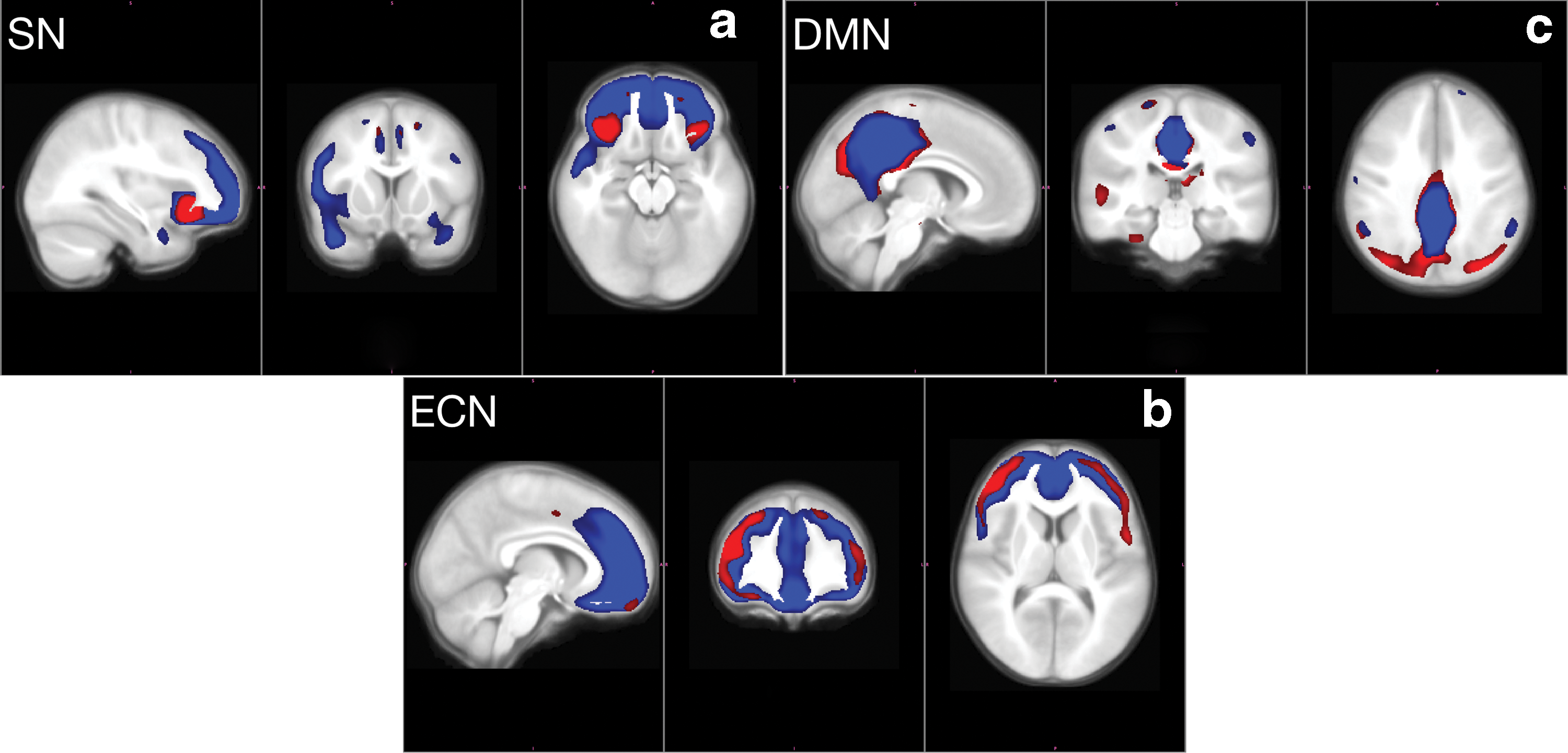
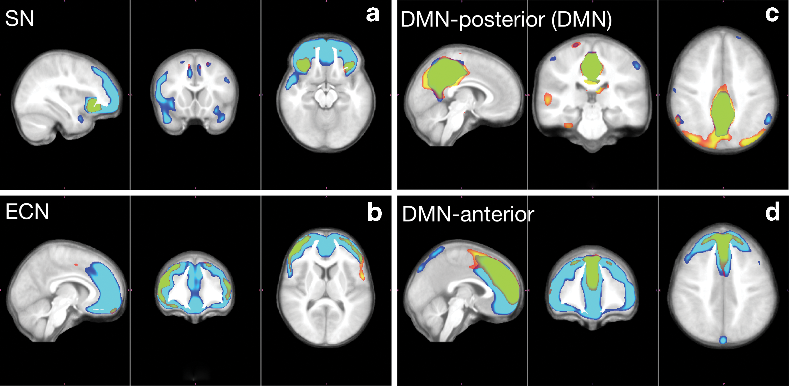
For each diagnostic group and each seed ROI, we obtain the set of regions covarying with the seed ROI, following the process described in the Structural correlation graphs section. The structural covariance maps corresponding to the seed ROI are shown in Figure 1a–c. Further comparisons in Figure 2a–d show that the maps for two diagnostic groups do not completely overlap. Some regions present in the map for the control group are absent in the map for the autism group. Conversely, some regions are present only in the map for the autism group, but not in the map for the control group. Table 1 lists the number of regions present in controls, but not in autism; in autism, but not in controls; and in both; as well as in either autism or control. A network-specific set of ROIs is given by the union of all regions covarying with the corresponding seed ROI in either the autism group map or the control group map.
Structural covariance maps. (a) Structural covariance map with seed in right fronto-insular cortex anchoring SN. (b) Structural covariance map with seed in right dorsolateral prefrontal cortex anchoring ECN. (c) Structural covariance map with seed in right posterior cingulate cortex anchoring the default mode network. In all three subfigures, red represents the structural covariance map for the autism group and blue represents the structural covariance map for TDCs. ECN, executive control network; SN, salience network; TDC, typically developing control. Color images are available online.
Structural covariance maps further illustrated. (a) Structural covariance map with seed in right fronto-insular cortex anchoring SN. (b) Structural covariance map with seed in right dorsolateral prefrontal cortex anchoring ECN. (c) Structural covariance map with seed in right posterior cingulate cortex anchoring the default mode network. (d) Structural covariance map with seed in anterior part anchoring the default mode network. In all four subfigures, structural covariance maps are further illustrated here with red to yellow (autism) and dark blue to light blue (control) look-up tables. Color gradation indicates increasing statistical significance. Overlapping regions among autism and control groups are highlighted in green (c) and (d). Our data consist of subjects with an average age of about 13 years. The underlying structure of the default mode network is not fully developed at this age. We include two maps with different seeds to illustrate that the posterior part (c) is not yet integrated with the anterior part (d). In our analysis, we use the posterior covariance map (c), which corresponds to the most common seed for the default mode network in adults. Color images are available online.
Number of Regions of Interest Identified from Structural Covariance Magnetic Resonance Imaging for Given Seed Regions
Seed (SCG)
Controls only
Autism only
Both
Either
R PCC (DMN-SCG)
9
21
9
39
R FI (SN-SCG)
21
1
10
32
R DLPC (ECN-SCG)
22
5
12
39
For each network-specific SCG, the table shows the number of regions identified from the structural covariance map in controls only, in autism only, in both autism and controls, and in either autism or controls. The first column lists the seed along with the name of corresponding SCG in parentheses.
DMN, default mode network; ECN, executive control network; R DLPC, right dorsolateral prefrontal cortex; R FI, right fronto-insular cortex; R PCC, right posterior cingulate cortex; SCG, structural correlation graph; SN, salience network.
Thus, we have one Global set of ROIs and three network-specific sets of regions. For each set of ROIs, we compute the group-level SCGs and perform the random permutation test as described in the Permutation test section. We perform one million permutations in case of network-specific SCGs and 10,000 permutations in case of the Global-SCG (due to computational constraints). We also perform the bootstrap test as described in the Bootstrap test section with one million bootstrap samples in case of network SCGs and 10,000 in case of the Global-SCG.
Type I error rate for permutation test
The number of permutations in an exact permutation test depends on the number of subjects in the sample. Our random permutation test closely approximates this exact test. However, it should be noted that the test does not take into account the number of ROIs. To check whether our test is robust to increasing number of ROIs, we have implemented the following simulation.
We generate two \documentclass{aastex}\usepackage{amsbsy}\usepackage{amsfonts}\usepackage{amssymb}\usepackage{bm}\usepackage{mathrsfs}\usepackage{pifont}\usepackage{stmaryrd}\usepackage{textcomp}\usepackage{portland, xspace}\usepackage{amsmath, amsxtra}\usepackage{upgreek}\pagestyle{empty}\DeclareMathSizes{10}{9}{7}{6}\begin{document}$$m \times n$$ \end{document} data matrices (m is the number of subjects and n is the number of ROIs), where each element is randomly generated from a standard normal distribution so that both the samples (data matrices) come from the same underlying distribution. We compute SCGs from these data matrices and perform the random permutation test as described in the Statistical inference section. Since the underlying distribution of samples is the same, rejecting the null hypothesis would be a type I error.
We keep the number of subjects, \documentclass{aastex}\usepackage{amsbsy}\usepackage{amsfonts}\usepackage{amssymb}\usepackage{bm}\usepackage{mathrsfs}\usepackage{pifont}\usepackage{stmaryrd}\usepackage{textcomp}\usepackage{portland, xspace}\usepackage{amsmath, amsxtra}\usepackage{upgreek}\pagestyle{empty}\DeclareMathSizes{10}{9}{7}{6}\begin{document}$$m \; = \;$$ \end{document}100, fixed through the whole simulation. Then, we set the number of ROIs, n = 10, 50, 100, 500, and 1000, respectively, and for each value of n, we perform 100 random permutation tests as described in the previous paragraph to find the proportion of tests resulting in type I error. Table 2 shows the findings. At the 0.05 level of significance, our permutation test is more conservative, meaning it is much less likely to get false positives.
Type I Error Rate for Increasing Number of Regions of Interest
No. of ROIs
10
50
100
500
1000
Type I error rate
0.01
0.02
0.03
0.05
0.03
For number of ROIs = 10, 50, 100, 500, and 1000, the table lists the rate of type I errors (false positives) obtained from the simulation described in the Type I error rate for permutation test section.
ROI, region of interest.
Results
We apply both the random permutation test and bootstrap test to compare SCGs across groups of subjects with autism and TDC subjects. We begin by comparing global SCGs comprising 7266 gray matter regions in the preprocessed images. Then, for a closer analysis, we compare the SCGs generated with seed ROIs anchoring the three ICNs (SN, ECN, and DMN) referred to as SN-SCG, ECN-SCG, and DMN-SCG. These are much smaller SCGs, comprising 32, 39, and 39 ROIs, respectively (Table 1). Recall that structural covariance maps for the autism and control groups overlap in very few regions. We construct and compare SCGs derived from sets of regions that are present either in controls or in autism.
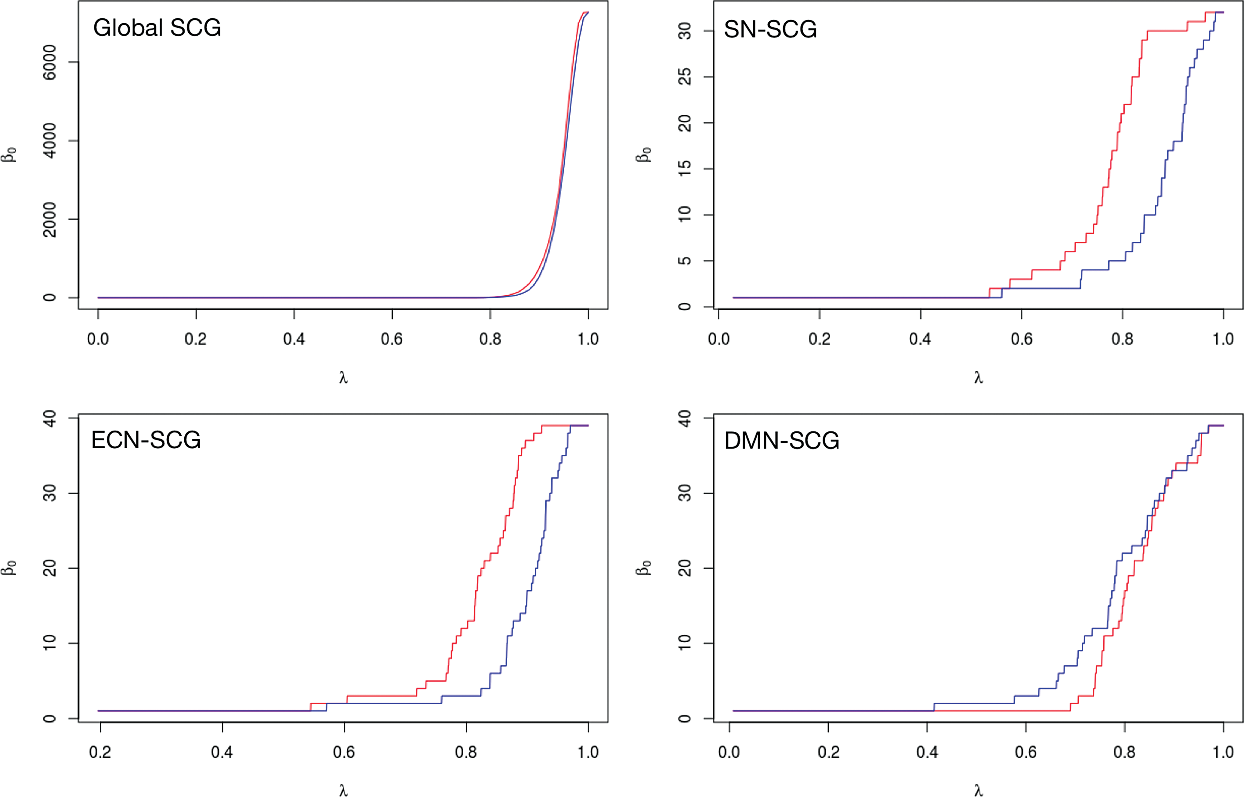
The \documentclass{aastex}\usepackage{amsbsy}\usepackage{amsfonts}\usepackage{amssymb}\usepackage{bm}\usepackage{mathrsfs}\usepackage{pifont}\usepackage{stmaryrd}\usepackage{textcomp}\usepackage{portland, xspace}\usepackage{amsmath, amsxtra}\usepackage{upgreek}\pagestyle{empty}\DeclareMathSizes{10}{9}{7}{6}\begin{document}$${ \beta _0}$$ \end{document} curves corresponding to global SCGs and seed-specific SCGs are shown in Figure 3a–d. Table 3 lists estimated p-values obtained from random permutation tests along with standard errors in the estimation. Note that the number of permutations is sufficiently large in each case so that the estimation standard errors are small and not likely to affect outcomes of the permutation tests. Table 4 lists p-values obtained from the bootstrap test. Note that conclusions from both tests are comparable at the 0.05 level of significance. By combining topological data analysis with statistical inference, our results provide evidence of statistically significant network-specific structural abnormalities in autism SN-SCGs.
β0 curves. Top left: β0 curves corresponding to whole-brain SCGs. Top right: β0 curves corresponding to SCGs derived from SNs. Bottom left: β0 curves corresponding to SCGs derived from ECNs. Bottom right: β0 curves corresponding to SCGs derived from default mode networks. In all four subfigures, red represents the curve for the autism group and blue represents the curve for the control group. SCG, structural correlation graph. Color images are available online.
Estimated p-Values for Random Permutation Tests on Structural Correlation Graphs and Corresponding Standard Errors
Global-SCG
DMN-SCG
SN-SCG
ECN-SCG
p-Value estimate
0.3985
0.3658
0.00614
0.1118
Standard error
0.004895
0.000481
0.000078
0.000315
For each of the SCGs considered in our analysis, the table gives estimated p-values from the random permutation test described in the Permutation test section. Only significant p-value was obtained for the SCG derived from the SN, which is highlighted in bold face. The second row of the table gives estimated error rates for p-values.
p-Values for Bootstrap Test on Structural Correlation Graphs
Global-SCG
DMN-SCG
SN-SCG
ECN-SCG
p-Value
0.3685
0.3970
0.0073
0.0890
For each of the SCGs considered in our analysis, the table gives estimated p-values from the bootstrap test described in the Bootstrap test section. Only significant (≤0.05) p-value was obtained for SCG derived from the SN, which is highlighted in bold face.
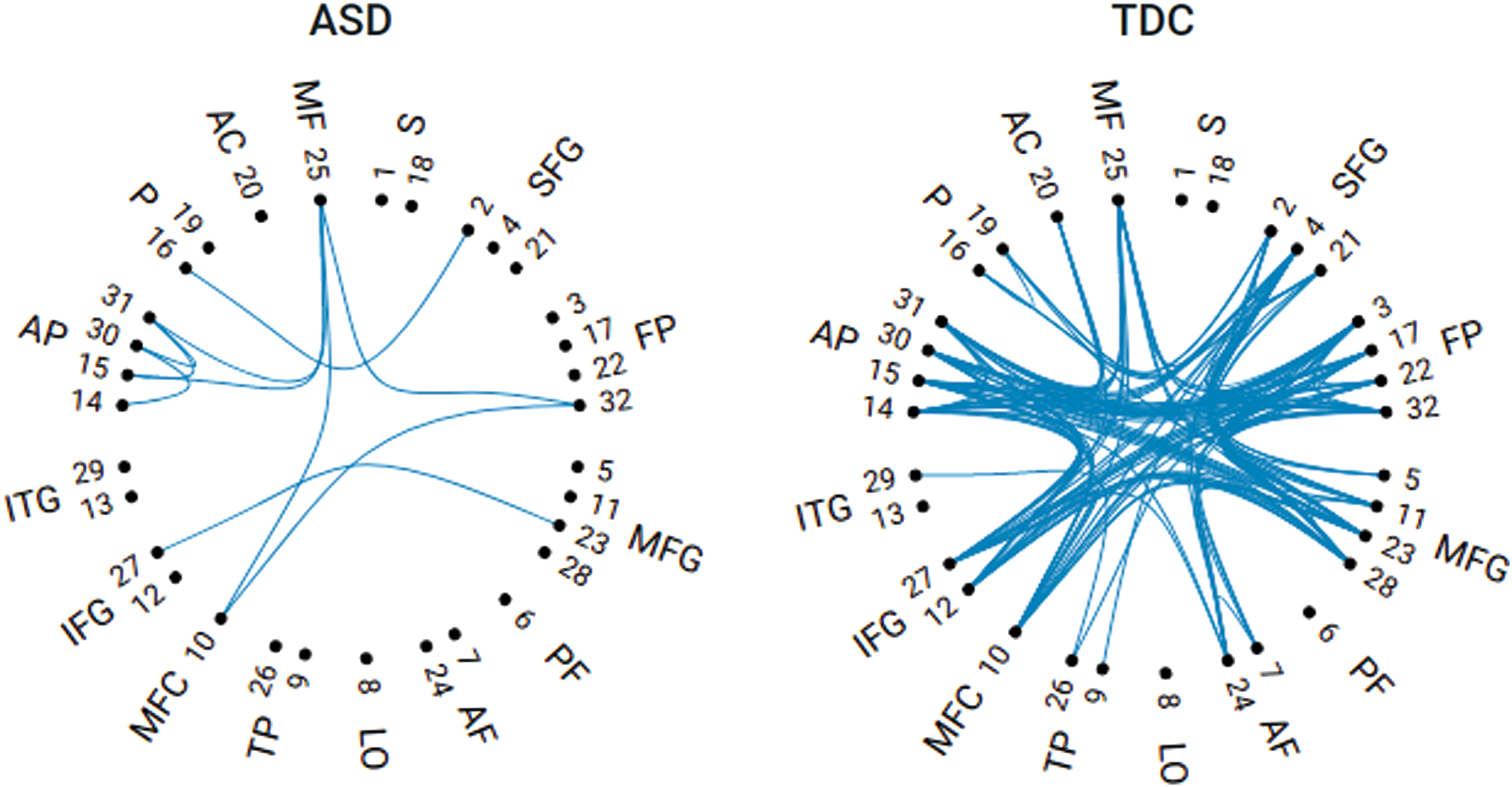
Figure 4 shows a comparative visualization of the two SN-SCGs that correspond to ASD and TDC groups, respectively, at the threshold \documentclass{aastex}\usepackage{amsbsy}\usepackage{amsfonts}\usepackage{amssymb}\usepackage{bm}\usepackage{mathrsfs}\usepackage{pifont}\usepackage{stmaryrd}\usepackage{textcomp}\usepackage{portland, xspace}\usepackage{amsmath, amsxtra}\usepackage{upgreek}\pagestyle{empty}\DeclareMathSizes{10}{9}{7}{6}\begin{document}$$\lambda = 0.8174$$ \end{document}. This is the threshold at which the gap between the corresponding \documentclass{aastex}\usepackage{amsbsy}\usepackage{amsfonts}\usepackage{amssymb}\usepackage{bm}\usepackage{mathrsfs}\usepackage{pifont}\usepackage{stmaryrd}\usepackage{textcomp}\usepackage{portland, xspace}\usepackage{amsmath, amsxtra}\usepackage{upgreek}\pagestyle{empty}\DeclareMathSizes{10}{9}{7}{6}\begin{document}$${ \beta _0}$$ \end{document} curves is the largest (\documentclass{aastex}\usepackage{amsbsy}\usepackage{amsfonts}\usepackage{amssymb}\usepackage{bm}\usepackage{mathrsfs}\usepackage{pifont}\usepackage{stmaryrd}\usepackage{textcomp}\usepackage{portland, xspace}\usepackage{amsmath, amsxtra}\usepackage{upgreek}\pagestyle{empty}\DeclareMathSizes{10}{9}{7}{6}\begin{document}$${D_q} = 21$$ \end{document}, with \documentclass{aastex}\usepackage{amsbsy}\usepackage{amsfonts}\usepackage{amssymb}\usepackage{bm}\usepackage{mathrsfs}\usepackage{pifont}\usepackage{stmaryrd}\usepackage{textcomp}\usepackage{portland, xspace}\usepackage{amsmath, amsxtra}\usepackage{upgreek}\pagestyle{empty}\DeclareMathSizes{10}{9}{7}{6}\begin{document}$${ \beta _0}$$ \end{document} being 6 and 27 for ASD and TDCs, respectively).
Comparative visualization of SN-SCG. SN-SCG at threshold \documentclass{aastex}\usepackage{amsbsy}\usepackage{amsfonts}\usepackage{amssymb}\usepackage{bm}\usepackage{mathrsfs}\usepackage{pifont}\usepackage{stmaryrd}\usepackage{textcomp}\usepackage{portland, xspace}\usepackage{amsmath, amsxtra}\usepackage{upgreek}\pagestyle{empty}\DeclareMathSizes{10}{9}{7}{6}\begin{document}$$\lambda = 0.8174$$ \end{document}, which corresponds to \documentclass{aastex}\usepackage{amsbsy}\usepackage{amsfonts}\usepackage{amssymb}\usepackage{bm}\usepackage{mathrsfs}\usepackage{pifont}\usepackage{stmaryrd}\usepackage{textcomp}\usepackage{portland, xspace}\usepackage{amsmath, amsxtra}\usepackage{upgreek}\pagestyle{empty}\DeclareMathSizes{10}{9}{7}{6}\begin{document}$$D_q^*$$ \end{document} for both ASD (left) and TDC (right) groups. ROIs (4-mm spheres) are grouped by anatomical regions they are placed in as follows: S, SMA; SFG, superior frontal gyrus; FP, frontal pole; MFG, middle frontal gyrus; PF, postfusiform; AF, anterior fronto-insular; LO, lateral occipital; TP, temporal pole; MFC, medial frontal cortex; IFG, inferior frontal gyrus; ITG, inferior temporal gyrus; AP, anterior paracingulate; P, paracingulate; AC, anterior cingulate; MF, medial frontal (ventro-medial prefrontal cortex or VMPFC). Image courtesy of Yiliang Shi, University of Utah. Color images are available online.
The visualization shows that gray matter densities are much less correlated across ASD subjects compared with TDC subjects. The most likely reason behind these differences is that there is more idiosyncrasy in the autism cohort, in which regions show greater or lesser cortical thickness or subtle differences in the positions of gyri or sulci. There is a growing sense that this idiosyncrasy might be the most reliable difference in autism, meaning that each ASD case is unique, different from group mean values in some way.
Conclusion and Discussion
Exact statistical inference
In an earlier effort, Palande and colleagues (2017) used an exact statistical inference method, originally proposed by Chung and colleagues (2017), to test the significance of differences in the connectivity of SCGs. Chung and colleagues (2017; theorem 2) have given a combinatorial construction of an exact p-value along with an expression for the asymptotic p-value. Such a construction is the same as the combinatorial construction of the two-sample Kolmogorov–Smirnov test and uses the fact that \documentclass{aastex}\usepackage{amsbsy}\usepackage{amsfonts}\usepackage{amssymb}\usepackage{bm}\usepackage{mathrsfs}\usepackage{pifont}\usepackage{stmaryrd}\usepackage{textcomp}\usepackage{portland, xspace}\usepackage{amsmath, amsxtra}\usepackage{upgreek}\pagestyle{empty}\DeclareMathSizes{10}{9}{7}{6}\begin{document}$${ \beta _0}$$ \end{document} sequences are monotonic increasing sequences.
In this study, we discuss why this exact inference method is, in fact, not appropriate in our setting. Recall that our data are represented as two \documentclass{aastex}\usepackage{amsbsy}\usepackage{amsfonts}\usepackage{amssymb}\usepackage{bm}\usepackage{mathrsfs}\usepackage{pifont}\usepackage{stmaryrd}\usepackage{textcomp}\usepackage{portland, xspace}\usepackage{amsmath, amsxtra}\usepackage{upgreek}\pagestyle{empty}\DeclareMathSizes{10}{9}{7}{6}\begin{document}$$m \times n$$ \end{document} matrices, m being the number of ASD or TDC subjects and n being the number of ROIs.
In the study by Chung and colleagues (2017; theorem 2), the p-value for the exact inference obtained combinatorially only depends on n, the number of connected components (i.e., the number of ROIs). Therefore, the p-value computation by Chung and colleagues (2017; theorem 2) is independent of the sample size. However, for a hypothesis test of group differences, we would expect p-values to be dependent on the sample size, therefore the computation by Chung and colleagues (2017; theorem 2) is not applicable in our setting.
Applying the theorem (Chung et al., 2017; theorem 2) directly in our setting would imply an enumeration of permutations over ROIs with \documentclass{aastex}\usepackage{amsbsy}\usepackage{amsfonts}\usepackage{amssymb}\usepackage{bm}\usepackage{mathrsfs}\usepackage{pifont}\usepackage{stmaryrd}\usepackage{textcomp}\usepackage{portland, xspace}\usepackage{amsmath, amsxtra}\usepackage{upgreek}\pagestyle{empty}\DeclareMathSizes{10}{9}{7}{6}\begin{document}$$\left( { \begin{matrix} {2n} \\ n \\ \end{matrix} }\right)$$ \end{document} possibilities. Our standard permutation test, on the other hand, has \documentclass{aastex}\usepackage{amsbsy}\usepackage{amsfonts}\usepackage{amssymb}\usepackage{bm}\usepackage{mathrsfs}\usepackage{pifont}\usepackage{stmaryrd}\usepackage{textcomp}\usepackage{portland, xspace}\usepackage{amsmath, amsxtra}\usepackage{upgreek}\pagestyle{empty}\DeclareMathSizes{10}{9}{7}{6}\begin{document}$$\left( { \begin{matrix} {2m} \\ m \\ \end{matrix} } \right )$$ \end{document} possible permutations since each sample consists of m subjects. In our experiment, the set of ROIs for each SCG is selected because of their high covariance with a particular seed region. These ROIs are meant to represent specific attributes of the ASD and TDC populations. Permuting ROIs would result in sets of ROIs that do not represent either of these populations. Again, the exact inference procedure (Chung et al., 2017; theorem 2) is clearly unrelated to the standard permutation test in our setting.
In summary, the exact inference method proposed by Chung and colleagues (2017) is not applicable here to make inferences about population differences between the ASD and TD subjects.
Highlights, limitations, and future directions
Similar covariance of gray matter density across a population of individuals is thought to be mediated by shared genetic or developmental factors (Zielinski et al., 2012). Structural covariance maps help us identify brain regions highly covarying with a specific seed region. These maps not only exhibit similar architecture to more familiar ICNs derived from functional MRI images (Fox and Raichle, 2007) but also exhibit differences in architecture, with extensive regions of the frontal lobe showing greater alignment with the SN and ECN rather than with the DMN (Zielinski et al., 2010). These differences suggest that while these frontal lobe regions may show greater synchrony with DMN regions such as posterior cingulate cortex and temporoparietal junction, the developmental influences across subjects may be more related to changes in brain attentional networks.
Zielinski and colleagues (2012) have performed direct comparisons of structural covariance maps. The regions in these maps are assigned significance measures based on their covariance with respect to the specified seed region. Using these maps, Zielinski and colleagues have shown the existence of multidimensional structure–function relationships. Our work helps summarize these relationships using a more robust, topological, data analysis model. SCGs encode all pairwise associations among the ROIs, where the extent of an association is measured by the magnitude of correlations across subjects. Our experiments provide evidence of statistically significant differences in the zero-dimensional topological features of SCGs derived from SN (SN-SCGs).
Our results confirm the significant differences in structural covariance in autism, therefore being consistent with the findings of Zielinski and colleagues. The most striking findings in our results show decreased structural covariance among individuals with autism in the integration of frontal lobe regions with SN hubs in the fronto-insula. Our findings of decreased integration of salience and executive networks, with increased integration of default regions within the frontal lobe, align with results investigating functionally defined ICNs (Abbott et al., 2016) and suggest that shared developmental influences may underlie the particular specificity of SN connectivity abnormalities in autism (Uddin et al., 2013).
The DMN has also been associated with atypical connectivity in autism (Anderson et al., 2011; Assaf et al., 2010; Chen et al., 2015; Lynch et al., 2013). Specifically, decreased within-network integration and increased between-network connectivity for the DMN have been reported in autism; see Padmanabhan and colleagues (2017). The increased structural covariance between the posterior cingulate cortex and default regions, but decreased anterior DMN integration, may suggest that DMN connectivity differences in autism may be related to altered development of frontal lobe components of the network with more idiosyncratic development of frontal network architecture in autism.
Our experiments fail to capture any statistically significant differences in the topology of SCGs derived from DMN. It is possible that the aforementioned idiosyncratic development results in more complex topological differences that are not captured by the pairwise interactions between ROIs. The \documentclass{aastex}\usepackage{amsbsy}\usepackage{amsfonts}\usepackage{amssymb}\usepackage{bm}\usepackage{mathrsfs}\usepackage{pifont}\usepackage{stmaryrd}\usepackage{textcomp}\usepackage{portland, xspace}\usepackage{amsmath, amsxtra}\usepackage{upgreek}\pagestyle{empty}\DeclareMathSizes{10}{9}{7}{6}\begin{document}$${ \beta _0}$$ \end{document} curves only encode zero-order topological features that correspond to the evolution of the number of connected components. Analyzing three-way or four-way interactions between ROIs, capturing higher-order topological features such as tunnels and voids, and focusing on specific nodes and edges directly involved in merging components in the graph filtration may provide further insights into differences in DMN architecture.
Last, it should be noted that the SCGs reported here are abstract networks and do not represent physical connectivity between the regions. This limits the interpretability of our results to some extent, and deeper analysis is needed to quantify and better interpret the differences suggested by the statistical inference.
Footnotes
Acknowledgments
This work was supported, in part, by an NSF grant IIS-1513616 and NIH grants R01EB022876, K08MH100609, and R01MH080826. was generated using a comparative visualization tool developed by Yiliang Shi, University of Utah.
Author Disclosure Statement
No competing financial interests exist.
References
1.
AbbottAE, NairA, KeownCL, DatkoM, JahediA, FishmanI, MullerRA. 2016. Patterns of atypical functional connectivity and behavioral links in autism differ between default, salience, and executive networks. Cereb Cortex, 26:4034–4045.
2.
AltayeM, HollandSK, WilkeM, GaserC. 2008. Infant brain probability templates for MRI segmentation and normalization. Neuroimage, 43:721–730.
3.
AndersonJS, NielsenJA, FroehlichAL, DubrayMB, DruzgalTJ, CarielloAN, et al.2011. Functional connectivity magnetic resonance imaging classification of autism. Brain, 134:3742–3754.
4.
AssafM, JagannathanK, CalhounVD, MillerL, StevensMC, SahlR, et al.2010. Abnormal functional connectivity of default mode sub-networks in autism spectrum disorder patients. Neuroimage, 53:247–256.
5.
BullmoreE, SpornsO. 2009. Complex brain networks: graph theoretical analysis of structural and functional systems. Nat Rev Neurosci, 10:186–198.
6.
ChenCP, KeownCL, JahediA, NairA, PiegerME, BaileyBA, MullerRA. 2015. Diagnostic classification of intrinsic functional connectivity highlights somatosensory, default mode, and visual regions in autism. Neuroimage Clin, 8:238–245.
7.
ChungMK, Villalta-GilV, LeeH, RathouzPJ, LaheyBB, ZaldDH. 2017. Exact topological inference for paired brain networks via persistent homology. Inf Process Med Imaging, 2017:299–231.
8.
CourchesneE, PierceK, SchumannCM, RedcayE, BuckwalterJA, KennedyDP, MorganJ. 2007. Mapping early brain development in autism. Neuron, 56:399–413.
FairDA, CohenAL, DosenbachNUF, ChurchJA, MiezinFM, BarchDM, et al.2008. The maturing architecture of the brain's default network. Proc Natl Acad Sci, 105:4028–4032.
11.
FoxMD, RaichleME. 2007. Spontaneous fluctuations in brain activity observed with functional magnetic resonance imaging. Nat Rev Neurosci, 8:700–711.
12.
FoxMD, SnyderAZ, VincentJL, CorbettaM, Van EssenDC, RaichleME. 2005. The human brain is intrinsically organized into dynamic, anticorrelated functional networks. Proc Natl Acad Sci U S A, 102:9673–9678.
13.
LeeH, KangH, ChungMK, KimBN, LeeDS. 2012. Persistent brain network homology from the perspective of dendrogram. IEEE Trans Med Imag, 31:2267–2277.
14.
LynchCJ, UddinLQ, SupekarK, KhouzamA, PhillipsJ, MenonV. 2013. Default mode network in childhood autism: posteromedial cortex heterogeneity and relationship with social deficits. Biol Psychiatry, 74:212–219.
15.
MinkovaL, EickhoffSB, AbdulkadirA, KallerCP, PeterJ, SchellerE, et al.2016. Large-scale brain network abnormalities in Huntington's disease revealed by structural covariance. Hum Brain Mapp, 37:67–80.
16.
MontembeaultM, RouleauI, ProvostJ-S, BrambatiSM. 2016. Altered gray matter structural covariance networks in early stages of Alzheimer's disease. Cereb Cortex, 26:2650.
17.
PadmanabhanA, LynchCJ, SchaerM, MenonV. 2017. The default mode network in autism. Biol Psychiatry Cogn Neurosci Neuroimaging, 2:476–486.
18.
PalandeS, JoseV, ZielinskiB, AndersonJ, FletcherPT, WangB. 2017. Revisiting abnormalities in brain network architecture underlying autism using topology-inspired statistical inference. In: WuG, LaurientiP, BonilhaL, and MunsellB (eds.) Connectomics in NeuroImaging (CNI), Lecture Notes in Computer Science, volume 10511. Cham: Springer; pp. 98–107.
19.
SchumannCM, BlossCS, BarnesCC, WidemanGM, CarperRA, AkshoomoffN, et al.2010. Longitudinal magnetic resonance imaging study of cortical development through early childhood in autism. J Neurosci, 30:4419–4427.
SeeleyWW, MenonV, SchatzbergAF, KellerJ, GloverGH, KennaH, et al.2007. Dissociable intrinsic connectivity networks for salience processing and executive control. J Neurosci, 27:2349–2356.
22.
StiglerKA, McDonaldBC, AnandA, SaykinAJ, McDougleCJ. 2011. Structural and functional magnetic resonance imaging of autism spectrum disorders. Brain Res, 1380:146–161.
23.
UddinLQ, SupekarK, LynchCJ, KhouzamA, PhillipsJ, FeinsteinC, et al.2013. Salience network-based classification and prediction of symptom severity in children with autism. JAMA Psychiatry, 70:869–879.
24.
WilkeM, HollandSK, AltayeM, GaserC. 2008. Template-OMatic: a toolbox for creating customized pediatric templates. Neuroimage, 41:903–913.
25.
ZielinskiBA, AndersonJS, FroehlichAL, PriggeMBD, NielsenJA, CooperriderJR, et al.2012. scMRI reveals large-scale brain network abnormalities in autism. PLoS One, 7:1–14.
26.
ZielinskiBA, GennatasED, ZhouJ, SeeleyWW. 2010. Network-level structural covariance in the developing brain. Proc Natl Acad Sci, 107:18191–18196.
27.
ZielinskiBA, PriggeMBD, NielsenJA, FroehlichAL, AbildskovTJ, AndersonJS, et al.2014. Longitudinal changes in cortical thickness in autism and typical development. Brain, 137:1799–1812.