Dynamic Functional Network Connectivity in Schizophrenia with Magnetoencephalography and Functional Magnetic Resonance Imaging: Do Different Timescales Tell a Different Story?

Abstract

The importance of how brain networks function together to create brain states has become increasingly recognized. Therefore, an investigation of eyes-open resting-state dynamic functional network connectivity (dFNC) of healthy controls (HC) versus that of schizophrenia patients (SP) via both functional magnetic resonance imaging (fMRI) and a novel magnetoencephalography (MEG) pipeline was completed. The fMRI analysis used a spatial independent component analysis (ICA) to determine the networks on which the dFNC was based. The MEG analysis utilized a source space activity estimate (minimum norm estimate [MNE]/dynamic statistical parametric mapping [dSPM]) whose result was the input to a spatial ICA, on which the networks of the MEG dFNC were based. We found that dFNC measures reveal significant differences between HC and SP, which depended on the imaging modality. Consistent with previous findings, a dFNC analysis predicated on fMRI data revealed HC and SP remain in different overall brain states (defined by a k-means clustering of network correlations) for significantly different periods of time, with SP spending less time in a highly connected state. The MEG dFNC, in contrast, revealed group differences in more global statistics: SP changed between meta-states (k-means cluster states that are allowed to overlap in time) significantly more often and to states that were more different, relative to HC. MEG dFNC also revealed a highly connected state where a significant difference was observed in interindividual variability, with greater variability among SP. Overall, our results show that fMRI and MEG reveal between-group functional connectivity differences in distinct ways, highlighting the utility of using each of the modalities individually, or potentially a combination of modalities, to better inform our understanding of disorders such as schizophrenia.

Introduction

Noninvasive neuroimaging is currently available in a number of modalities, including functional magnetic resonance imaging (fMRI) with its excellent spatial resolution and magnetoencephalography (MEG) with its excellent temporal resolution. Harnessing and/or combining the strengths these modalities offer are of great interest in both healthy and patient populations, which can aid in informing the classification of patient populations, identification of new treatment targets, and/or potential treatment success. One of the main goals of multimodal imaging is to provide clinicians with biomarkers to assist with producing a diagnosis with increased confidence and predicting a long-term prognosis for each new patient.

Importantly, theoretical and experimental evidence implies that the biological signals detected by both fMRI and MEG originate from postsynaptic currents, although in a complex manner potentially variable by brain region (Ahonen et al., 1993; Conner et al., 2011; Hamalainen et al., 1993; Harvey et al., 2013; Zhu et al., 2009), indicating that the combination and/or comparison of MEG and fMRI make theoretical sense (Hall et al., 2014). Although the exact relationship and influence of particular frequency bands remain an open question, the relationship between blood oxygen-level dependent (BOLD) signal and electrophysiological activation has been shown for a variety of task activations in gamma band (Kunii et al., 2013; Lachaux et al., 2007; Niessing, et al., 2005; Scheeringa et al., 2011; Zaehle et al., 2009), and it has been shown that in the resting state the direction (positive or negative) of electroencephalography (EEG)-BOLD signal correlations varies across brain regions and frequency bands, with lower as well as higher frequency brain oscillations linked to neurovascular processes.

Of particular relevance here, it was found that low-frequency oscillations (<20 Hz), and not gamma activity, predominantly contributed to interareal BOLD correlations (Wang et al., 2012). The authors report that these low-frequency oscillations also influenced local processing by modulating gamma activity within individual areas, and suggest that such cross-frequency coupling links local BOLD signals to correlations across distributed networks. In addition, results from Bridwell et al. (2013) characterized brain networks spatially and spectrally, revealing that positive and negative associations appear within overlapping regions of the EEG frequency spectrum. That is, positive associations were primarily present within the lower (delta and theta) and higher (upper beta and lower gamma) spectral regions, sometimes within the same brain regions as measured by fMRI.

Finally, it has been shown that even though the two modalities (fMRI and MEG/EEG) may exhibit activity in similar spatial locations, the functional pattern of this activity may differ in a complex manner, suggesting that each modality may be tuned to different aspects of neuronal activity (Muthukumaraswamy and Singh, 2008). Taken together these findings imply a complex relationship between neuronal activation and neurovascular coupling as measured by the BOLD signal, and suggest that all frequency bands contained in the MEG/EEG signal are potentially of interest when studying patient populations.

It has been shown in fMRI by Abrol et al. (2016) that multiple discrete, reoccurring connectivity states arise during rest, and that subjects tend to remain in one connectivity state for relatively long periods of time before transitioning to another. Other researchers observed how brain regions spontaneously changed their “module affiliations” (i.e., network connectivity) on a temporal scale of seconds, which could not be simply attributable to head motion or other errors (Liao, et al., 2017; Vergara et al., 2017). Similarly, in electrophysiological data, it has been shown that sensor space “microstates” arise and change on the order of hundreds of milliseconds (Baker et al., 2014; Khanna et al., 2015; Van de Ville, et al., 2010) and vary between disorders dependent on which network a microstate correlated with (e.g., a microstate that correlated with the frontoparietal network was impaired in schizophrenia) (Nishida et al., 2013). Patients with schizophrenia (SP) have been investigated in this manner by others as well, with SP experiencing particular microstates more often and also experiencing briefer microstates than did healthy controls (HC) (review: Rieger et al., 2016).

One way to summarize the recurring connectivity states described above is via a functional network connectivity (FNC) analysis, which may be defined as the way in which sets of brain areas (networks) work together over time to produce different brain states, represented by statistical associations between network timecourses without regard to the spatial proximity of the regions to one another. An increasing body of literature suggests that neural oscillations perform a key role in binding separate brain regions together and promoting information transfer between distant brain areas (Buzsáki and Draguhn, 2004; Engel and Singer, 2001; Roopun et al., 2008). FNC has become an important metric for the study of how this naturally occurs (Allen et al., 2014; Calhoun, et al., 2014; Jafri et al., 2008). Furthermore, connectivity between brain regions is now generally accepted as being key to healthy brain function (Hall et al., 2014).

Clearly, the temporal, as well as the spatial, properties of these networks are of importance to our understanding of brain function, and it is probable that the definition of a network may vary on different timescales (Erhardt et al., 2011a,b). Over the past decade, FNC has most often been investigated within the resting state (i.e., in the absence of a defined task) using fMRI (Allen et al., 2011; Biswal et al., 1995; Biswal, 2012) and, to a lesser extent, electrophysiological methods, MEG and EEG (Allen et al., 2018; Brookes et al., 2011a, b; Meier et al., 2016; Nugent et al., 2017), in diverse populations, including schizophrenia, depression, bipolar disorder, and in aging (Alamian, et al., 2017; Cetin et al., 2016; Dong, et al., 2018; Du, et al., 2016; Fox et al., 2017; Houck et al., 2017; Madden, 2017; Nashiro et al., 2017; Roiser et al., 2016; Wu et al., 2017).

To date, FNC has most often been assessed as a static feature of the data, inferred from the overall (arbitrary) duration of the scan. However, there is no a priori reason to assume that in the resting brain, network correlations are static; indeed, based on the known rapid dynamics of brain oscillations, it may instead be expected that connections across networks change over time, even during a brief resting scan, as subjects experience different mental and emotional states (Miller et al., 2014, 2016).

The logical extension of FNC that looks at how states vary over small time “windows” to capture networks on a finer temporal scale has been termed dynamic functional network connectivity (dFNC). dFNC has also been investigated in resting-state fMRI (Miller, et al., 2014; Sakoğlu et al., 2010) and in diagnostic groups such as schizophrenia patients (Damaraju et al., 2014; Miller, et al., 2014), where for schizophrenia patients in an eyes-closed resting scan it has been shown that there is a reduction in fluidity, or dynamism, in their ability to move from state to state. Importantly, the dFNC spatial patterns of intrasubject dynamic variability have been shown to largely overlap with that of intersubject variability, both of which were highly reproducible across repeated scanning sessions (Abrol et al., 2016). dFNC has therefore been established as a useful tool for both investigating changing brain states and for determining how these states vary between patient populations.

In this study, we present a dFNC analysis using MEG and fMRI eyes-open resting scans collected from the same sample of HC and schizophrenia patients, and indicate where we find overlap and differences between the results from the different modalities. We discuss possible reasons for these results, including careful selection of analysis parameters and scan length, particularly for the MEG data analysis where this has not been extensively studied previously. For the dFNC of fMRI data, we follow an established pipeline (Calhoun et al., 2014; Miller et al., 2014).

For the MEG data analysis, we describe the creation of a novel pipeline that includes a source space analysis (MNE/dSPM, i.e., dynamic statistical parametric mapping from within minimum norm estimate software) as input to a spatial independent component analysis (ICA) as the basis for the dFNC. We argue that using components calculated in such a way helps mitigate the “signal leakage” problem for MEG source space-based analyses as leakage manifests in the spatial maps, but the network connectivity patterns (CP) are preserved (Houck, et al., 2017).

Finally, we investigate group differences between HC and schizophrenia patients for both methods. We expect that SP will spend less time in highly connected brain states. We further hypothesize that for both fMRI and MEG analysis SP will show a reduction in global meta-state statistic values that measure how and when individuals move between states at a global level, relative to HC (i.e., we will see a “reduced dynamism” for SP).

Materials and Methods

Participants

Briefly, this investigation combined existing data (Aine et al., 2017) from 46 schizophrenia patients and 45 HC from whom informed consent was obtained according to institutional guidelines at the University of New Mexico Human Research Protections Office (HRPO). All participants were compensated for their participation. Patients with a diagnosis of schizophrenia or schizoaffective disorder were invited to participate. Each patient completed the Structured Clinical Interview for DSM-IV Axis I Disorders (First et al., 1997) for diagnostic confirmation and evaluation of comorbidities. Exclusion criteria included history of neurological disorders, mental retardation, substance abuse, or clinical instability. Patients were treated with a variety of antipsychotic medications, and therefore, doses of antipsychotic medications were converted to olanzapine equivalents (Table 1) (Gardner et al., 2010).

Table 1.

Independent Component Analysis Component Numbers and Anatomical Locations

MEG ICA component No.	Component ID
1	Auditory (Left)
2	Posterior cingulate (Bilateral)
3	Lateral occipital (Right)
4	Parahippocampus (Bilateral)
5	Superior frontal (Right)
6	Precuneus (Right)
7	Medial orbital frontal (Bilateral)
8	Supramarginal (Left)
9	Temporal pole (Right)
10	Insula (Right)
11	Visual (Left)
12	Precuneus (Left)
13	Paracentral (Right)
14	IFG/Insula/Lateral orbital front (Left)
15	Temporal pole (Left)
16	Precuneus (Left)
17	Paracentral (Left)
18	Supramarginal (Right)
19	Frontal (Bilateral)
20	Inferior parietal (Right)
21	Postcentral (Right)
22	Insula (Left)
23	Inferior parietal (Left)
24	Superior frontal (Left)
25	Auditory (Right)
26	IFG/Insula/Lateral orbital front (Right)
27	Postcentral (Left)
28	Isthmus cingulate (Bilat)
29	Lingual (Bilateral)
30	MTG (Left)
31	MTG (Right)
32	Precuneus (Right)

ICA, independent component analysis; MEG, magnetoencephalography; MTG, medial temporal gyrus.

Although patients and controls were not specifically matched, demographic characteristics including age, gender, and caregiver socioeconomic status (Werner et al., 2007), were monitored throughout recruitment to ensure that both groups were of similar composition. There were no significant between-group differences on these measures. Each participant completed resting MEG and fMRI scans; however, only data from 74 participants were available to be used for the MEG analysis (demographics remained similar between groups, no significant differences were found). The participant data and preprocessing used for this study overlapped with that presented in Houck et al. (2017), but the analytic approach developed in this work is novel and distinct.

Functional magnetic resonance imaging

All fMRI data were collected on a 3T Siemens Trio scanner with a 12-channel radiofrequency coil. High-resolution T1-weighted structural images were acquired with a five-echo MPRAGE sequence with TE = 1.64, 3.5, 5.36, 7.22, 9.08 ms, TR = 2.53 sec, TI = 1.2 sec, flip angle = 7°, number of excitations = 1, slice thickness = 1 mm, field of view = 256 mm, resolution = 256 × 256. T2*-weighted functional images were acquired using a gradient-echo EPI sequence with TE = 29 ms, TR = 2 sec, flip angle = 75°, slice thickness = 3.5 mm, slice gap = 1.05 mm, field of view = 240 mm, matrix size = 64 × 64, voxel size = 3.75 × 3.75 × 4.55 mm. An automated preprocessing pipeline and neuroinformatic system, developed at the Mind Research Network (MRN) (Scott et al., 2011), were used to preprocess the fMRI data. Five minutes of eyes-open resting data were collected from each participant.

After standard preprocessing (realignment, slice-timing correction, spatial normalization, and smoothing, see Houck et al., 2017), a subject-specific data reduction PCA was performed, retaining 100 principal components (PCs). To use memory more efficiently, group data reduction was performed using an EM-based PCA algorithm and C = 75 PCs were retained. The infomax algorithm (cf. Erhardt et al., 2011b) was used for gICA from within the GIFT toolbox (http://mialab.mrn.org/software/gift). To estimate the reliability of the decomposition, the infomax ICA algorithm was applied 10 times via ICASSO (Himberg et al., 2004) and the resulting components were clustered. Subject-specific maps and timecourses were estimated using a back-reconstruction approach based on PCA compression and projection (Calhoun et al., 2001; Erhardt et al., 2011b). Of the 75 components returned by gICA, 39 were identified as BOLD related based on their frequency content and spatial patterns (e.g., no edge-like effects, no components located in ventricles or white matter) (Allen et al., 2011).

To assess the frequency and structure of reoccurring FC patterns, we applied the k-means clustering algorithm (Lloyd, 1982) to windowed covariance matrices as in Allen et al. (2014), where dFNC was defined as the (Gaussian tapered) windowed zero-lag cross-correlations among reconstructed timecourses. We used a 22 TR window length (44 sec, following Damaraju et al., 2014, and Miller et al., 2014, and within the guidelines presented by Leonardi et al., 2015), slid 1 TR at each step, and computed pairwise correlations between timecourses within these windows.

Four “cluster states” were identified as optimal for k-means clustering using the Silhouette and Gap methods for the dFNC analysis (see the Gap and Silhouette Methods for Determining Number of Clusters section in Supplementary Data). State transitions were computed for each subject at all windows. Temporal statistics of cluster states was calculated for each subject, including frequency of occurrence (how often an individual visited a particular cluster state), dwell time (total time an individual remained in each cluster state), and number of transitions between cluster states.

We summarized the temporal behavior of the resulting cluster states, which are then allowed to overlap in time, into meta-states; that is, a representation of how much a given subject is in each of the cluster states at each point in time. This approach builds distance vectors to the cluster centroids for each windowed FNC matrix. More specifically, windowed FNCs are modeled as “weighted sums of maximally independent connectivity patterns (CP)” (Miller et al., 2016).

Discretized CP distance vectors are called meta-states. Global statistics were then calculated on the meta-states and compared between HC and SP groups, including (1) the number of distinct meta-states subjects occupy during the scan length (“number of states”); (2) the number of times subjects switch from one meta-state to another (“change between states”); (3) the range of meta-states subjects occupy, that is, the largest L1 distance between occupied meta-states (“state span”); and (4) the overall distance traveled by each subject through the state space, that is, the sum of the L1 distances between successive meta-states (“total distance”).

Magnetoencephalography

Five minutes of eyes-open resting-state MEG data were acquired continuously. Artifact removal, correction for head movement, and downsampling to 250 Hz were conducted offline using Elekta MaxFilter software (MaxFilter, Elekta) (Taulu and Simola, 2006; Taulu et al., 2004) with 123 basis vectors, a spatiotemporal buffer of 10 sec, and a correlation limit of r = 0.95. Cardiac and blink artifacts were removed using a signal space projection approach (Uusitalo and Ilmoniemi, 1997).

The cortical surface of each participant was reconstructed from T1-weighted MRI images using FreeSurfer for the automatic segmentation of the skull and scalp surfaces. Visual inspection confirmed that the automatic segmentation returned a reasonable solution. A repeatedly subdivided icosahedron was used as the spatial subsampling method, which resulted in 10,242 locations per hemisphere. Coordinate system alignment was accomplished by first manually identifying fiducial landmarks and second by refining the alignment with the iterative closest point algorithm (Besl and McKay, 1992), using the digitized scalp surface points.

Source space analysis was conducted using MNE/dSPM, an anatomically constrained linear estimation approach (Dale et al., 2000). The regularization parameter was set to correspond to a signal-to-noise ratio of 3 in the whitened data. Source orientation had a loose constraint of β = 0.2, and a depth weighting of 0.8 was used. The forward solution was calculated using a single compartment boundary element method (Hämäläinen and Sarvas, 1989; Mosher et al., 1999); the surface was tessellated with 5120 triangles. Activity at each vertex of the cortical surface was mapped using a noise-normalized MNE (Dale et al., 2000). In essence, MNE/dSPM identifies where the estimated current differs significantly from baseline noise (e.g., empty room data); this method also acts to reduce the location bias of the estimates (Gramfort et al., 2014).

Spatial normalization was accomplished using FreeSurfer spherical coordinate system (Dale et al., 1999; Fischl et al., 1999) for group comparisons. Spatiotemporal source distribution maps downsampled to a 50 Hz sampling rate were obtained at each time point (providing an upper frequency bound of 25 Hz). Due to processing time and data storage considerations, the first 60 sec of each scan were projected into the brain volume and the files were converted to NIFTI format to be used with the GIFT toolbox.

Group spatial ICA was applied to the subject's MNE/dSPM source space maps using the GIFT toolbox (http://mialab.mrn.org/software/gift) as in our prior work (Houck et al., 2017). MEG ICA processing generally followed the procedures applied to the fMRI. Spatial maps were generated by decomposing the mixed MEG timecourses to yield a set of 32 spatially independent and temporally coherent networks. The final number of components was selected by determining that (1) networks (single or multiple areas of activation) were not being lost by the reduction in number of components and (2) that the same area was not being “broken up” into numerous components when only a single area of activation was present (see Fig. 1 for examples of components). This was an important consideration since later analyses involved multiple statistical comparisons.

FIG. 1.

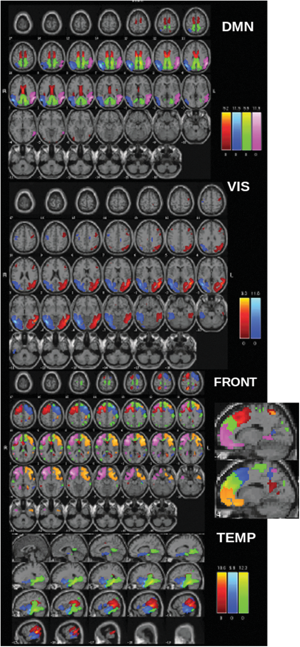
ICA component maps from resting MEG data separated into anatomic domains. Note that each color within each network represents a different IC. Please note that the same color in a different network does not necessarily represent the same region. DMN: pink and blue, inferior parietal/angular gyrus; green, cingulate (isthmus); red, posterior cingulate; FRONT, primarily frontal components (some overlap with cingulate areas); TEMP, primarily temporal components. DMN, default mode network; IC, independent component; ICA, independent component analysis; MEG, magnetoencephalography; VIS, visual components.

Furthermore, unlike with fMRI, these data should contain a minimum of artifact components (in the present case we found no artifact components) due to noise reduction and artifact removal during preprocessing. As with fMRI, subject-specific maps and timecourses were estimated using a back-reconstruction approach based on PCA compression and projection (Calhoun et al., 2001; Erhardt et al., 2011b; Houck et al., 2017). Although a beamformer source space analysis technique has been used in a similar manner before (as input to an ICA) (Houck et al., 2017), we show here that the MNE/dSPM measure used in this way gives reasonable and arguably more focal (although not point-like) components. This may be due to the differential sensitivity of MNE-based methods to connectivity in non-event related potential (ERP) data (Hincapié et al., 2017).

Furthermore, simulation has shown that MNE provides better connectivity estimation than beamformers if the interacting sources are simulated as extended cortical patches with high within-source coherence (Hincapié et al., 2017). Which method to use is also an important consideration when correlations between sources may lead to partial or full signal cancellation in the beamformer. Finally, a k-means clustering, dFNC, and meta-state analysis were conducted between all 32 components (Table 1), following the same procedure described above for fMRI.

One question that needed to be addressed was the length of the window to use for the dFNC analysis. For fMRI we chose to follow a well-established precedent of a 22-TR window ( = 44 sec) (Allen et al., 2014). Such a long time window was not considered for the MEG data since we were interested in investigating the faster oscillations available from this modality. We therefore chose a 4-sec window length for the analysis. This allowed us to capture our range of frequencies of interest (1–25 Hz), giving us the ability to see connections at higher frequencies unavailable via the fMRI analysis while avoiding “washing out” information from higher frequencies with too long a window (see the Window Size and MEG Data section in Supplementary Data for how window size effects results).

In addition, the decision of how many cluster states to use in the MEG dFNC analysis presented some questions. First was whether the MEG dFNC should closely parallel the fMRI dFNC steps. This was abandoned for two reasons: (1) due to the temporal resolution of the MEG data, there was no a priori reason to expect that the two modalities would reveal the same number of states and (2) different quantities of data were evaluated, with 60 sec of 50 Hz data in the MEG case (i.e., 3000 sampling points), as opposed to 300 sec with a 2-sec TR in the fMRI (i.e., 150 sampling points).

We initially used the Gap and Silhouette methods to estimate the number of k-means cluster states, however, we found that due to a single outlier individual the cluster state suggestion was unstable. Investigation of two, three, four, and five cluster states indicated that four state was optimal for the present data set, as this gave stable, replicable results that consistently grouped all the data from the single outlier individual into its own cluster state, and also gave reasonable occupancy percentages for the remaining three states (i.e., the percentage of correlation maps in each meaningful state was 19%, 64%, and 17%). The state that contained the outlier did not return any statistics for the group analysis since it did not contain sufficient data (i.e., only a single individual entered that state and all data for that individual were associated with that state), this state was removed from all additional analyses and did not influence any of the results shown.

Finally, we summarized the temporal behavior of the resulting cluster states, which are now allowed to overlap in time, into meta-states; that is, a representation of how much a given subject is in each of the cluster states at each point in time. Global statistics was then calculated on the meta-states and compared between HC and SP groups. Recall these are: “number of states,” “change between states,” “state span,” and “total distance.”

Results

dFNC and meta-state statistics of fMRI data

We found that 4 k-means cluster states characterized the temporal dynamics of a 5-min eyes-open resting-state fMRI scan, for both HC and SP, with a minimum of 24 participants entering each state at some point during the 5 min of data collection (Fig. 2A). Furthermore, we found that for some cluster states, SP and HC spent significantly different amounts of time there, as determined by dwell time. Particularly, SP visited and remained in state 1 for a significantly longer time than HC, whereas for state 3 the trend was reversed, with HC remaining in that state for a significantly longer time (Fig. 2B). On average, schizophrenia patients spent less time than HC in a state typified by strong, large-scale connectivity (state 3, many correlations showing r > 0.5). No significant interindividual variability between groups was found for any cluster state.

FIG. 2.

(A) fMRI k-means cluster states derived from ICA components, for HC and SP groups, number of participants who entered each state is indicated at the bottom of each plot. Color coded as follows: light blue, subcortical; light green, auditory; pink, sensory motor; orange, cerebellar; light purple, visual; yellow, DMN; blue, attention; dark green, frontal. Insets show view of dFNC as correlation grids (components × components) in same network order (top to bottom). (B) Average amount of time HC and SP spend in each state, that is, dwell time. (C) Global meta-state statistics for HC versus SP groups. All t-tests represent HC-SP. *Indicates significance at p < 0.05, FDR corrected. FDR, false discovery rate; fMRI, functional magnetic resonance imaging; dFNC, dynamic functional network connectivity; HC, healthy controls; SP, schizophrenia patients.

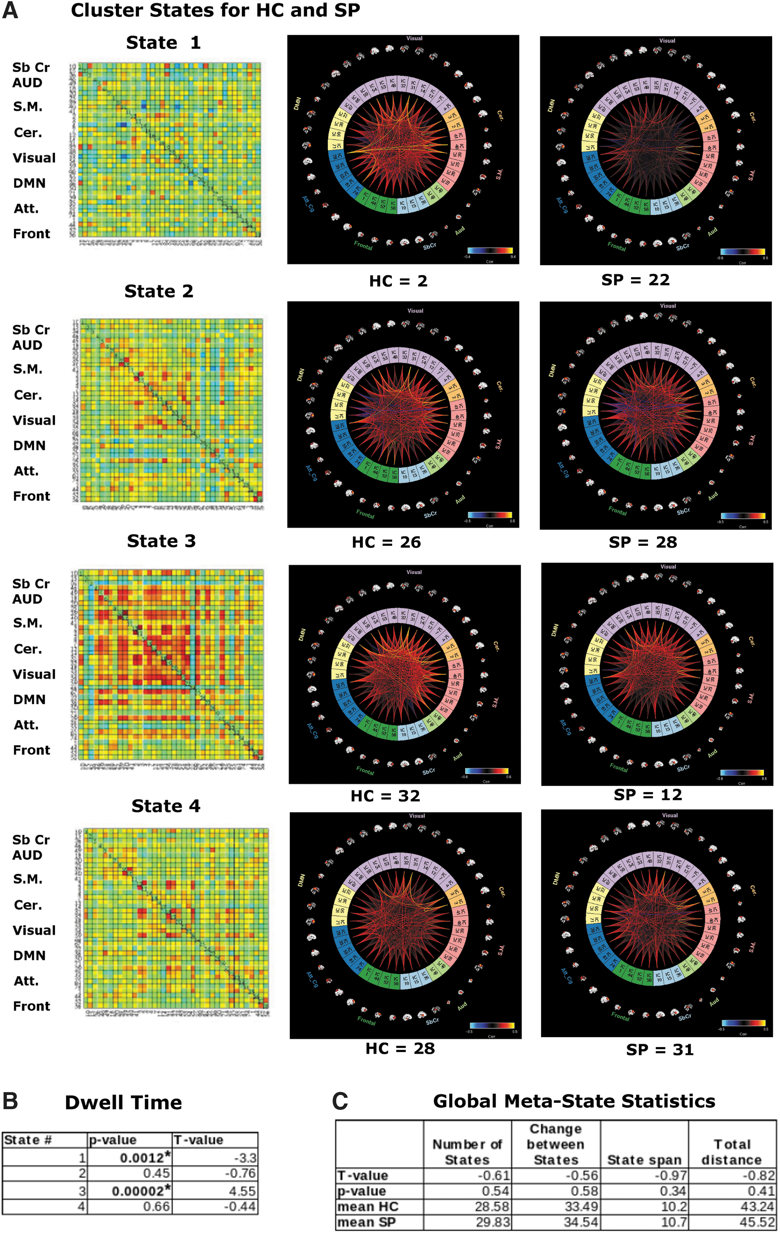
We also investigated global statistics and, for this meta-state statistics, found no significant group differences for any measures, including number of states, change between states, state span, or total distance (as defined in the Materials and Methods section; see the Distribution of Meta-state Statistics Between HC and SP Groups section in Supplementary Data for plots of the distribution of the meta-state statistics).

dFNC and meta-state statistics of MEG data

We found that 3 k-means cluster states were stable and characterized the temporal dynamics for 1 min of eyes-open resting MEG data, for both HC and SP, where a minimum of 58 participants entered each state at some point during the 1 min of data investigated (Fig. 3A). We found a significant overall between-group difference for state 2, with more variability for SP than for HC (i.e., a statistically significant difference was observed in interindividual variability for how closely each group resembled the state).

FIG. 3.

(A) MEG k-means cluster states derived from ICA components, for HC and SP groups, number of participants who entered each state is indicated at the bottom of each plot. Color coded as follows: light blue, auditory; light green, sensory motor; pink, inferior parietal; orange, visual; light purple, DMN; yellow, MTL; blue, precuneus; dark green, frontal; red, temporal pole. Insets show view of dFNC as correlation grids (components × components) in same network order (top to bottom). (B) Average amount of time HC and SP spent in each state, that is, dwell time. (C) Global meta-state statistics for HC versus SP groups. All t-tests represent HC-SP. *Indicates significance at p < 0.05, FDR corrected. MTL, medial temporal lobe.

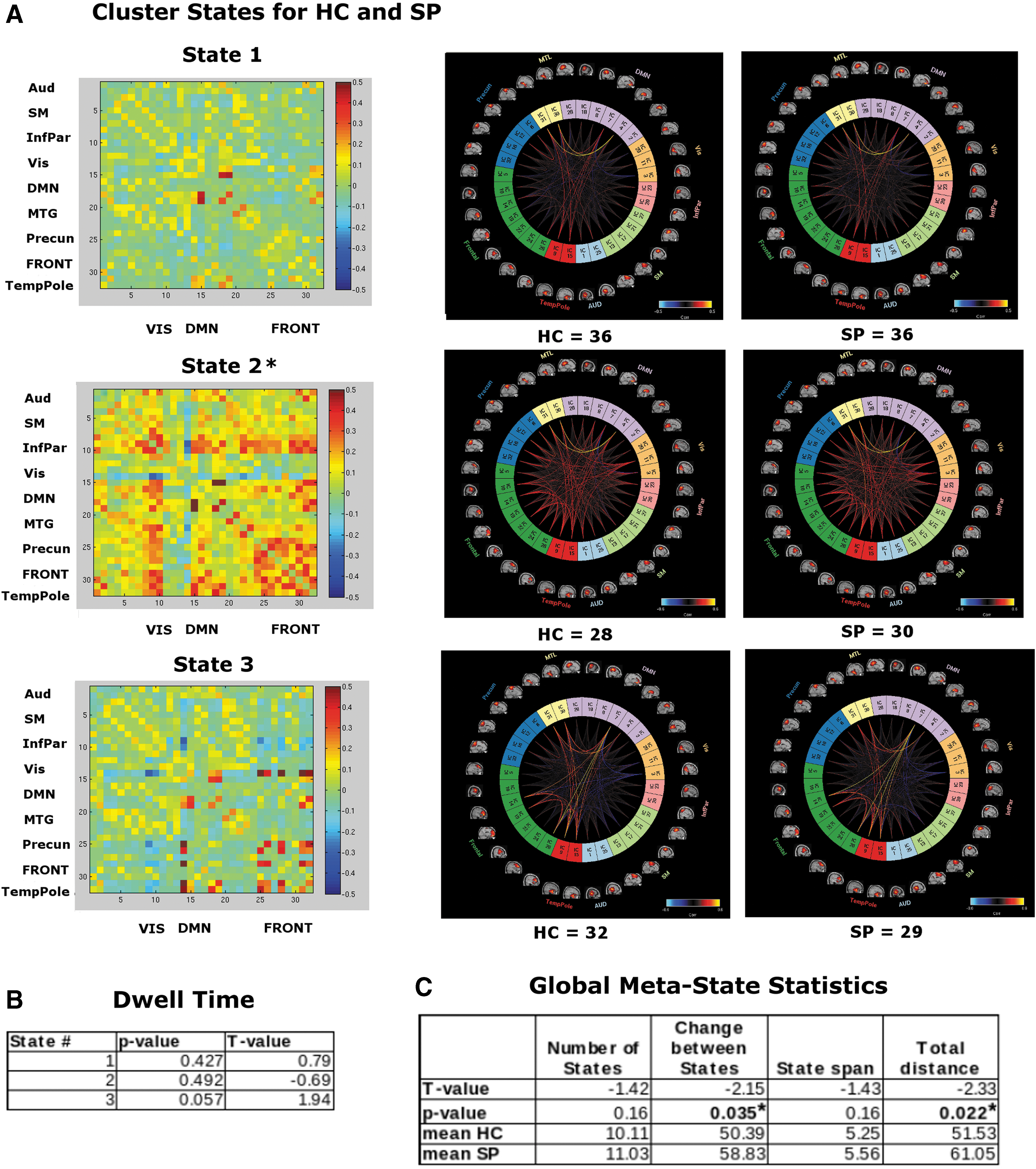
In contrast to the fMRI results, we found no group differences in dwell time between HC and SP groups (Fig. 3B). However, in these data, we see group differences in the global meta-state statistics “change between states” and “total distance” (Fig. 3C; see the Distribution of Meta-state Statistics Between HC and SP Groups section in Supplementary Data for plots of the distribution of the meta-state statistics).

Discussion

dFNC of fMRI and MEG: do they provide complementary information?

Our fMRI results, which reveal that SP spent significantly less time in a highly connected brain state (dwell time, state 3 Fig. 2B), parallel and replicate those of Damaraju et al. (2014), although we investigated an eyes-open resting state in contrast to the eyes-closed paradigm used in their study. However, for meta-state statistics calculated from fMRI data, we found no significant group differences for any measures, including number of states, change between states, state span, or total distance (as defined in the Materials and Methods section). This is in contrast to Miller et al. (2014, 2016) who introduced and investigated these statistics between HC and SP in eyes-closed resting data and found significant “reduced connectivity dynamism” in all statistics for SP relative to HC for these global statistics.

Of additional note is that the directionality (i.e., which group, HC or SP, showed the higher mean value) of all four global meta-state statistics is in the opposite direction as found in Miller et al. (2014), with HC exhibiting less movement between states than SP. However, we again point out that an eyes-open resting state was used for the present study and with a smaller sample size, whereas Miller used an eyes-closed resting state, both potentially effecting which states were detected and how frequently they are visited (McAvoy et al., 2012).

Our MEG dFNC results revealed a significant overall between-group difference for state 2, with more variability for SP than for HC (i.e., significant difference was observed in interindividual variability for how closely each group resembled the centroid of the cluster state). Because this state includes many high correlations between frontofrontal and frontoparietal regions (i.e., r > 0.5), this group difference is in keeping with numerous results that indicate that there is a frontal dysfunctional connectivity (i.e., dysconnectivity) (Bullmore et al., 1997; Friston and Frith, 1995) for SP, a dysconnectivity seen both among frontal regions, for example, insula and lateral frontal cortex (Palaniyappan et al., 2013) and between frontal regions and more distal areas, particularly frontoparietal control network regions (Roiser et al., 2013; Wu et al., 2017).

We also saw a strong correlation between activity in bilateral medial temporal gyrus and parahippocampus for all cluster states and groups, a relationship that may deserve additional investigation due to the involvement in memory, particularly recollection (Eichenbaum et al., 2007), as well as to everyday functioning in SP (Hanlon et al., 2012). It appears that the timescale of the MEG data may be attuned for such study.

In contrast to the fMRI results, we found no group differences in dwell time between HC and SP groups (Fig. 3B). However, it is in these data that we see group differences in some of the global meta-state statistics, specifically the “change between states” and the “total distance” (Fig. 3C). Recall these are the number of times that subjects switch from one meta-state to another and the overall distance traveled by each subject through the state space (the sum of the L1 distances between successive meta-states), respectively. This indicates that not only are SP changing states more often than HC but they are also changing to states that are more different in comparison with the previous state occupied.

Interestingly, and something that should be investigated further, we find that in all cases, global meta-state statistics occurs in the same direction even when failing to reach significance. In other words, SP show higher mean values for meta-state statistics relative to HC for both the MEG and fMRI analyses in the present study, reversed from what was found in Miller et al. (2014) for an eyes-closed resting state. In addition, since there is no definitive answer to the question of the optimal number of clusters (i.e., the optimal number of clusters is always somewhat subjective and depends on both the method used for measuring similarities and the parameters used for partitioning), we returned to the analysis and determined that for a choice of two cluster states, results are consistent with what has been reported; for example, fMRI showed differences between HC and SP in dwell time, but no significant meta-state statistic differences.

In the present study, we found that the information gained from a dFNC analysis of resting-state data of the same participants differs between the neuroimaging modalities of fMRI (differences seen in cluster state-level statistics) and MEG (differences seen mostly in global-level meta-state statistics). Therefore, the fusion of these modalities is expected to reveal additional information (Calhoun and Liu, 2016), potentially informing identification/classification (e.g., individuals may have comorbidities), new treatment targets, and/or potential treatment success. The next step includes determining the best way of combining these data within an overarching framework to maximize the information from each modality and the combination (e.g., joint-ICA).

The major limitations of the present study were the use of only 1 min of MEG data for the analyses and the downsampling of the MEG data to 20 ms necessitated by computing time and memory constraints, which resulted in an upper frequency limit of 25 Hz, and therefore, an inability to probe gamma-band relationships at this time. We are currently working on implementing a faster method for the analysis and will soon have hardware supplying additional memory resources alleviating these shortcomings. Arguably, one could travel to a greater number of distinct “states” were one to have more time to do so, although of course both HC and SP had the same limitation. In addition, were this the case, we would argue that many more than three viable states would have been detected in the 1-min MEG data analyzed.

A higher sampling rate could plausibly reveal more interactions and transitions (including gamma-band), however, a preliminary analysis with a 10 ms sampling rate (50 Hz maximum frequency) revealed similar results to those presented here. It has been conjectured that even 5 min of data (an often used scan duration for fMRI) may be too short for dFNC determined from fMRI data. Indeed, improvements in the reliability of resting-state data tend to rise with scan length, plateauing at a scan length of 13 min (Birn et al., 2013). Consistent with this finding, Liuzzi et al. (2017) showed that large improvements in repeatability were apparent when using a 10-min, compared with a 5-min, recording for MEG resting-state functional connectivity analyses. However, that study was looking for a single “canonical” state, whereas the present study, using windowed correlations and k-means clustering, is evaluating a set of states whose number is data driven, which may have a different, perhaps shorter, optimal scan duration.

It has been shown that FNC states in electrophysiological data can be quite transient (100–200 ms), suggesting that the resting brain is changing between different patterns of repeated activity at a rapid pace at the neuronal temporal scale (Vidaurre et al., 2016). Clearly, the timescales of these states need further investigation. However, regardless of the time scale, imaging modality, or underlying biological signal, the primary finding across studies, including the present study, is that d/FNC evolves as a multistable process passing through multiple and reoccurring discrete brain states, rather than varying in a more continuous sense (Allen et al., 2014; Cabral, et al., 2016; Hansen et al., 2015; Hutchison et al., 2013; Preti et al., 2017).

Conclusions

Our results here show how two neuroimaging modalities, MEG and fMRI, can each reveal distinct differences between HC and SP groups, and how the differences emerge in different metrics for each modality. For the eyes-open resting state investigated, we found group differences at the “cluster level” for fMRI (i.e., dwell time), whereas for MEG, we found differences at what has been referred to as the “global level” (i.e., change between states and distance traveled) (Miller et al., 2014). This indicates the importance of future work that usefully combines these two neuroimaging methodologies, taking advantage of the distinct information contained in each, to, for example, better differentiate clinical populations with overlapping symptoms, for example, using a joint ICA.

However, it is notable that some cluster states have similar structures, which could potentially influence the meta-state-level statistics. Future work will also aim to identify which metrics correlate with illness characteristics such as symptoms, chronicity, and cognitive impairment. In addition, we presented a novel MEG analysis pipeline, which incorporates a source space analysis (MNE/dSPM) as input to a group ICA, the networks/components of which may then be used for a dFNC analysis.

Footnotes

Acknowledgments

Research reported in this publication was supported by the National Institute on General Medical Sciences, National Institute on Alcohol Abuse and Alcoholism, and National Institute of Biomedical Imaging and Bioengineering of the National Institutes of Health under award numbers P20GM103472, K01AA021431, R01EB006841, and R01REB020407. Additional support was provided by NSF grant 1539067. The content is solely the responsibility of the authors and does not necessarily represent the official views of the National Institutes of Health or the National Science Foundation.

Author Disclosure Statement

No competing financial interests exist.

References

Abrol

, Chaze

, Damaraju

, Calhoun

. 2016. The chronnectome: evaluating replicability of dynamic connectivity patterns in 7500 resting fMRI datasets. Conf Proc IEEE Eng Med Biol Soc, 2016:5571–5574.

Ahonen

, Hamalainen

, Ilmoniemi

, Kajola

, Knuutila

, Simola

, Vilkman

. 1993. Sampling theory for neuromagnetic detector arrays. IEEE Trans Biomed Eng, 40:859–869.

Aine

, Bockholt

, Bustillo

, Canive

, Caprihan

, Gasparovic

, et al. 2017. Multimodal neuroimaging in schizophrenia: description and dissemination. Neuroinformatics, 15:343–364.

Alamian

, Hincapie

, Combrisson

, Thiery

, Martel

, Althukov

, Jerbi

. 2017. Alterations of intrinsic brain connectivity patterns in depression and bipolar disorders: a critical assessment of magnetoencephalography-based evidence. Front Psychiatry, 8:41.

Allen

, Damaraju

, Eichele

, Wu

, Calhoun

. 2018. EEG signatures of dynamic functional network connectivity states. Brain Topogr, 31:101–116.

Allen

, Damaraju

, Plis

, Erhardt

, Eichele

, Calhoun

. 2014. Tracking whole-brain connectivity dynamics in the resting state. Cereb Cortex, 24:663–676.

Allen

, Erhardt

, Damaraju

, Gruner

, Segall

, Silva

, et al. 2011. A baseline for the multivariate comparison of resting-state networks. Front Syst Neurosci, 5:2.

Baker

, Brookes

, Rezek

, Smith

, Behrens

, Probert Smith

, Woolrich

. 2014. Fast transient networks in spontaneous human brain activity, eLife, 3:e01867.

Besl

, McKay

. 1992. A method for registration of 3-D shapes. In IEEE Transactions on Pattern Analysis and Machine Intelligence—Special Issue on Interpretation of 3-D Scenes—Part II Archive, vol. 14, IEEE Computer Soceity, pp. 239–256.

10.

Birn

, Molloy

, Patriat

, Parker

, Meier

, Kirk

, et al. 2013. The effect of scan length on the reliability of resting-state fMRI connectivity estimates. Neuroimage, 83:550–558.

11.

Biswal

, Yetkin

, Haughton

, Hyde

. 1995. Functional connectivity in the motor cortex of resting human brain using echo-planar MRI. Magn Reson Med, 34:537–541.

12.

Biswal

BB.

2012. Resting state fMRI: a personal history. Neuroimage, 62:938–944.

13.

Bridwell

, Wu

, Eichele

, Calhoun

. 2013. The spatiospectral characterization of brain networks: fusing concurrent EEG spectra and fMRI maps. Neuroimage, 69:101–111.

14.

Brookes

, Hale

, Zumer

, Stevenson

, Francis

, Barnes

, et al. 2011a. Measuring functional connectivity using MEG: methodology and comparison with fcMRI. Neuroimage, 56:1082–1104.

15.

Brookes

, Woolrich

, Luckhoo

, Price

, Hale

, Stephenson

, et al. 2011b. Investigating the electrophysiological basis of resting state networks using magnetoencephalography. Proc Natl Acad Sci U S A, 108:16783–16788.

16.

Bullmore

, Frangou

, Murray

, 1997. The dysplastic net hypothesis: an integration of developmental and dysconnectivity theories of schizophrenia. Schizophr Res, 28:143–156.

17.

Buzsáki

, Draguhn

. 2004. Neuronal oscillations in cortical networks. Science, 304:1926–1929.

18.

Cabral

, Kambeitz-Ilankovic

, Kambeitz

, Calhoun

, Dwyer

, von Saldern

, et al. 2016. Classifying schizophrenia using multimodal multivariate pattern recognition analysis: evaluating the impact of individual clinical profiles on the neurodiagnostic performance. Schizophr Bull, 42(Suppl 1):S110–S117.

19.

Calhoun

, Adali

, Pearlson

, Pekar

. 2001. A method for making group inferences from functional MRI data using independent component analysis. Hum Brain Mapp, 14:140–151.

20.

Calhoun

, Miller

, Pearlson

, Adali

. 2014. The chronnectome: time-varying connectivity networks as the next frontier in fMRI data discovery. Neuron, 84:262–274.

21.

Calhoun

, Sui

. 2016. Multimodal fusion of brain imaging data: a key to finding the missing link(s) in complex mental illness. Biol Psychiatry Cogn Neurosci Neuroimaging, 1:230–244.

22.

Cetin

, Houck

, Rashid

, Agacoglu

, Stephen

, Sui

, et al. 2016. Multimodal classification of schizophrenia patients with MEG and fMRI data using static and dynamic connectivity measures. Front Neurosci, 10:466.

23.

Conner

, Ellmore

, Pieters

, DiSano

, Tandon

. 2011. Variability of the relationship between electrophysiology and BOLD-fMRI across cortical regions in humans. J Neurosci, 31:12855–12865.

24.

Dale

, Fischl

, Sereno

. 1999. Cortical surface-based analysis. I. Segmentation and surface reconstruction. Neuroimage, 9:179–194.

25.

Dale

, Liu

, Fischl

, Buckner

, Belliveau

, Lewine

, Halgren

. 2000. Dynamic statistical parametric mapping: combining fMRI and MEG for high-resolution imaging of cortical activity. Neuron, 26:55–67.

26.

Damaraju

, Allen

, Belger

, Ford

, McEwen

, Mathalon

, et al. 2014. Dynamic functional connectivity analysis reveals transient states of dysconnectivity in schizophrenia. Neuroimage Clin, 5:298–308.

27.

Dong

, Wang

, Chang

, Luo

, Yao

. 2018. Dysfunction of large-scale brain networks in schizophrenia: a meta-analysis of resting-state functional connectivity. Schizophr Bull, 44:168–181.

28.

, Pearlson

, Yu

, He

, Lin

, Sui

, et al. 2016. Interaction among subsystems within default mode network diminished in schizophrenia patients: a dynamic connectivity approach. Schizophr Res, 170:55–65.

29.

Eichenbaum

, Yonelinas

, Ranganath

. 2007. The medial temporal lobe and recognition memory. Annu Rev Neurosci, 30:123–152.

30.

Engel

, Singer

. 2001. Temporal binding and the neural correlates of sensory awareness. Trends Cogn Sci, 5:16–25.

31.

Erhardt

, Allen

, Damaraju

, Calhoun

. 2011a. On network derivation, classification, and visualization: a response to Habeck and Moeller. Brain Connect, 1:105–110.

32.

Erhardt

, Rachakonda

, Bedrick

, Allen

, Adali

, Calhoun

. 2011b. Comparison of multi-subject ICA methods for analysis of fMRI data. Hum Brain Mapp, 32:2075–2095.

33.

First

, Gibbon

, Spitzer

, Williams

JBW

, Benjamin

. 1997. Structured Clinical Interview for DSM-IV Axis II Personality Disorders (SCID-II). Washington, DC: American Psychiatric Press, Inc.

34.

Fischl

, Sereno

, Dale

. 1999. Cortical surface-based analysis. II: inflation, flattening, and a surface-based coordinate system. Neuroimage, 9:195–207.

35.

Fox

, Abram

, Reilly

, Eack

, Goldman

, Csernansky

, et al. 2017. Default mode functional connectivity is associated with social functioning in schizophrenia. J Abnorm Psychol, 126:392–405.

36.

Friston

, Frith

, 1995. Schizophrenia: a disconnection syndrome?. Clin Neurosci, 3:89–97.

37.

Gardner

, Murphy

, O'Donnell

, Centorrino

, Baldessarini

. 2010. International consensus study of antipsychotic dosing. Am J Psychiatry, 167:686–693.

38.

Gramfort

, Luessi

, Larson

, Engemann

, Strohmeier

, Brodbeck

, et al. 2014. MNE software for processing MEG and EEG data. Neuroimage, 86:446–460.

39.

Hall

, Robson

, Morris

, Brookes

. 2014. The relationship between MEG and fMRI. Neuroimage, 102(Pt 1):80–91.

40.

Hamalainen

, Hari

, Ilmoniemi

, Knuutila

, Lounasmaa

. 1993. Magnetoencephalography-theory, instrumentation, and applications to noninvasive studies of the working human rain. Rev Mod Phys, 65:413–497.

41.

Hamalainen

, Sarvas

. 1989. Realistic conductivity geometry model of the human head for interpretation of neuromagnetic data. IEEE Trans Biomed Eng, 36:165–171.

42.

Hanlon

, Houck

, Klimaj

, Caprihan

, Mayer

, Weisend

, et al. 2012. Frontotemporal anatomical connectivity and working-relational memory performance predict everyday functioning in schizophrenia. Psychophysiology, 49:1340–1352.

43.

Hansen

, Battaglia

, Spiegler

, Deco

, Jirsa

. 2015. Functional connectivity dynamics: modeling the switching behavior of the resting state. Neuroimage, 105:525–535.

44.

Harvey

, Vansteensel

, Ferrier

, Petridou

, Zuiderbaan

, Aarnoutse

, et al. 2013. Frequency specific spatial interactions in human electrocorticography: V1 alpha oscillations reflect surround suppression. Neuroimage, 65:424–432.

45.

Himberg

, Hyvarinen

, Esposito

. 2004. Validating the independent components of neuroimaging time series via clustering and visualization. Neuroimage, 22:1214–1222.

46.

Hincapié

A-S

, Kujala

, Mattout

, Pascarella

, Daligault

, Delpuech

, et al. 2017. The impact of MEG source reconstruction method on source-space connectivity estimation: a comparison between minimum-norm solution and beamforming. Neuroimage, 156:29–42.

47.

Houck

, Cetin

, Mayer

, Bustillo

, Stephen

, Aine

, et al. 2017. Magnetoencephalographic and functional MRI connectomics in schizophrenia via intra- and inter-network connectivity. Neuroimage, 145(Pt A):96–106.

48.

Hutchison

, Womelsdorf

, Allen

, Bandettini

, Calhoun

, Corbetta

, et al. 2013. Dynamic functional connectivity: promise, issues, and interpretations. Neuroimage, 80:360–378.

49.

Jafri

, Pearlson

, Stevens

, Calhoun

. 2008. A method for functional network connectivity among spatially independent resting-state components in schizophrenia. Neuroimage, 39:1666–1681.

50.

Khanna

, Pascual-Leone

, Michel

, Farzan

. 2015. Microstates in resting-state EEG: current status and future directions. Neurosci Biobehav Rev, 49:105–113.

51.

Kunii

, Kamada

, Ota

, Kawai

, Saito

. 2013. Characteristic profiles of high gamma activity and blood oxygenation level-dependent responses in various language areas. Neuroimage, 65:242–249.

52.

Lachaux

, Fonlupt

, Kahane

, Minotti

, Hoffmann

, Bertrand

, Baciu

. 2007. Relationship between task-related gamma oscillations and BOLD signal: new insights from combined fMRI and intracranial EEG. Hum Brain Mapp, 28:1368–1375.

53.

Leonardi

, Van De Ville

. 2015. On spurious and real fluctuations of dynamic functional connectivity during rest. NeuroImage, 104:430–436.

54.

Liao

, Cao

, Xia

, He

. 2017. Individual differences and time-varying features of modular brain architecture. Neuroimage, 152:94–107.

55.

Liuzzi

, Gascoyne

, Tewarie

, Barratt

, Boto

, Brookes

. 2017. Optimising experimental design for MEG resting state functional connectivity measurement. Neuroimage, 155:565–576.

56.

Lloyd

SP.

1982. Least squares quantization in PCM. IEEE Trans Inform Theory, 28:129–137.

57.

Madden

, Parks

, Tallman

, Boylan

, Hoagey

, Cocjin

, et al. 2017. Sources of disconnection in neurocognitive aging: cerebral white-matter integrity, resting-state functional connectivity, and white-matter hyperintensity volume. Neurobiol Aging, 54:199–213.

58.

McAvoy

, Larson-Prior

, Ludwikow

, Zhang

, Snyder

AZ.

, Gusnard

DL.

2012. Dissociated mean and functional connectivity BOLD signals in visual cortex during eyes closed and fixation. J Neurophysiol, 108:2363–2372.

59.

Meier

, Tewarie

, Hillebrand

, Douw

, van Dijk

, Stufflebeam

, Van Mieghem

. 2016. A mapping between structural and functional brain networks. Brain Connect, 6:298–311.

60.

Miller

, Yaesoubi

, Calhoun

. 2014. Higher dimensional analysis shows reduced dynamism of time-varying network connectivity in schizophrenia patients. Conf Proc IEEE Eng Med Biol Soc, 2014:3837–3840.

61.

Miller

, Yaesoubi

, Turner

, Mathalon

, Preda

, Pearlson

, et al. 2016. Higher dimensional meta-state analysis reveals reduced resting fMRI connectivity dynamism in schizophrenia patients. PLoS One, 2016; 11:e0149849.

62.

Mosher

, Leahy

, Lewis

. 1999. EEG and MEG: forward solutions for inverse methods. IEEE Trans Biomed Eng, 46:245–259.

63.

Muthukumaraswamy

, Singh

. 2008. Spatiotemporal frequency tuning of BOLD and gamma band MEG responses compared in primary visual cortex. Neuroimage, 40:1552–1560.

64.

Nashiro

, Sakaki

, Braskie

, Mather

. 2017. Resting-state networks associated with cognitive processing show more age-related decline than those associated with emotional processing. Neurobiol Aging, 54:152–162.

65.

Niessing

, Ebisch

, Schmidt

, Niessing

, Singer

, Galuske

. 2005. Hemodynamic signals correlate tightly with synchronized gamma oscillations. Science, 309:948–951.

66.

Nishida

, Morishima

, Yoshimura

, Isotani

, Irisawa

, Jann

, et al. 2013. EEG microstates associated with salience and frontoparietal networks in frontotemporal dementia, schizophrenia and Alzheimer's disease. Clin Neurophysiol, 124:1106–1114.

67.

Nugent

, Luber

, Carver

, Robinson

, Coppola

, Zarate

Jr . 2017. Deriving frequency-dependent spatial patterns in MEG-derived resting state sensorimotor network: a novel multiband ICA technique. Hum Brain Mapp, 38:779–791.

68.

Palaniyappan

, Simmonite

, White

, Liddle

. 2013. Neural primacy of the salience processing system in schizophrenia. Neuron, 79:814–828.

69.

Preti

, Bolton

, Van De Ville

. 2017. The dynamic functional connectome: state-of-the-art and perspectives. Neuroimage, 160:41–54.

70.

Rieger

, Diaz Hernandez

, Baenninger

, Koenig

. 2016. 15 Years of microstate research in schizophrenia—where are we?. A meta-analysis. Front Psychiatry, 7:22.

71.

Roiser

, Wigton

, Kilner

, Mendez

, Hon

, Friston

, Joyce

. 2013. Dysconnectivity in the frontoparietal attention network in schizophrenia. Front Psychiatry, 4:176.

72.

Roopun

, Cunningham

, Racca

, Alter

, Traub

, Whittington

. 2008. Region-specific changes in gamma and beta2 rhythms in NMDA receptor dysfunction models of schizophrenia. Schizophr Bull, 34:962–973.

73.

Sakoğlu

, Pearlson

, Kiehl

, Wang

, Michael

, Calhoun

. 2010. A method for evaluating dynamic functional network connectivity and task-modulation: application to schizophrenia. MAGMA, 23:351–366.

74.

Scheeringa

, Fries

, Petersson

, Oostenveld

, Grothe

, Norris

, et al. 2011. Neuronal dynamics underlying high- and low-frequency EEG oscillations contribute independently to the human BOLD signal. Neuron, 69:572–583.

75.

Scott

, Courtney

, Wood

, de la Garza

, Lane

, King

, et al. 2011. COINS: an innovative informatics and neuroimaging tool suite built for large heterogeneous datasets. Front Neuroinform, 5:33.

76.

Taulu

, Kajola

, Simola

. 2004. Suppression of interference and artifacts by the Signal Space Separation Method. Brain Topogr, 16:269–275.

77.

Taulu

, Simola

. 2006. Spatiotemporal signal space separation method for rejecting nearby interference in MEG measurements. Phys Med Biol, 51:1759–1768.

78.

Uusitalo

, Ilmoniemi

. 1997. Signal-space projection method for separating MEG or EEG into components. Med Biol Eng Comput, 35:135–140.

79.

Van de Ville

, Britz

, Michel

. 2010. EEG microstate sequences in healthy humans at rest reveal scale-free dynamics. Proc Natl Acad Sci U S A, 107:18179–18184.

80.

Vergara

, Miller

, Calhoun

. 2017. An information theory framework for dynamic functional domain connectivity. J Neurosci Methods, 284:103–111.

81.

Vidaurre

, Quinn

, Baker

, Dupret

, Tejero-Cantero

, Woolrich

. 2016. Spectrally resolved fast transient brain states in electrophysiological data. Neuroimage, 126:81–95.

82.

Wang

, Saalmann

, Pinsk

, Arcaro

, Kastner

. 2012. Electrophysiological low-frequency coherence and cross-frequency coupling contribute to BOLD connectivity. Neuron, 76:1010–1020.

83.

Werner

, Malaspina

, Rabinowitz

. 2007. Socioeconomic status at birth is associated with risk of schizophrenia: population-based multilevel study. Schizophr Bull, 33:1373–1378.

84.

, Zeng

, Shen

, Yuan

, Qin

, Zhang

, Hu

. 2017. Functional network connectivity alterations in schizophrenia and depression. Psychiatry Res, 263:113–120.

85.

Zaehle

, Frund

, Schadow

, Tharig

, Schoenfeld

, Herrmann

. 2009. Inter- and intra-individual covariations of hemodynamic and oscillatory gamma responses in the human cortex. Front Hum Neurosci, 3:8.

86.

Zhu

, Zumer

, Lowenthal

, Padberg

, Recanzone

, Krubitzer

, et al. 2009. The relationship between magnetic and electrophysiological responses to complex tactile stimuli. BMC Neurosci, 10:4.

Supplementary Material

Please find the following supplemental material available below.

For Open Access articles published under a Creative Commons License, all supplemental material carries the same license as the article it is associated with.

For non-Open Access articles published, all supplemental material carries a non-exclusive license, and permission requests for re-use of supplemental material or any part of supplemental material shall be sent directly to the copyright owner as specified in the copyright notice associated with the article.

0.00 MB

0.56 MB