Characteristic Fluctuations Around Stable Attractor Dynamics Extracted from Highly Nonstationary Electroencephalographic Recordings

Experimental design

In total, we consider 72 recordings of 41 subjects, which are divided into 20 recordings of 9 epilepsy patients, 10 sleep recordings of 10 healthy subjects, and 42 recordings of 21 healthy subjects in resting state during eyes-open and eyes-closed conditions. Data have been recorded in four different laboratories, using different EEG equipment and data preprocessing routines.

Sleep data

Sleep of 10 right-handed neurologically healthy subjects recorded in the Sleep Laboratory of the Faculty of Psychology of the National Autonomous University of Mexico participated in this study, after giving written informed consent. Table 1 provides information about the participants and the percentage of time they stayed in each sleep stage.

Before the study, all subjects had a structured clinical interview and kept a 15-day sleep log. Only those with regular sleeping habits and no symptoms of sleep disorders, history of medical, psychiatric or neurological disorders, drug or medication were included. The protocol was approved by the Ethical Committee of the Faculty of Medicine of the National Autonomous University of Mexico and followed the ethical standards of the Declaration of Helsinki (1964).

All subjects slept two nights at the laboratory, the first for adaptation to recording procedures and the second for EEG analysis. Standard polysomnography (PSG) and a standard scalp EEG were recorded at Fp1, Fp2, F3, F4, F7, F8, C3, C4, T3, T4, T5, T6, P3, P4, O1, O2, Fz, Cz, and Pz of the 10–20 International System (Lesser, 1986) referenced to A1 with a Grass 8–20 polygraph with filters set at 0.1 and 70 Hz for EEG, at 10 and 70 for EMG, and 0.3 and 70 Hz for EOG. All night PSG data were digitized and stored with 1024 Hz sampling rate and using a 12-bit A–D converter of the GRASS-GAMMA acquisition program.

Wakefulness and sleep stages were identified by standard procedures using 30-sec epochs (Rechtschaffen and Kales, 1968). Percentages were calculated over the total recording time of the whole night. Sleep stage percentages as shown in Table 1 correspond in general terms with the values expected for young adults (Williams et al., 1974).

Epilepsy patients

EEG data were recorded from nine patients (five men and four women; age range 21–45 years) suffering from pharmacoresistant temporal lobe epilepsy. Subjects have been under presurgical evaluation at the department of neurology of the Inselspital of the University of Bern. The ethics committee of the Kanton of Bern approved this retrospective study. Further, all patients gave written informed consent that their EEG data might be used for research and teaching purposes.

For the EEG recordings standard 10–20 montage positions (Lesser, 1986) were used. After passing an anti-aliasing filter with a cutoff frequency of 70 Hz and an attenuation of 24 dB/oct, the EEG signals were sampled at 200 Hz (seizure 1–12) and 256 Hz (seizure 13–20) using the earlobe reference. A/D conversion had a resolution of 16 bit. EEG seizure onset and seizure offset were visually determined by an experienced electroencephalographer (K.S.) in bipolar montage. Table 2 provides information about patients and seizure durations.

Further information about the EEG recordings from epilepsy patients can be found in Müller et al. (2014).

Healthy subjects in resting state during eyes-open and eyes-closed conditions

The EEG recordings during resting state were provided from two different laboratories and contain in total 21 subjects (Table 3). In all cases, subjects were in resting state for 2 min with closed eyes and open eyes, respectively. When eyes open, they were instructed to look at a mark in the center of a computer screen. All the subjects gave written informed consent.

Eleven elderly healthy subjects (five men and six women; age range 67–94 years) have been measured in the Laboratory of the Clinical Neurophysiology of the Institute National of Medical Science and Nutrition Salvador Zubirán INCMNSZ by using the 10–20 International System (Lesser, 1986) standard scalp EEG at Fp1, Fp2, F3, F4, F7, F8, C3, C4, T3, T4, T5, T6, P3, P4, O1, O2, Fz, Cz, and Pz referenced to earlobe with filter set at 0.1–70 Hz, and the signal were sampled at 200 Hz.

The other 20 EEGs data in resting state (closed eyes and open eyes) of healthy subjects (seven women and three men; age range 23–38 years) were recorded in the Laboratory of Psychophysiology of Cognitive and Emotional Processes of the Institute of Neuroscience of the University of Guadalajara, Mexico by using an Electro-Cap with the same 19 electrodes positions of the 10–20 International System as mentioned earlier. The signals were referenced to earlobe with filter set at 0.1–70 Hz and sampled at 200 Hz and using neuronic acquisition program.

EEG data of all recordings (sleep data, resting state, and recordings from epilepsy patients) were transformed to median reference (Müller et al., 2011, 2014). All EEG signals were filtered to obtain a broadband ranging between 0.5 and 25 Hz to diminish the influence of muscle artifacts by using a fourth-order Butterworth filter. Fp1, Fp2, O1, and O2 were excluded from the analysis because usually these electrodes are mostly contaminated by blink and eye movements and muscular artifacts, respectively.

Statistical analysis

Nowadays there exists a broad palette of different interrelation measures to construct the functional brain network (Boccaletti et al., 2006), usually divided into linear and nonlinear estimators (Galka, 2000; Kantz and Schreiber, 2004; Pereda et al., 2005). Owing to the fact that single neurons, the elementary building blocks of the brain, show pronounced nonlinear dynamical properties (Keener and Sneyd, 1998) one might expect that nonlinear estimators are better suited for the extraction of relevant features from empirical time series. However, for interrelation properties it was proven that even for the favorable situation of low-dimensional stationary nonlinear systems, the performance of linear cross-correlations is highly competitive with several commonly used nonlinear measures stemming from different areas such as information theory, phase space reconstruction, or synchronization measures (Kreuz et al., 2007; Mormann et al., 2005). Also in Ansari-Asl et al. (2006) it was shown that numerically robust but simple linear measures may perform better than sophisticated algorithms, which aim to extract linear as well as nonlinear interrelations.

Based on these findings, we mainly focus in this study on the estimation of zero-lag cross-correlations. Maximum lag correlations are computed additionally to provide evidence that the observed effects are not trivial artifacts of volume conduction.

In all practical circumstances, cross-correlations are estimated over finite data segments, whose length is adjusted to balance between stationarity requirements and statistical accuracy. For a multivariate data set of M EEG channels, the zero-lag cross-correlation matrix is estimated by \documentclass{aastex}\usepackage{amsbsy}\usepackage{amsfonts}\usepackage{amssymb}\usepackage{bm}\usepackage{mathrsfs}\usepackage{pifont}\usepackage{stmaryrd}\usepackage{textcomp}\usepackage{portland, xspace}\usepackage{amsmath, amsxtra}\usepackage{upgreek}\pagestyle{empty}\DeclareMathSizes{10}{9}{7}{6}\begin{document} \begin{align*}{ C_ { ij } } = \frac { 1 } { T } \mathop \sum \limits_ { k = 1 } ^T { X_i } \left( { { t_k } } \right) { X_j } \left( { { t_k } } \right) . \tag { 1 } \end{align*} \end{document}

Here T denotes the number of samples of the data segment and \documentclass{aastex}\usepackage{amsbsy}\usepackage{amsfonts}\usepackage{amssymb}\usepackage{bm}\usepackage{mathrsfs}\usepackage{pifont}\usepackage{stmaryrd}\usepackage{textcomp}\usepackage{portland, xspace}\usepackage{amsmath, amsxtra}\usepackage{upgreek}\pagestyle{empty}\DeclareMathSizes{10}{9}{7}{6}\begin{document}$$i , j = 1 , \ldots , M$$ \end{document} are electrode numbers. In Equation (1), the data is normalized to zero mean and unit variance, such that the correlation coefficient takes values between +1 and −1. All diagonal elements are equal to one because each signal is perfectly correlated with itself. Furthermore, the matrix is real symmetric and, being a quadratic form, positive semidefinite. By using a running window approach, the correlation matrix may be estimated in a time-dependent manner.

Equation (1) can be understood as an average over the product of real values. If the two sets \documentclass{aastex}\usepackage{amsbsy}\usepackage{amsfonts}\usepackage{amssymb}\usepackage{bm}\usepackage{mathrsfs}\usepackage{pifont}\usepackage{stmaryrd}\usepackage{textcomp}\usepackage{portland, xspace}\usepackage{amsmath, amsxtra}\usepackage{upgreek}\pagestyle{empty}\DeclareMathSizes{10}{9}{7}{6}\begin{document}$${X_i} \left( k \right) , {X_j} \left( k \right)$$ \end{document} are independent random variables, the correlation coefficient is precisely zero in theory. However, as the sum in Equation (1) is taken over a finite range, numerical estimates are distributed symmetrically around zero (Müller et al., 2011). Furthermore, the shorter the data segments, the larger the probability that nonzero estimates take values notably different from zero.

In fact the situation is even worse. The magnitude of nonzero estimates depends not only on the length of the data window but also on the spectral content of the data, which may change drastically during the time course of an EEG recording (Müller et al., 2011). The larger the contribution of slow frequency components of a signal, the larger is the amount of random correlations (Rummel et al., 2010). This phenomenon, caused by the fact that cross-correlations are estimated over finite data segments (and in many practical applications over quite short segments to improve time resolution), is called “random correlation” (Laloux et al., 1999; Plerou et al., 1999).

Marín-García et al. (2013) proposed a method, which aims to obtain reliable estimates for genuine correlations with a well-defined significance level, based on the use of appropriate surrogate data. It turned out that the so-called significant average correlation (SAC) matrix performs best in terms accuracy of the results, the sensitivity to detect correlations, and the robustness against noise, in comparison with several other proposals. The matrix elements of the SAC matrix are defined as \documentclass{aastex}\usepackage{amsbsy}\usepackage{amsfonts}\usepackage{amssymb}\usepackage{bm}\usepackage{mathrsfs}\usepackage{pifont}\usepackage{stmaryrd}\usepackage{textcomp}\usepackage{portland, xspace}\usepackage{amsmath, amsxtra}\usepackage{upgreek}\pagestyle{empty}\DeclareMathSizes{10}{9}{7}{6}\begin{document} \begin{align*} SA { C_ { ij } } \left( t \right) = { \frac { { S_ { ij } } } { { N_T } } } \mathop \sum \limits_ { k = 1 } ^ { { N_T } } C_ { ij } ^k \left( t \right) . \tag { 2 } \end{align*} \end{document}

The sum is just the average over matrix elements of the cross-correlation matrix estimated over N_T data windows, numbered by the index k, each of length T, whereas \documentclass{aastex}\usepackage{amsbsy}\usepackage{amsfonts}\usepackage{amssymb}\usepackage{bm}\usepackage{mathrsfs}\usepackage{pifont}\usepackage{stmaryrd}\usepackage{textcomp}\usepackage{portland, xspace}\usepackage{amsmath, amsxtra}\usepackage{upgreek}\pagestyle{empty}\DeclareMathSizes{10}{9}{7}{6}\begin{document}$${S_{ij}}$$ \end{document} represents the result of a nonparametric significance test. To this end, a set of Shift-Surrogates (Netoff and Schiff, 2002) is created from the original data segment. Then each segment is divided into N_T data windows, and, as in the case of the original data, for each window the zero-lag cross-correlation matrix is estimated. Thereafter, we applied for each matrix element separately the Mann–Whitney–Wilcoxon (MWW) rank test to estimate the probability that correlation coefficients derived from the original data and the surrogates belong to distributions with the same median values. Including a Bonferroni correction for multiple testing at a 1% significance level, \documentclass{aastex}\usepackage{amsbsy}\usepackage{amsfonts}\usepackage{amssymb}\usepackage{bm}\usepackage{mathrsfs}\usepackage{pifont}\usepackage{stmaryrd}\usepackage{textcomp}\usepackage{portland, xspace}\usepackage{amsmath, amsxtra}\usepackage{upgreek}\pagestyle{empty}\DeclareMathSizes{10}{9}{7}{6}\begin{document}$${S_{ij}}$$ \end{document} was set to one if \documentclass{aastex}\usepackage{amsbsy}\usepackage{amsfonts}\usepackage{amssymb}\usepackage{bm}\usepackage{mathrsfs}\usepackage{pifont}\usepackage{stmaryrd}\usepackage{textcomp}\usepackage{portland, xspace}\usepackage{amsmath, amsxtra}\usepackage{upgreek}\pagestyle{empty}\DeclareMathSizes{10}{9}{7}{6}\begin{document}$$p < { \frac { 0.01 \times 2 } { \left[ { M \left( { M - 1 } \right) } \right] } } .$$ \end{document} Otherwise, \documentclass{aastex}\usepackage{amsbsy}\usepackage{amsfonts}\usepackage{amssymb}\usepackage{bm}\usepackage{mathrsfs}\usepackage{pifont}\usepackage{stmaryrd}\usepackage{textcomp}\usepackage{portland, xspace}\usepackage{amsmath, amsxtra}\usepackage{upgreek}\pagestyle{empty}\DeclareMathSizes{10}{9}{7}{6}\begin{document}$$SA{C_{ij}} \left( t \right)$$ \end{document} was set to zero.

To probe the hypothesis, of the existence of a pronounced correlation pattern that is stable in time as in Müller et al. (2014) and universal in the sense of a high similarity across subjects, we studied similarity between average genuine correlation matrices. In the case of the sleep data, we used 30 sec segments that coincided with the so-called sleep epochs used by experienced electroencephalographers (M.C.-C. and I.Y.R.-P.) for sleep scoring. These were divided into \documentclass{aastex}\usepackage{amsbsy}\usepackage{amsfonts}\usepackage{amssymb}\usepackage{bm}\usepackage{mathrsfs}\usepackage{pifont}\usepackage{stmaryrd}\usepackage{textcomp}\usepackage{portland, xspace}\usepackage{amsmath, amsxtra}\usepackage{upgreek}\pagestyle{empty}\DeclareMathSizes{10}{9}{7}{6}\begin{document}$$T = 3 \,{ \rm{sec}}$$ \end{document} nonoverlaping data windows to evaluate Equation (2). We estimated the average matrices separately for each sleep stage. In case of recordings from epilepsy patients and resting state EEG during eyes-open and eyes-closed conditions, we used segments of length 10 sec, which are divided into \documentclass{aastex}\usepackage{amsbsy}\usepackage{amsfonts}\usepackage{amssymb}\usepackage{bm}\usepackage{mathrsfs}\usepackage{pifont}\usepackage{stmaryrd}\usepackage{textcomp}\usepackage{portland, xspace}\usepackage{amsmath, amsxtra}\usepackage{upgreek}\pagestyle{empty}\DeclareMathSizes{10}{9}{7}{6}\begin{document}$${N_T} = 10$$ \end{document} nonoverlapping data windows of length \documentclass{aastex}\usepackage{amsbsy}\usepackage{amsfonts}\usepackage{amssymb}\usepackage{bm}\usepackage{mathrsfs}\usepackage{pifont}\usepackage{stmaryrd}\usepackage{textcomp}\usepackage{portland, xspace}\usepackage{amsmath, amsxtra}\usepackage{upgreek}\pagestyle{empty}\DeclareMathSizes{10}{9}{7}{6}\begin{document}$$T = 1 \;{ \rm{sec}}$$ \end{document} . Owing to the filtering, the short windows contained three and a half cycles of the slowest retained waves in all cases.

Note that the large length of a segment is due to the fact that in this contribution exclusively broadband signals are considered. For the analysis of, for example, alpha-activity much shorter segments of about 1–2 sec are already appropriate.

To quantify the statistical similarity of two average correlation matrices \documentclass{aastex}\usepackage{amsbsy}\usepackage{amsfonts}\usepackage{amssymb}\usepackage{bm}\usepackage{mathrsfs}\usepackage{pifont}\usepackage{stmaryrd}\usepackage{textcomp}\usepackage{portland, xspace}\usepackage{amsmath, amsxtra}\usepackage{upgreek}\pagestyle{empty}\DeclareMathSizes{10}{9}{7}{6}\begin{document}$$\left\langle {SA{C_n}} \right\rangle$$ \end{document} and \documentclass{aastex}\usepackage{amsbsy}\usepackage{amsfonts}\usepackage{amssymb}\usepackage{bm}\usepackage{mathrsfs}\usepackage{pifont}\usepackage{stmaryrd}\usepackage{textcomp}\usepackage{portland, xspace}\usepackage{amsmath, amsxtra}\usepackage{upgreek}\pagestyle{empty}\DeclareMathSizes{10}{9}{7}{6}\begin{document}$$\left\langle {SA{C_m}} \right\rangle$$ \end{document} , obtained for two different segments “n” and “m,” we first ordered their nondiagonal elements in one-dimensional vectors V_n and V_m by the “vech” operation. These objects are called matrix vectors in the sequel. After normalizing these vectors to zero mean and unit variance, we estimated the pairwise correlation between them through Equation (1). Furthermore, we applied the nonparametric MWW rank test, which estimates the probability that the median off-diagonal matrix element of the two SAC matrices are different. This test has the advantage that no assumption about the underlying probability distributions of the samples is done, but the discriminative power is in general reduced when compared with parametric test statistics. Thus, estimated p values in this article can be considered as an upper limits.

Note that the Pearson coefficient estimated for different SAC matrices quantify structural similarity between these matrices, but due to normalization it is insensitive for differences in the magnitude by which a certain correlation pattern is expressed. To test statistical equivalence also for the overall strength of the stationary pattern, we applied additionally the MWW rank test.

If no significant differences between averaged SAC matrices estimated separately for different physiological stages can be found, we concluded that the average over the whole recordings is justified. The result of this overall average is termed “stationary pattern” in the sequel and will be denoted by \documentclass{aastex}\usepackage{amsbsy}\usepackage{amsfonts}\usepackage{amssymb}\usepackage{bm}\usepackage{mathrsfs}\usepackage{pifont}\usepackage{stmaryrd}\usepackage{textcomp}\usepackage{portland, xspace}\usepackage{amsmath, amsxtra}\usepackage{upgreek}\pagestyle{empty}\DeclareMathSizes{10}{9}{7}{6}\begin{document}$$\left\langle {SAC} \right\rangle$$ \end{document} . The stationary pattern of the peri-ictal recordings of epilepsy patients has already been evaluated in a similar manner (Müller et al., 2014).

To probe stability in time and further to test the hypothesis that dynamical features are imprinted in deviations from \documentclass{aastex}\usepackage{amsbsy}\usepackage{amsfonts}\usepackage{amssymb}\usepackage{bm}\usepackage{mathrsfs}\usepackage{pifont}\usepackage{stmaryrd}\usepackage{textcomp}\usepackage{portland, xspace}\usepackage{amsmath, amsxtra}\usepackage{upgreek}\pagestyle{empty}\DeclareMathSizes{10}{9}{7}{6}\begin{document}$$\left\langle {SAC} \right\rangle$$ \end{document} , we focus in the second part of this work on the time evolution of genuine cross-correlations, and likewise differences to the stationary correlation structure, by employing a running window approach.

We estimated the SAC matrix using a running window approach along the whole recordings, with a step width of 30 sec for sleep data and 10 sec epilepsy data and recordings of eyes-open and eyes-closed conditions during rest. For each window, we then computed the correlation between the SAC matrix and the stationary pattern \documentclass{aastex}\usepackage{amsbsy}\usepackage{amsfonts}\usepackage{amssymb}\usepackage{bm}\usepackage{mathrsfs}\usepackage{pifont}\usepackage{stmaryrd}\usepackage{textcomp}\usepackage{portland, xspace}\usepackage{amsmath, amsxtra}\usepackage{upgreek}\pagestyle{empty}\DeclareMathSizes{10}{9}{7}{6}\begin{document}$$\left\langle {SAC} \right\rangle$$ \end{document} . To summarize the results concerning the temporal stability of the stationary pattern of all subjects, we provided medians and the 95% confidence interval of the Pearson correlations estimated separately for each sleep stage, eyes-open and eyes-closed conditions, or, respectively, separately for the preictal, ictal, and postictal intervals. Small confidence intervals are then indicators for a high temporal stability of \documentclass{aastex}\usepackage{amsbsy}\usepackage{amsfonts}\usepackage{amssymb}\usepackage{bm}\usepackage{mathrsfs}\usepackage{pifont}\usepackage{stmaryrd}\usepackage{textcomp}\usepackage{portland, xspace}\usepackage{amsmath, amsxtra}\usepackage{upgreek}\pagestyle{empty}\DeclareMathSizes{10}{9}{7}{6}\begin{document}$$\left\langle {SAC} \right\rangle$$ \end{document} across all subjects.

Finally, to probe our second hypothesis, we determined in which manner deviations from the stationary pattern were capable to distinguish different physiological states and compared the results with a classical strategy, namely cross-correlation values itself. For this purpose, we calculated the average of the absolute value of the nondiagonal elements of the SAC matrices \documentclass{aastex}\usepackage{amsbsy}\usepackage{amsfonts}\usepackage{amssymb}\usepackage{bm}\usepackage{mathrsfs}\usepackage{pifont}\usepackage{stmaryrd}\usepackage{textcomp}\usepackage{portland, xspace}\usepackage{amsmath, amsxtra}\usepackage{upgreek}\pagestyle{empty}\DeclareMathSizes{10}{9}{7}{6}\begin{document} \begin{align*} \left\langle { \left\vert { SA { C^l } } \right\vert } \right\rangle = \frac { 2 } { { M \left( { M - 1 } \right) } } \mathop \sum \limits_ { i > j } ^M \left\vert { SAC_ { ij } ^l } \right\vert , \tag { 3 } \end{align*} \end{document}

obtained for a particular sleep stage, for the eyes-open and eyes-closed conditions, or, respectively, the different phases of the peri-ictal transition, across all subjects. Thereafter, we computed from this set of real numbers the median and the 95% confidence interval separately for each physiological state.

Finally, we also considered deviations from the average matrix (Equation 2): \documentclass{aastex}\usepackage{amsbsy}\usepackage{amsfonts}\usepackage{amssymb}\usepackage{bm}\usepackage{mathrsfs}\usepackage{pifont}\usepackage{stmaryrd}\usepackage{textcomp}\usepackage{portland, xspace}\usepackage{amsmath, amsxtra}\usepackage{upgreek}\pagestyle{empty}\DeclareMathSizes{10}{9}{7}{6}\begin{document} \begin{align*}{D_{ij}} \left( t \right) = SA{C_{ij}} \left( t \right) - \left\langle {SA{C_{ij}}} \right\rangle \tag{4} \end{align*} \end{document}

Note that to evaluate characteristic deviations of a particular physiological stage, this difference matrix can be used in Equation (3) instead of \documentclass{aastex}\usepackage{amsbsy}\usepackage{amsfonts}\usepackage{amssymb}\usepackage{bm}\usepackage{mathrsfs}\usepackage{pifont}\usepackage{stmaryrd}\usepackage{textcomp}\usepackage{portland, xspace}\usepackage{amsmath, amsxtra}\usepackage{upgreek}\pagestyle{empty}\DeclareMathSizes{10}{9}{7}{6}\begin{document}$$SA{C_{ij}}$$ \end{document} .

Model calculations

To substantiate the interpretation of the observed phenomena, which we provide in the Discussion section, we performed additionally some model calculations of explicit nonstationary dynamical systems. In a first step, we estimated the correlation matrix of two strongly coupled Rössler systems, where each of the variables of the six-dimensional phase space were erratically perturbed by independent Gaussian white noise. Because the random perturbations have been frequently applied (every 250 time steps), the system is almost permanently located on a transient around the attractor and is thus nonstationary by definition. Then we estimated the average of the six-dimensional correlation matrix and compared the outcome with the equivalent nonperturbed system.

In the second case, we deformed the attractor (actually we considered a mixed system) showing that in this case the correlation matrix strongly depended on such deformations. Here time series are derived as a mixture of the strongly coupled Rössler system and a system of two anticorrelated Lorenz oscillators. The mixture has been varied gradually along the time course such that at the first time step the recording consisted of the pure Rössler systems and at the last time step the anticorrelated Lorenz systems remain. In this way, we permanently deform the invariant set of the whole system.

A detailed description of the differential equations, chosen parameters as well as the numerical results can be found in the Supplementary Data (Supplementary Data are available online at www.liebertpub.com/brain).

Existence of a pronounced stationary correlation pattern

In a first step, we searched for stationary correlation pattern. Based on the findings published in Müller et al. (2014), such pattern is supposed to be independent of the physiological state, namely, a particular sleep stage. In Figure 1, we show mean correlation matrices from the recording of subject 9, where averages have been taken over all 30 sec segments of the whole night, but separately for each sleep stage. A similar figure of a young and an old adult with eyes open and eyes closed is presented in the Supplementary Data (Supplementary Fig. S1).

OPEN IN VIEWER

FIG. 1.

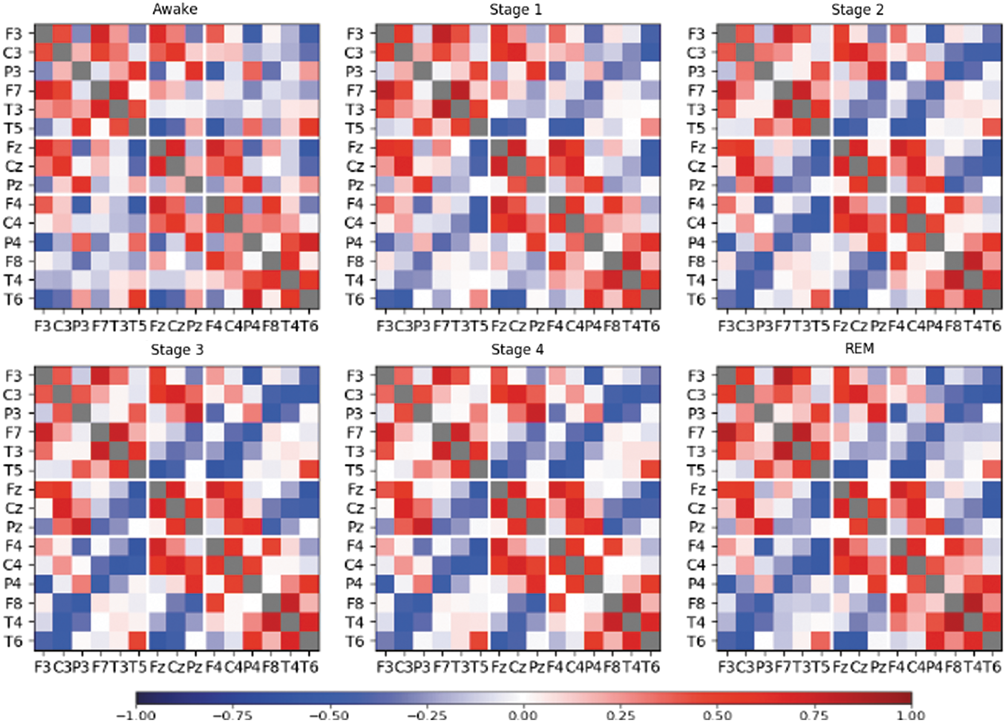
Average correlation matrices of subject 9 of Table 1. Each average is taken over all data segments belonging to a particular sleep stage. Color images available online at www.liebertpub.com/brain

In close similarity with findings derived from the scalp EEG recordings of epilepsy patients (Müller et al., 2014), we here observe a pronounced correlation structure in all sleep stages (as well as for eyes-open and eyes-closed conditions), despite the marked electrophysiological and neurophysiological differences between REM, non-REM, and the awake state. Similar to Müller et al. (2014), positive correlations are more prominent for connections within the same hemisphere, whereas diagonal contralateral electrode pairs tend to be anticorrelated. Considering furthermore the high noise level of scalp EEGs and the nonstationarity of the brain activity, the appearance of high magnitude average cross-correlations is a counterintuitive result.

The intriguing similarity of the pronounced correlation patterns shown in Figure 1 leads to the question whether an average over the whole recording without distinguishing sleep stages is justified. To substantiate such procedure, we estimated for all subjects the correlation between all pairs of the average correlation matrices obtained separately for the sleep stages. We found that average SAC matrices of different sleep stages are indeed highly correlated with Pearson coefficients >0.9. Furthermore, we compared quantitatively the equivalence of the median off-diagonal matrix elements by using the MWW rank test, without finding significant differences.

In consequence, we found that despite drastic physiological differences, marked morphological changes of the EEG recordings between sleep stages as well as alternations of the functional network, we observed a similar pronounced average correlation pattern. The same is true for the comparison of the eyes-open and eyes-closed conditions. Pearson coefficients encountered surprisingly high estimates. Consequently, we conclude according to these findings that the average over the whole recording, termed as “stationary pattern” in the sequel, is justified. Corresponding results and a detailed discussion can be found in the Supplementary Data (see Supplementary Figs. S2 and S3 in the Supplementary Data).

Stability over time and temporal fluctuations

In the following step, we study the temporal stability of the correlation coefficients to further probe for the stationarity of the average correlation pattern. For this purpose, we estimated the correlation between the stationary pattern and SAC matrices estimated with a running window approach and visualized the time course of all 105 matrix elements of the SAC matrix. Results for subject 9 are provided in Figure 2.

OPEN IN VIEWER

FIG. 2.

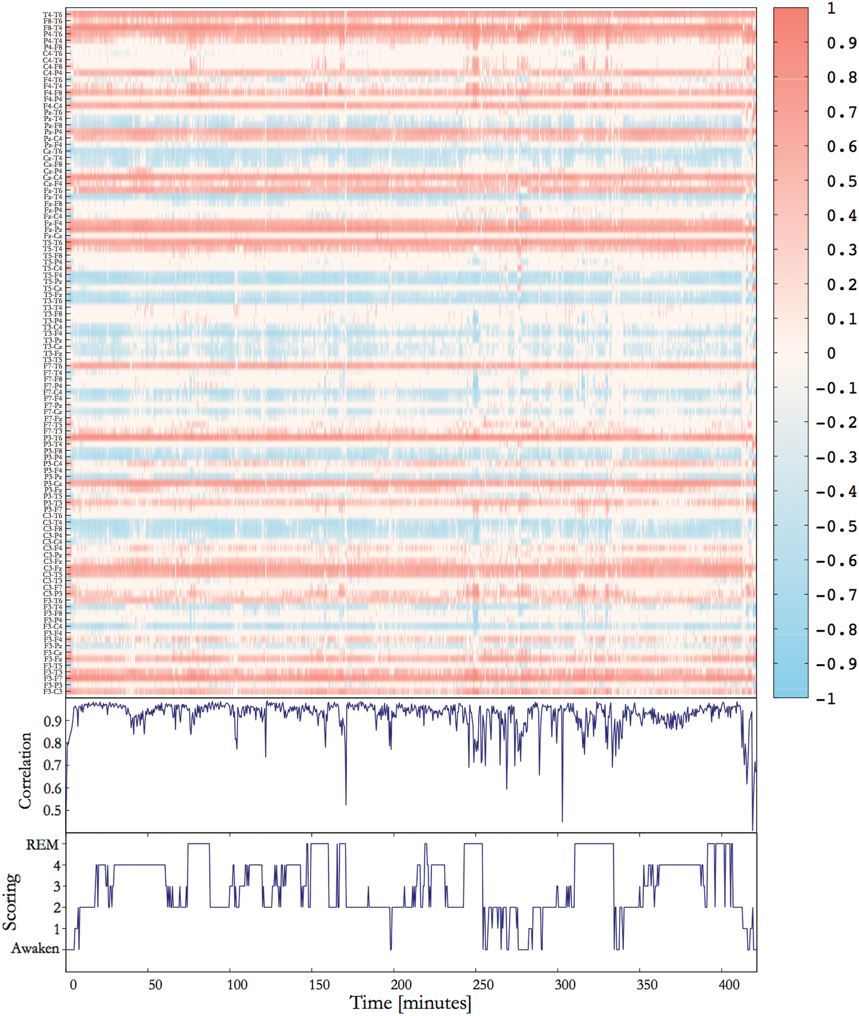
Case study of subject 9. Upper panel: Time evolution of all 105 correlation coefficients of the SAC matrix. Middle panel: Correlation between the time-dependent matrix vectors formed from the SAC matrix and the stationary pattern. Lower panel: Scoring of the corresponding polysomnography. SAC, significant average correlation. Color images available online at www.liebertpub.com/brain

In Figure 2, we observe that the correlation between the SAC matrix and the stationary pattern is almost always >0.85, which constitutes an extremely high value. Only at the beginning of the recording, one notices a gradual increase of correlations up to values of about 0.95. After this initial phase, the correlation appears to be quite stable and even outliers (e.g., during short waking stages between minute 250 and 300) never drop <0.6, which still implies a pronounced similarity. Furthermore, such minimal values are encountered only for short moments and appear as sharp spikes in Figure 2. Besides such short episodes, the correlation of the time-dependent SAC matrix with the stationary pattern is considerably high and fluctuates around 0.9.

The visual inspection of the time course of the SAC matrix elements (upper panel of Fig. 2) confirms these results. Despite pronounced changes of the spectral composition as well as significant topological alternations of the functional network during sleep cycles (Achermann and Borbély, 1998; Cantero et al., 2000; Corsi-Cabrera et al., 1987, 2003; De Gennaro et al., 2001; Duckrow and Zaveri, 2005; Gast et al., 2014; Guevara et al., 1995; Kaminski et al.,1997; Llinás and Ribary, 1993; Nielsen et al., 1990; Pérez-Garci et al., 2001; Voss et al., 2009) the majority of the matrix elements never change their sign and fluctuations around some nonzero constant value seem negligible. Matrix elements with a low average magnitude show noteworthy fluctuations, whereas the overall impression of Figure 2 resembles a remarkably stable correlation pattern. Even transitions between sleep stages are hardly visible.

Note that this observation does not imply a lack of interesting dynamical features imprinted in the EEG signals, and we do not challenge the highly nonstationary character of such recordings. On the contrary, we believe, that the extraction of such nonstationary features provides important and novel progresses for the understanding of the brain dynamics. On this ground, the observation of a stable scaffold of functional connectivity is even more surprising.

The results obtained for all subjects (Fig. 3) corroborate these observations. For all sleep stages, the medians are about 0.85 and fluctuations are remarkably small. Only for the waking state (and partly for the transitional stage 1) one observes a considerable amount of fluctuations. However, the median of the correlation coefficient during waking state is about 0.87 and the lower value of the 95% confidence interval of the cross-correlations is still >0.5. Furthermore, one observes that the fluctuations during sleep stages are not generated by a large discrepancy between subjects. Median values estimated for each subjects separately are almost always >0.9. Only a few subjects and only during sleep stages 3 and 4 encounter values between 0.85 and 0.9 and also the comparably large fluctuations during the awake state cannot be explained by variations across subjects, given that, besides the exception of two subjects, all medians are clearly >0.85. However, 90% confidence intervals are considerably larger for the wake state than for all sleep stages.

OPEN IN VIEWER

FIG. 3.

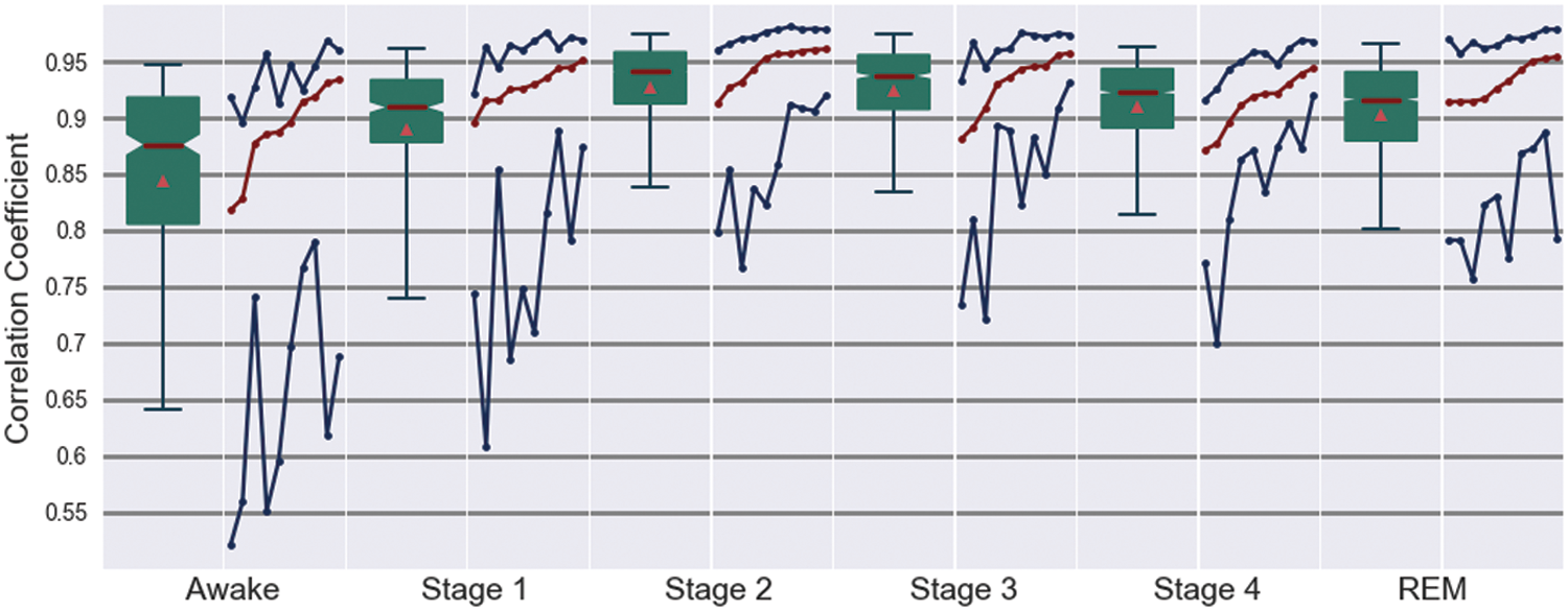
Summary statistics over all 10 subjects of Table 1. For each sleep stage two columns are drawn. The box plot on the left shows median value and the borders of the 50% and 90% confidence interval of the Pearson correlations estimated between the SAC matrix of a given data window and the stationary pattern. Furthermore, as a red triangle, the average value is shown. The right column shows median (red color) and the borders of the 90% confidence interval (blue color) separately for the 10 healthy subjects, ordered by ascending median correlation. Solid lines are just for guidance of the eye. Color images available online at www.liebertpub.com/brain

Based on these results, one may conclude that there exists a kind of rigid skeleton of oscillatory interrelations between brain regions covering the whole scalp. This spatially extended but stable structure could be advantageous for an efficient communication between different, probably distant brain sites. On the one hand, it might coordinate global dynamical features of widely interconnected neuronal populations and additionally it may admit that local deformations of this structure quickly propagate to cover larger spatial scales. Hence, such a skeleton could balance between segregation of local activity and global information integration (Singer, 1999; Tononi, 2004, 2010; Tononi and Edelman, 1998). Consequently, this picture suggests that transient dynamical features should manifest themselves through deviations from this structure. Accordingly, one should expect that the waking state, with a major variety of different kind of activity, is characterized by larger fluctuations around the stationary pattern as shown in Figure 3.

Subject-specific or generic feature

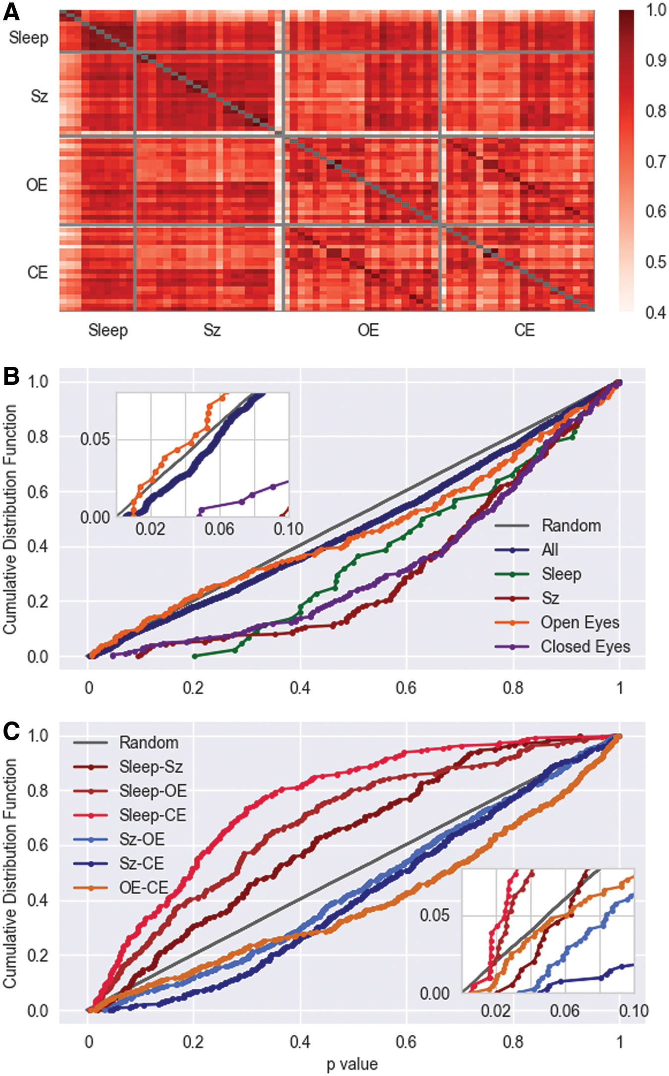
The question remains whether the pronounced stationary correlation pattern represents individual signatures of the brain dynamics of a single person, such as a stationary dynamical fingerprint of neural activity, or, whether it is a generic phenomenon, which reflects general principles of brain functioning. To answer this question, we compare in Figure 4 the stationary pattern obtained for each EEG recording, namely, sleep and resting state EEGs as well as the epilepsy recordings.

OPEN IN VIEWER

FIG. 4.

(A) Pearson coefficients for the pairwise comparison stationary pattern. Considered are sleep recordings (sleep), the peri-ictal average of focal onset SZ, resting state for EO and EC for young and elderly adults. Young adults are the first half of the resting state recordings, elderly adults the second half. (B) Cumulative distributions of p values derived by the nonparametric Mann–Whitney–Wilcoxon rank test for the pairwise comparison of the stationary pattern of all recordings (blue symbols), the 10 sleep recordings (green), the 20 peri-ictal averages of temporal lobe seizures (brown), open (orange) and closed eyes (purple). As a reference we also draw the results of 100,000 samples of Gaussian white noise with the same size as the empirical data (gray-shaded squares). The inset shows the left tail of the distributions (C) Same as (B) but now the stationary pattern of sleep EEGs is compared with the results for seizure EEGs (dark brown), open eyes (light brown), and closed eyes condition (red). Furthermore, seizure data is compared with open- (light blue) and closed-eyes (dark blue) conditions, and finally a pairwise comparison with open and closed eyes (orange) is shown. CE, closed eyes; EEG, electroencephalographic recordings; OE, open eyes; SZ, seizures. Color images available online at www.liebertpub.com/brain

In Müller et al. (2014), it was already found that mean correlation matrices, estimated over periods of several minutes, show also a marked correlation pattern, which, as in this case, seem to be independent of the physiological state of the subject. Namely, average matrices derived from the preseizure, postseizure, or the seizure period show a remarkable similarity [Pearson correlations are always higher than 0.6; Fig. 3 of Müller et al. (2014)] and also peri-ictal averages of different subjects are surprisingly similar. Pearson coefficients are >0.5 [Fig. 4 of Müller et al. (2014)]. Smallest values are obtained exclusively for the comparison with recording 20 of the epilepsy patients, which already has been identified as an outlier (Müller et al., 2014). Furthermore, by visual inspection one gains the impression that the stationary pattern obtained from this pathological activity shares many features with the structures observed for the sleep data.

The Pearson coefficient quantifies topological similarity between the average correlation pattern, which turns out to be considerably high for all cases (Fig. 4A). Only for the pairwise comparisons with the mentioned recording 20 of the epilepsy patients and one recording of the young adults during resting state (EO and EC-condition) the correlation values drop slightly >0.5, whereas, in general, Pearson coefficients are considerably >0.6. Furthermore, a certain structure of the matrix shown in Figure 4A can be identified. First one can observe that the sleep EEG segregates in two clusters (subject 1–3 and 4–10), where the stationary pattern are extremely similar within these clusters, given that the Pearson correlations take values about 0.9, whereas intercluster correlations are, in general, smaller. Furthermore, one identifies a high similarity between the second cluster and almost all remaining recordings, independently whether the pathological case of epilepsy or healthy subjects during rest are considered. The peri-ictal average of the seizure EEGs, in contrast, correlates stronger with the resting state EEGs of older subjects than those obtained for young adults, independently where eyes are open or closed during rest.

But most importantly one observes nonambiguously that also resting state EEGs fall into two similarity clusters, which separate young and old adults. Whereas almost no difference between EO and EC conditions can be noticed for both groups, Pearson coefficients between these groups are systematically lower, which may indicate that although the stationary pattern seemingly does not depend on the physiological state, it may evolve with the age of the subjects.

Although the Pearson coefficient is sensitive for the topological differences of the correlation pattern, the application of the MWW rank test probes similarity of the correlation strength. For comparison and, hence, as a kind of null hypothesis the cumulative distribution of p values for the comparison of white noise samples is drawn. Note that the cumulative distribution of the white noise data indicate the probability that p values occur solely by chance. Hence, a necessary condition for significance is that the smallest p values should lie above the gray straight line.

In Figure 4B, we compare average correlation matrices obtained for the same condition as, for example, all 45 pairwise comparisons of the sleep EEGs. As a result, within the same condition no significant differences can be found. However, when EEGs obtained for different conditions are compared, the sleep EEGs stand out (Fig. 4C). Independently whether they are compared with epileptic seizures, or with the eyes-closed and eyes-open conditions, the cumulative distributions are above the null hypothesis of white noise samples. However, for small p values all three curves drop below the white noise model such that only a few comparisons encounter sufficiently small p values (inset of Fig. 4C). Thus, although the three curves for the comparison with sleep EEGs are notable above the null hypothesis for a large range of p values, no significant differences between physiological conditions can be found. In addition, the results shown in Figure 4 involve multiple testing and require a Bonferroni correction, which lessens the critical p-value by a factor of 200 for the comparison of the sleep and epilepsy data. Thereby none of the obtained p values mark significant differences, a result which is corroborated by the estimation of Pearson coefficients (Fig. 4A). Further comparison of correlation matrices of different physiological stages are shown in Supplementary Figure S4.

In summary, one observes that the similarity between the stationary pattern of the sleep or resting state EEGs and the peri-ictal averages of epileptic seizures is high. Furthermore, one notices that the resting state EEGs fall into two correlation clusters, which do not distinguish between eyes-open and eyes-closed conditions but separate subjects with a notable age difference. Consequently, the high similarity between the average correlation matrices and the apparent statistical equivalence of the set of matrices lead us to the conclusion that the observed pattern is a generic feature and may reflect universal principles of the brain dynamics, which may evolve with the age of the subjects, although we do not provide sufficient quantitative support for this last suspect.

Discrimination between different physiological states

To test the hypothesis that nonstationary dynamical features are imprinted in the deviations from the stationary pattern, we compared the different sleep stages, resting state for open and closed eyes, as well as the preictal, ictal, and postictal phase by estimating the Pearson coefficient of pairs of the difference matrices (Equation 4), averaged separately for different physiological states for each of the subjects. These results should be compared with those obtained for the SAC matrix shown in Supplementary Figures S2 and S3 of the Supplementary Data as well as those presented in Figure 3 in Müller et al. (2014).

The Pearson coefficients for the comparison of the average difference matrix obtained for sleep and wakefulness are shown in Figure 5. In contrast to Supplementary Figures S1 and S2, the color scales of Figure 5 are much larger and thus the differences matrices are distributed over a much wider range, which implies that deviations from the stationary pattern constitute an improved discrimination of sleep stages. Results shown in Figure 5A and B fit to neurophysiological findings about sleep–wake cycles. NREM sleep stages 3 and 4, and to a lesser degree stage 2, are highly correlated, which is consistent with the fact that they belong to the same Thalamo-cortical oscillatory mode (Steriade and McCarley, 1990). Furthermore, one observes that pairs of average difference matrices may be anticorrelated, which indicates that deviations from the average correlation pattern are toward opposite directions in matrix space. For example, anticorrelations are observed for the comparison between the three NREM sleep stages and activated states W and REM as expected from the different physiology of REM, W, and NREM sleep (Steriade and McCarley, 1990). Also the mean difference matrix obtained for stage 1 is anticorrelated to those of stages 3 and 4. If dynamical aspects are imprinted in the deviations from the stationary pattern, the dynamics of anticorrelated sleep stages are qualitatively different. In contrast, REM sleep and stage 1, as well as REM sleep and W share rather similar features, which is consistent with the activated electrophysiological pattern of REM sleep, which hinders the differentiation of W and stage 1 sleep. Until the REMs and the muscle atony allows to recognize them as different brain states with its own physiological characteristics (Steriade and McCarley, 1990).

OPEN IN VIEWER

FIG. 5.

(A, B) Quantitative comparison of the stationary pattern derived for different sleep stages, (C) and (D) for the preseizure, seizure, and the postseizure period, and (E) and (F) for the open and closed eye condition of young and elderly adults. (A), (C), and (E) display the cumulative distribution of p values derived from the Mann–Whitney–Wilcoxon rank test; (B), (D), and (F) display the corresponding Pearson coefficients. Color images available online at www.liebertpub.com/brain

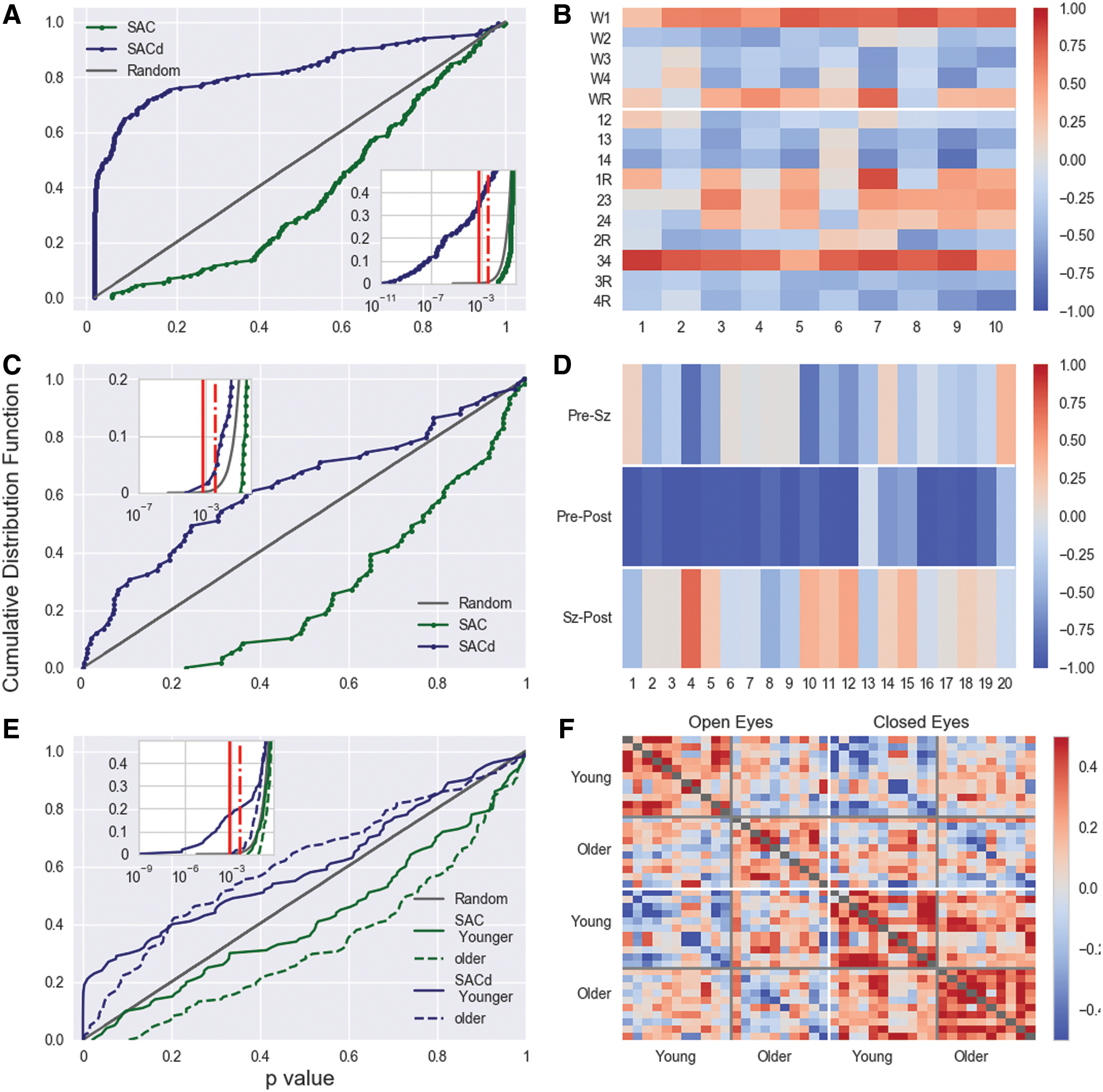
It is conspicuous that stage 2 sleep is identified as qualitatively different from stages 3 and 4 in some subjects. The same is true for the comparison between stage 1 and the awake state. However, these results are not unexpected given that sleep stages 1 and 2 are transitional stages toward stages 2 and 4 as well as REM, respectively.

The p values derived from the MWW rank test confirmed the results obtained for the Pearson coefficients (Fig. 5A). We observed a high discriminative power when deviations from the stationary pattern were considered. About 60% of the results derived for the difference matrix encounter p values <5% significance level. Even when a Bonferroni correction is employed about 40% of the results are still significant on a 5% level and about 33% when a significance level of 1% is desired (inset of Fig. 5A). At the same time, p values of the SAC matrix are all >5% and only six of them encounter values <0.1.

The significant results for the difference matrix are primarily observed for the comparison of sleep stage REM with stages 3 and 4, for the comparisons of stage 1 with sleep stages 2, 3, and 4 and also the comparisons of stages 2 and 4 provide mostly p values <0.05. In principle, striking similarities of the structure of the average difference matrices as displayed in Figure 5 lead also to notable high p values for the MWW rank test. For instance, the comparison of the wake state and stage 1, or the comparison of sleep stages 3 and 4, leads also to high p values when magnitudes of the correlations are under consideration.

In the case of the EEG recordings of the epileptic patients (Fig. 5C, D), one observes largest discrepancies for the comparison of difference matrices of the pre- and postseizure periods. All Pearson coefficients of this comparison are negative, namely, the average deviations from the stationary pattern are diametrically different, a clear indication of the effect the epileptic activity on the electrical brain dynamics even after seizure termination (Gast et al., 2014; Müller et al., 2011). For the direct comparison of the preseizure with the seizure period, no consistent result could be derived. In some cases average deviations are positive, whereas in others negative correlated, which could be due to different durations of immediate preseizure states in different recordings. For the comparison of the postseizure with the seizure period, Pearson coefficients are dominantly anticorrelated, although also in this case some estimates lead to positive values.

For the comparison of the overall correlations strengths (Fig. 5C), one observes qualitatively the same results as for the sleep recordings. Average difference matrices lead to more significant differences between phases than correlation matrices themselves. However, now the outcomes are much less significant than for the sleep data such that almost none of the comparisons (of the pre with the postseizure state) lead to sufficiently small p values.

Finally, the comparison of resting states with open and closed eyes leads to some interesting observations (Fig. 5E, F). First, average distance matrices allow the distinction between the two resting state conditions. In particular for the young adults, Pearson correlations between the eyes-open and eyes-closed conditions are dominantly negative. About 15% of the p values derived from MWW rank test are below the 5% significance level (Bonferroni corrected). For elderly adults, the difference is less obvious and p values are not significant, although also in this case the outcomes turn out to be strikingly worse when average correlation matrices are used.

However, besides the distinction of different physiological conditions, also deviations from the stationary pattern seem to be age dependent. As in the case of Figure 4, correlations between the two groups for either condition take notably lower values. If, as suspected earlier, deviations from the stationary pattern indicate nonstationary dynamical aspects, it could be that not only the stationary pattern itself but also transient electrical brain activity might evolve with the age. However, given that both groups are measured in different laboratories, these remarks are rather speculative and require confirmation through further studies.

In conclusion, when analyzing deviations from the stationary pattern one obtains a more differentiated picture for dynamical changes of different physiological states than by considering cross-correlations itself. We find remarkable quantitative differences between the results derived for the SAC matrix compared with those obtained by the difference matrix. Deviations from the stationary pattern provide a highly improved discriminative power for physiologically distinct brain stages. Thus, the results presented in this article further indicate that the deviation from the temporarily stable average correlation pattern is a more appropriate measure than correlation pattern itself.

Nonstationary dynamical aspects of brain dynamics

In Figure 2, we depict the complete time course of all 105 cross-correlation coefficients of subject 9. This figure underpins the quantitative results concerning the stability in time of the stationary pattern. Apparently, most of the correlation coefficients are extremely stable and specifically do not change their signs. Transitions between sleep stages are hardly visible and the time course of the correlation between the SAC matrix and the stationary pattern encounters almost always high values. As the average cross-correlations prove to be virtually time-independent, we in the following investigate whether nonstationary aspects of brain dynamics are imprinted in the fluctuations of the cross-correlations and, specifically, which cross-correlations reflect those aspects. To answer this question, one may investigate if there is some relation between the mean value of the correlation coefficients and the size of their fluctuations. To this end, we depict in Figure 6 separately for each sleep stage the size of its 95% confidence interval versus the mean value of each correlation coefficient.

OPEN IN VIEWER

FIG. 6.

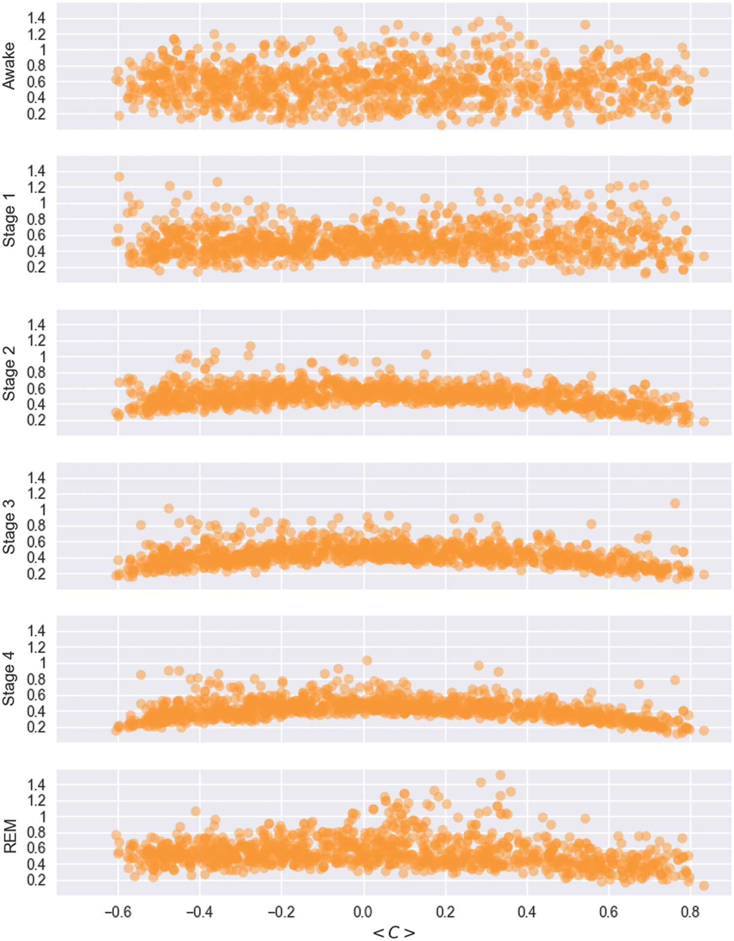
Size of the 90% confidence interval of cross-correlation coefficients in each sleep stage (ordinate) versus their mean value (abscissa) for all 10 sleep recordings. Color images available online at www.liebertpub.com/brain

One observes largest fluctuations and a tendency of lower absolute mean values during wakefulness (see also Fig. 3). The estimates of the widths of the 95% confidence intervals vary between 0.2 and 1.4 almost over the whole range of the obtained mean values. Note that correlation estimates are restricted within the range \documentclass{aastex}\usepackage{amsbsy}\usepackage{amsfonts}\usepackage{amssymb}\usepackage{bm}\usepackage{mathrsfs}\usepackage{pifont}\usepackage{stmaryrd}\usepackage{textcomp}\usepackage{portland, xspace}\usepackage{amsmath, amsxtra}\usepackage{upgreek}\pagestyle{empty}\DeclareMathSizes{10}{9}{7}{6}\begin{document}$$\left[ { - 1 , + 1} \right]$$ \end{document} such that confidence intervals are by definition smaller than 2; namely, values of the 95% confidence interval larger than 1 indicate large fluctuations around the stationary pattern. In consequence, no clear dependency between average values and fluctuation strength of the cross-correlation coefficients can be detected for the waking state. Qualitatively the same picture is obtained for sleep stage 1, although now the size of the fluctuations tends to be smaller.

This picture changes qualitatively when turning to sleep stage 2. Now one observes a clear tendency of the 95% confidence intervals: correlations coefficients with large dynamical means show smaller fluctuations and vice versa. For estimates of \documentclass{aastex}\usepackage{amsbsy}\usepackage{amsfonts}\usepackage{amssymb}\usepackage{bm}\usepackage{mathrsfs}\usepackage{pifont}\usepackage{stmaryrd}\usepackage{textcomp}\usepackage{portland, xspace}\usepackage{amsmath, amsxtra}\usepackage{upgreek}\pagestyle{empty}\DeclareMathSizes{10}{9}{7}{6}\begin{document}$$\left\langle {{C_{ij}}} \right\rangle$$ \end{document} close to zero, the fluctuations are always >0.4. In contrast, very large sizes of the 95% confidence intervals (values 1.2 or 1.4, such as observed in the case of wakefulness or sleep stage 1) are not observed. For sleep stage 2, the confidence intervals are almost always <0.7.

This behavior is even more pronounced for the distributions obtained for deep sleep, namely, sleep stages 3 and 4. Similar to sleep stage 2, the size of the average value of correlation coefficients is related to the size of its fluctuations. By trend this is also true for REM sleep.

Correlation coefficients with large average values tend to fluctuate less than those with small averages. In particular, states with higher activation levels (i.e. wakefulness, REM-sleep, and sleep stage 1), or those which are more susceptable to external stimulation (i.e. wakefulness and stage 1), or to endogenous and dream-like activity during sleep (REM sleep), show a trend toward higher fluctuations of the correlation coefficients. According to the picture depicted earlier, this result implies that those correlation coefficients with small average values are involved stronger in nonstationary dynamical aspects of the brain activity than large ones.