
Abstract
Establishing a connection between intrinsic and task-evoked brain activities is critical because it would provide a way to map task-related brain regions in patients unable to comply with such tasks. A crucial question within this realm is to what extent the execution of a cognitive task affects the intrinsic activity of brain regions not involved in the task. Computational models can be useful to answer this question because they allow us to distinguish task from nontask neural elements while giving us the effects of task execution on nontask regions of interest at the neuroimaging level. The quantification of those effects in a computational model would represent a step toward elucidating the intrinsic versus task-evoked connection. In this study we used computational modeling and graph theoretical metrics to quantify changes in intrinsic functional brain connectivity due to task execution. We used our large-scale neural modeling framework to embed a computational model of visual short-term memory into an empirically derived connectome. We simulated a neuroimaging study consisting of 10 subjects performing passive fixation (PF), passive viewing (PV), and delayed match-to-sample (DMS) tasks. We used the simulated blood oxygen level-dependent functional magnetic resonance imaging time series to calculate functional connectivity (FC) matrices and used those matrices to compute several graph theoretical measures. After determining that the simulated graph theoretical measures were largely consistent with experiments, we were able to quantify the differences between the graph metrics of the PF condition and those of the PV and DMS conditions. Thus, we show that we can use graph theoretical methods applied to simulated brain networks to aid in the quantification of changes in intrinsic brain FC during task execution. Our results represent a step toward establishing a connection between intrinsic and task-related brain activities.
Introduction
R
Neuroimaging studies have shown that performance of a cognitive task alters the intrinsic functional connectivity (FC) in nontask-related brain regions (Bluhm et al., 2011; Tommasin et al., 2017; Vatansever et al., 2015). Bluhm and colleagues, for example, found increases in FC between two “default network” brain regions (posterior cingulate/precuneus and medial prefrontal cortex [PFC]) and the rest of the brain during a visual working memory task as compared with a passive fixation (PF) task. In another study, Tommasin and colleagues found reductions in FC between brain regions within the “default mode network” (DMN) during an auditory working memory task as compared with an eyes-open RS task. Similarly, Vatansever and colleagues found reductions in FC within DMN brain regions during a motor task as compared with an RS task.
A very powerful tool that has been used to quantify changes in intrinsic FC due to task execution employs graph theoretical methods (Adams et al., 2013; Bolt et al., 2017; Cohen and D'Esposito, 2016; Fuertinger et al., 2015; Krienen et al., 2014; Moussa et al., 2011). Graph theoretical metrics have been used in the past decade to study functional and structural brain networks as they provide ways to quantify both global network organization and local network properties (Bolt et al., 2017; Rubinov and Sporns, 2010).
A recent computational study (Lee et al., 2017) demonstrated the reliability of graph theoretical metrics obtained from simulated intrinsic brain activity. Lee and colleagues modeled brain regions as Kuramoto oscillators coupled by weights extracted from a structural connectome (Hagmann et al., 2008). After finding an optimal FC matrix (one that resembled the RS empirical connectivity matrix), they set out to compute global and local network metrics and compared them to empirically obtained graph metrics during the RS. They found that simulated brain activity can be reasonably used to model graph theoretical metrics of brain organization.
However, there is a need to test the use of graph theoretical metrics on simulated intrinsic activity during task execution. We aimed to use computational modeling and graph theoretical metrics to quantify differences in intrinsic functional brain connectivity of nontask-related brain regions due to increasing task demands.
We used a large-scale computational model of visual processing that was previously verified against single-unit recordings in nonhuman primates and empirical positron emission tomography (PET), functional magnetic resonance imaging (fMRI), and magnetoencephalography (MEG) data (Banerjee et al., 2012; Corbitt et al., 2018; Horwitz et al., 2005; Liu et al., 2017; Tagamets and Horwitz, 1998; Ulloa and Horwitz, 2016). We embedded the visual processing model in a structural connectome (Hagmann et al., 2008) to examine differences in intrinsic neural activity between three conditions: PF, passive viewing (PV), and a visual delayed match-to-sample (DMS) task. Specifically, we set out to investigate whether computational modeling and graph theoretical metrics could be used to quantify and understand intrinsic neural activity changes in nontask brain regions due to increasing task demands.
Materials and Methods
In this study, we analyzed FC derived from blood oxygen level-dependent (BOLD) fMRI time series, calculated from simulated neural activity data using the framework presented in a previous article (Ulloa and Horwitz, 2016). Although in our previous article we evaluated the FC between brain regions directly involved in executing a task, in this article, we examined the intrinsic FC in the rest of the brain (brain regions not involved in task execution). To better address that question, we performed a model parameter search to find a reasonable match between empirical and model FC. Hereunder we briefly describe the components of the framework and show how it was used to generate the simulated multisubject experiment presented in this study.
The source code of our modeling work, including simulation, analysis, and visualization scripts, is freely available at (
Visual object processing model and The Virtual Brain
Visual object processing model
Our in-house visual (Tagamets and Horwitz, 1998) object processing model consists of interconnected neuronal populations representing the cortical ventral pathway that has been shown to process primarily the features of a visual object. This stream begins in striate visual cortex, extends into the inferotemporal (IT) lobe, and projects into ventrolateral PFC (Haxby et al., 1991; McIntosh et al., 1994; Ungerleider and Mishkin, 1982). The regions that comprise the visual model include those representing primary and secondary visual cortex (V1/V2), area V4, anterior IT cortex, and PFC (Fig. 1). Each of these regions contains one or more neural populations with different functional attributes (see caption of Fig. 1 for details).
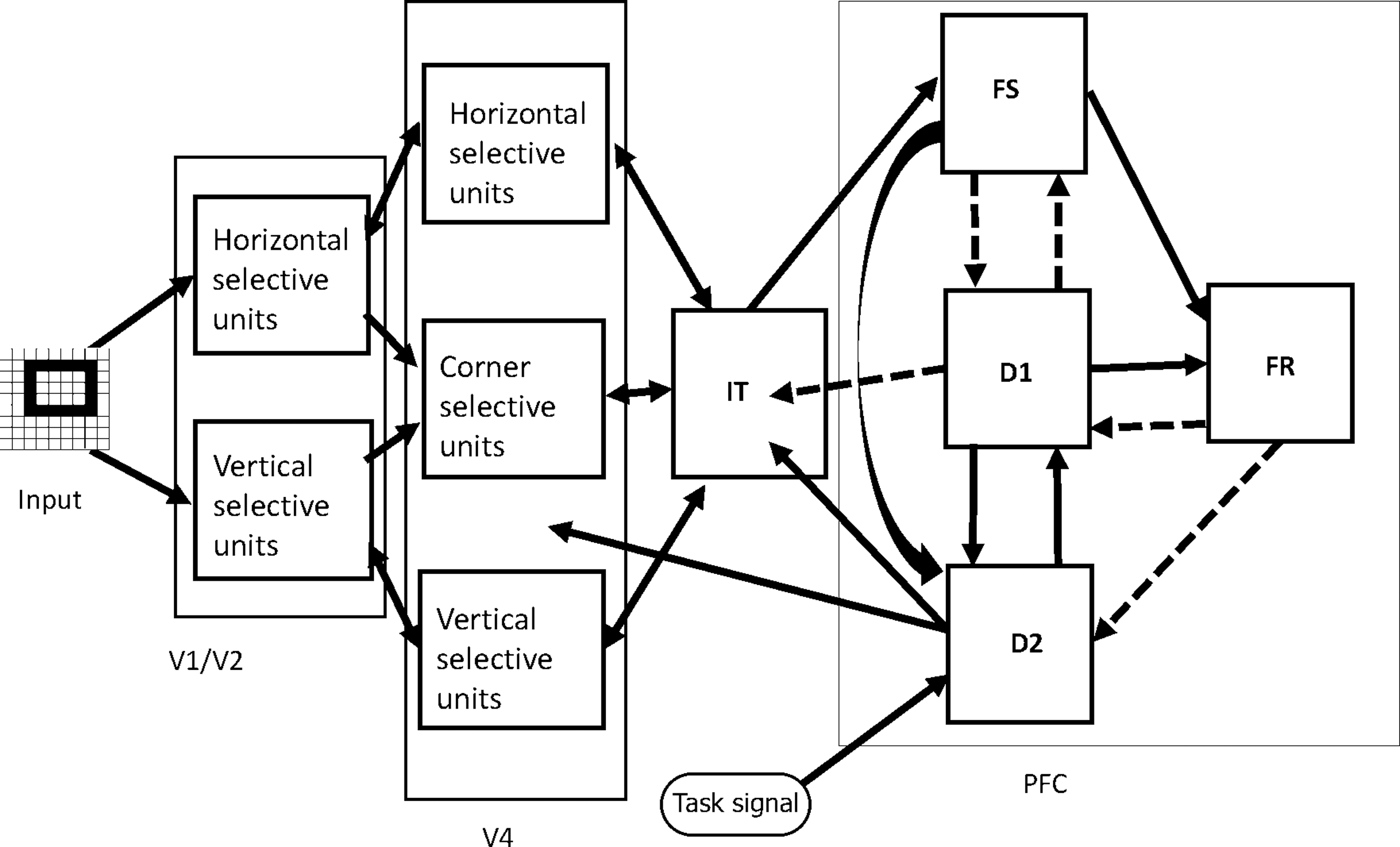
Visual short-term memory model consisted of interconnected neural populations that represent primary and secondary visual (V1/V2, V4), IT, and PFC. Each one of the submodules (shown as squares) within a given brain module is modeled with 81 (9 × 9) modified Wilson–Cowan neuronal population units. Solid arrows represent excitatory to excitatory connections and dashed arrows represent excitatory to inhibitory connections. Adapted from Horwitz and colleagues (2005). IT, inferotemporal; PFC, prefrontal cortex.
This model was designed to perform a short-term memory DMS task during each trial of which a stimulus S1 is presented for a certain amount of time, followed by a delay period in which S1 must be kept in short-term memory. When a second stimulus (S2) is presented, the model must respond as to whether S2 matches S1. The model can also perform control tasks: PF and passive perception of the stimuli (PV), in which no response is required. Multiple trials of the active and passive tasks constitute a simulated functional neuroimaging study.
The DMS-simulated experiment consisted in three trial blocks of task interspersed with rest blocks (low-attention fixation). The PV condition consists in three trial blocks of low-attention viewing of stimuli interspersed with rest blocks (low attention fixation). The PF condition consisted in low-attention fixation on a small dot throughout the simulation; there were no rest blocks in the PF condition.
The key feature used to define a visual object was shape. Model neurons in V1/V2 and V4 were assumed to be orientation selective (for simplicity, horizontal and vertical orientations were used). The structural submodels employed were based on known monkey neuroanatomical data. An important assumption for the visual model, inferred from such experimental data, was that the spatial receptive field on neurons increased along the ventral processing pathway [see Tagamets and Horwitz (1998) for details].
Each neuronal population consisted of 81 microcircuits, each representing a cortical column. The model employed modified Wilson–Cowan units (an interacting excitatory and inhibitory pair of elements for which spike rate was the measure of output neural activity) as the microcircuit (Wilson and Cowan, 1972). The input synaptic activity to each neuronal unit can also be evaluated, and combinations of this input activity were related to the fMRI BOLD signals through a forward model.
In an earlier version of the model (Horwitz et al., 2005), half the neural populations within the model were “nontask-specific” neurons that served as noise generators to “task-specific” neurons that processed shapes during the DMS task. The model generated time series of simulated electrical neuronal and synaptic activity for each module that represents a brain region. The time series of synaptic activity, convolved with a hemodynamic response function, was then used to compute simulated fMRI BOLD signal for each module representing a brain region, as well as FC among key brain regions [see Horwitz et al. (2005) for details on this method].
This model was able to perform the DMS task, generate simulated neural activities in the various brain regions that match empirical data from nonhuman preparations, and produce simulated functional neuroimaging data that generally agree with human experimental findings [see Tagamets and Horwitz (1998) and Horwitz et al. (2005) for details]. In this article, we employ the version of the model introduced by Ulloa and Horwitz (2016) in which nontask-specific neurons are replaced by noise-generated activity from neural elements in The Virtual Brain (TVB) software simulator (Sanz Leon et al., 2013).
The Virtual Brain
TVB software (Sanz Leon et al., 2013; Sanz-Leon et al., 2015) is a simulator of primarily RS brain activity that combines (1) white matter structural connections among brain regions to simulate long-range connections and (2) a given neuronal population model to simulate local brain activity. It also employs forward models that convert simulated neural activity into simulated functional neuroimaging data. TVB source code and documentation are freely available at (
In this article, for the structural model, we chose the diffusion spectrum magnetic resonance imaging-based connectome described by Hagmann and colleagues (2008), which contains 998 nodes. For the neural model for each node, we employed Wilson–Cowan population neuronal units (Wilson and Cowan, 1972) to model the local brain activity because our in-house large-scale neural model (LSNM) simulators use modified Wilson–Cowan equations as their basic neuronal unit. Our forward model that converts simulated neural activity into simulated fMRI is a modification of the Balloon-Windkessel model of Friston and colleagues (Friston et al., 2000; Stephan et al., 2007) that is included in TVB.
Integrating TVB and LSNM
To perform our computational study, we concurrently ran two neural simulators: our LSNM simulator, which generated task-driven neural activity of the brain regions directly involved in the visual DMS task, and TVB simulator (Sanz Leon et al., 2013) to generate RS neural activity in the brain regions not involved in the task. Because the task-based brain nodes were embedded within RS brain regions of interest (ROIs), we expected that the neuroimaging activity in key connectome ROIs would differ between PF, PV, and task-based simulations. In this study, we sought to quantify those differences, first by comparing the pattern of FC across conditions, then by using graph theoretical methods to quantify those differences.
Within the LSNM, connections and parameter choices closely follow those in the original articles. Likewise, the connections and parameter choices among TVB nodes closely follow those described by Sanz-Leon and colleagues (2015). There are two differences between the simulations presented in this article and the previous (Ulloa and Horwitz, 2016) article: the location of the FR units has been changed to PreSMA and the global coupling parameter has been changed (after a parameter search procedure detailed hereunder).
Task-based model node placement in TVB
The connectome derived by Hagmann and colleagues (2008) serves as a source of neural noise to our task-based neural model. Such a connectome was obtained by averaging the weighted network of five experimental subjects, where each one of the 998 nodes represents a ROI covering a surface area of ∼1.5 cm2. The connection weights among the nodes represent corticocortical connections given by white matter connection density among the given nodes. As stated previously, each node is represented by a Wilson–Cowan population unit and thus each node is assumed to comprise one excitatory and one inhibitory neural population. We implemented noise as an additive term to the stochastic Euler integration scheme provided by TVB software.
The locations of the four PFC nodes (FS, D1, D2, and FR) require some comment. The inclusion of these four neural populations in the original LSNMs was based on the electrophysiological studies of Funahashi and colleagues (1990) that found in monkey PFC four distinct neuronal responses during a delayed response task: neurons that (1) increased their activity when a stimulus was present (FS), (2) increased their activity during the delay part of the task (D1), (3) increased their activity during both when a stimulus was present and during the delay period (D2), and (4) increased their activity before making a correct response (FR). It is not known whether these neuronal types are found in separate anatomical locations in PFC or are intermixed within the same brain area, although the latter is the more likely case (except possibly for the FR population).
In the original modeling studies of Tagamets and Horwitz (1998) and Husain and colleagues (2004), the functional neuroimaging data represented a single region that included all four nodes. To illustrate the integrated synaptic activity and fMRI signal for each one of the modules of the combined LSNM/TVB model separately, we have assigned a different spatial location to each one of the four PFC submodules. We have used the Talairach coordinates of the PFC, based on Haxby and colleagues (1991), for the submodule D1 and have designated spatial locations in adjacent ROIs for the FS and D2 submodules. The FR submodule has been allocated to a spatial location determined by an fMRI study of working memory in humans (Pessoa et al., 2002). See Table 1 for coordinate locations of each module/submodule of the visual short-term memory nodes within the structural connectome.
The acronyms of the submodules in the model hereunder represent visual cortical areas (V1/V2, V4), IT cortex, and prefrontal cortex (FS: neuronal populations that respond to stimulus presentation, D1 and D2: neuronal populations that keep a memory trace of stimulus presented, and FR: neuronal population involved in short-term memory task response). Note that the locations of FS and D2 are not explicitly known (see Methods and Materials section) and were chosen only to demonstrate validity of the method.
IT, inferotemporal.
Simulating electrical activity and fMRI activity
Electrical activities of each node in Hagmann's connectome (TVB equations)
Each one of the nodes in Hagmann's connectome is represented as a Wilson–Cowan model of excitatory (E) and inhibitory (I) neuronal populations, as described in Sanz-Leon and colleagues (2015):
and
where SE
and SI
are sigmoid functions described by
where l is the number of nodes in the connectome and n is the number of LSNM units connected to a connectome node;
A global coupling parameter
Electrical activities of each LSNM unit
Each one of the submodules of the LSNM model contains 81 neuronal population units. Each one of those units is modeled as a Wilson–Cowan population of excitatory (E) and inhibitory (I) elements. The electrical activities of each one of those elements at time t are given by the following equations:
and
where
where
where
Integrated synaptic activity
Before computing fMRI BOLD activities, we compute the synaptic activity, spatially integrated over each LSNM module (or connectome node) and temporally integrated for 50 ms as described by Horwitz and Tagamets (1999)
where
Note that the first three terms mentioned are the synaptic weights from within unit i and the last term is the sum of synaptic connections originating in all other LSNM units and connectome nodes connected to unit i. Note also that in our current scheme, there are no long-range connections from inhibitory populations.
Generation of subjects and task performance of the LSNM model
We generated simulated subjects by creating several different sets of connection weights among submodules of the LSNM visual network until we obtained the number of desired subjects whose task performance was >60%. However, the weights among the nodes with TVB connectome remained unchanged across subjects. The generation of different connectome sets to simulate individual subjects is outside the scope of this article, but will be essential for future simulation studies investigating the effects of a behavioral task on nontask brain nodes.
Task performance was measured as the proportion of correct responses over an experiment. A response in the response module (FR, described in the caption of Fig. 1) was considered a correct response in each trial if at least 2 units had neuronal electrical responses more than a threshold of 0.7 during the response period. To create different sets of weights that were different from the ideal subject, we multiplied feedforward connections among modules in the LSNM visual model by a random proportion of between 0.95 and 1.
Equations for the forward fMRI BOLD model
We implemented the BOLD signal model described by Stephan and colleagues (2007). We use the output of the integrated synaptic activity mentioned as the neural state equation to the hemodynamic state equations hereunder. The BOLD signal for each ROI, y(t), is computed as follows:
where the coefficients
where V0
is the resting venous blood volume fraction, q is the deoxyhemoglobin content, v is the venous blood volume, E0
is the oxygen extraction fraction at rest,
The evolution of the venous blood volume v and deoxyhemoglobin content q is given by the balloon model hemodynamic state equations as follows:
where
where s is an exponentially decaying vasodilatory signal given by
where
RS parameter exploration
We performed a global parameter exploration (for which we used exclusively TVB simulator and the structural connectome with no task nodes) to obtain a reasonable match between empirical and model FC (Cabral et al., 2011). We obtained the empirical FC data sets from Hagmann and colleagues (2008) that we used as a target for our simulated FC. Note that we used a low resolution (66 nodes) FC of matrices to perform the comparisons between empirical and RS simulations (Honey et al., 2009): we transformed all correlation coefficients to Fisher's Z values and averaged the FC matrices across subjects within each condition.
We then calculated low-resolution (66 ROIs) matrices (each ROI corresponding to a brain region in the Desikan–Killiany parcellation (Desikan et al., 2006) for each condition (Hagmann et al., 2008; Honey et al., 2009) by averaging FC coefficients within each one of the low-resolution ROIs (Hagmann et al., 2008) and converted back to correlation coefficients using an inverse Fisher's Z transformation.
We systematically varied the global coupling parameter (
From RS to PF, PV, and DMS
After finding an optimal match between empirical and simulated RS, we performed a simulation of RS with stimulation in visual task nodes using only TVB simulator (Sanz-Leon et al., 2015). The correlation between RS FC and RS with stimulation FC was 0.90. Subsequently, we used a blend of our LSNM simulator and TVB to simulate PF. The correlation between RS with stimulation and PF was 0.9. As a last step, we performed a DMS simulation and compared it with the PF simulation (correlation was 0.79). Thus, we used TVB RS simulation (matched to empirical RS) as a starting point for our PF and task-based simulations.
Network construction
The simulations were performed using TVB simulator with the 998-node Hagmann connectome and the LSNM visual short-term memory simulator already described. We isolated the synaptic activity time series of connectome nodes from the task nodes' synaptic activity. We used the Balloon model to estimate fMRI BOLD activation over each one of the 998 nodes, for each condition, and for each subject separately. We calculated zero lag Pearson correlation coefficients for each pair of the BOLD time series to obtain an FC matrix for each condition and for each subject. We used the weighted FC matrices within each condition to construct graphs where each one of the 998 ROIs corresponded to a graph node and the correlation coefficients between each pair of ROIs corresponded to graph edges (Bolt et al., 2017; Di et al., 2013).
To keep the same number of edges across conditions, we thresholded the network edges to a sparsity level of between 5% and 40% (Di et al., 2013) with a step size of 5%.
Graph theory analysis
A set of eight graph theoretical metrics (global efficiency, local efficiency, clustering coefficient, characteristic path length, eigenvector centrality, betweenness centrality, participation coefficient, and modularity) were calculated using the FC matrices for each of the conditions using the Brain Connectivity Toolbox (Rubinov and Sporns, 2010) in Python, publicly available at (
Global efficiency (Latora and Marchiori, 2001) measures “functional integration” (Rubinov and Sporns, 2010) and indicates how well nodes are coupled through functional connections across the entire brain. Global efficiency is calculated as the average inverse shortest path length (Rubinov and Sporns, 2010).
Local efficiency is the inverse of the average shortest path connecting a given node to its neighbors (Lee et al., 2017).
Clustering coefficient (Watts and Strogatz, 1998) is a measure of “functional segregation” (Rubinov and Sporns, 2010). The clustering coefficient of a network node is the proportion of the given node's neighbors that are functionally connected to each other. Whole brain clustering coefficient is calculated as the average of the clustering coefficients in an FC matrix (Rubinov and Sporns, 2010).
Characteristic path length is the average shortest path length between all node pairs in a network (Rubinov and Sporns, 2010).
Eigenvector centrality is a measure of centrality that considers degree of a given node and degree of that node's neighbors (Fornito et al., 2016).
Betweenness centrality is the fraction of shortest paths that cross a given network node (Rubinov and Sporns, 2010).
Participation coefficient is a measure of each node's participation in a given set of network communities.
We used a set of six network communities for the participation coefficient calculation, as given in Supplementary Table S1 of Hagmann and colleagues (2008).
Modularity (Newman, 2004) is a metric of functional segregation and it detects community structure in a network by dividing a FC matrix into sets of nonoverlapping modules and it measures how well a network can be divided into those modules (Rubinov and Sporns, 2010).
Results
To perform this study, we embedded a biologically realistic model of visual short-term memory (Tagamets and Horwitz, 1998), shown in Figure 1, into an anatomical skeleton defined by a 998-node structural connectome (Hagmann et al., 2008), shown in Figure 2, using a blend of our LSNM simulator (Ulloa and Horwitz, 2016) and TVB simulator (Sanz Leon et al., 2013). The visual short-term memory model used here has been previously verified against single-unit recordings in nonhuman primates (Tagamets and Horwitz, 1998) and empirical PET (Tagamets and Horwitz, 1998), MEG (Banerjee et al., 2012), and fMRI data (Corbitt et al., 2018; Horwitz et al., 2005; Liu et al., 2017). Such a visual model comprises brain regions that are directly involved in performing a DMS task for visual objects.
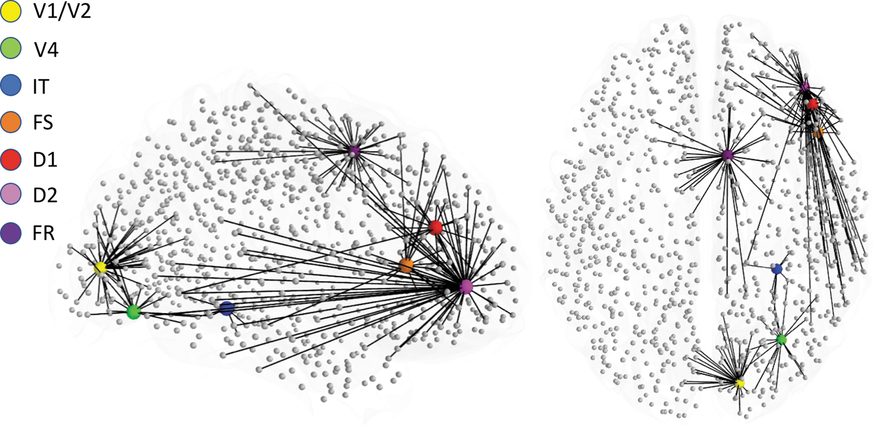
Graphical representation of the location where each of the visual short-term memory nodes was embedded within Hagmann's connectome (Hagmann et al., 2008). Also shown are direct anatomical connections to connectome nodes from each one of the embedded LSNM nodes. LSNM, large-scale neural model.
As already mentioned, we added a structural connectome to provide neural noise to the simulated neural activity during the DMS task, and in return, to receive inputs back from the DMS task nodes. We have described our framework in a previous article (Ulloa and Horwitz, 2016), where we focused on the fMRI BOLD signal generation during the DMS task. In this study, we sought to analyze the FC configurations in brain regions not driving task execution. These “nontask” brain regions exhibit intrinsic activity and because of their reciprocal connections with task-specific brain regions, their neural activity can potentially be modulated during task execution.
We generated 10 virtual subjects by randomly varying the connection weights among brain regions in the structural visual model (see Materials and Methods section for details). We created three experimental conditions: PF, during which simulated subjects with a low “task signal” (roughly equivalent to subjects' attention level during task execution, but see Materials and Methods section for definition of this parameter) are fixating on a small dot; PV, during which subjects passively look at visual shapes; and a DMS task, during which subjects compared two shapes presented within 1.5 sec of each other and responded whether the second shape matched the memory of the first. Each simulated subject performed one 198-sec experiment that consisted of three trial blocks interspersed with rest blocks (see Materials and Methods section for details).
Changes in simulated BOLD activity of nontask brain regions due to different task conditions
Figure 3 shows typical (averaged across neuronal populations within each brain region) neuronal activity for each condition for task-related brain regions during one trial. Figure 3 shows the task regions increasing activity due to both stimuli presentation (V1, V4, IT, FS), short-term memory maintenance (D1, D2), and response (FR). This increase occurs in the PV and DMS conditions (green and red lines) but not in the PF condition (blue line). Thus, the stimulus used in the PF condition (a small dot) does not generate visible changes in the neuronal activity of task regions. The details of the task-related responses shown in Figure 3 have been discussed in detail in previous articles (Horwitz et al., 2005; Ulloa and Horwitz, 2016).
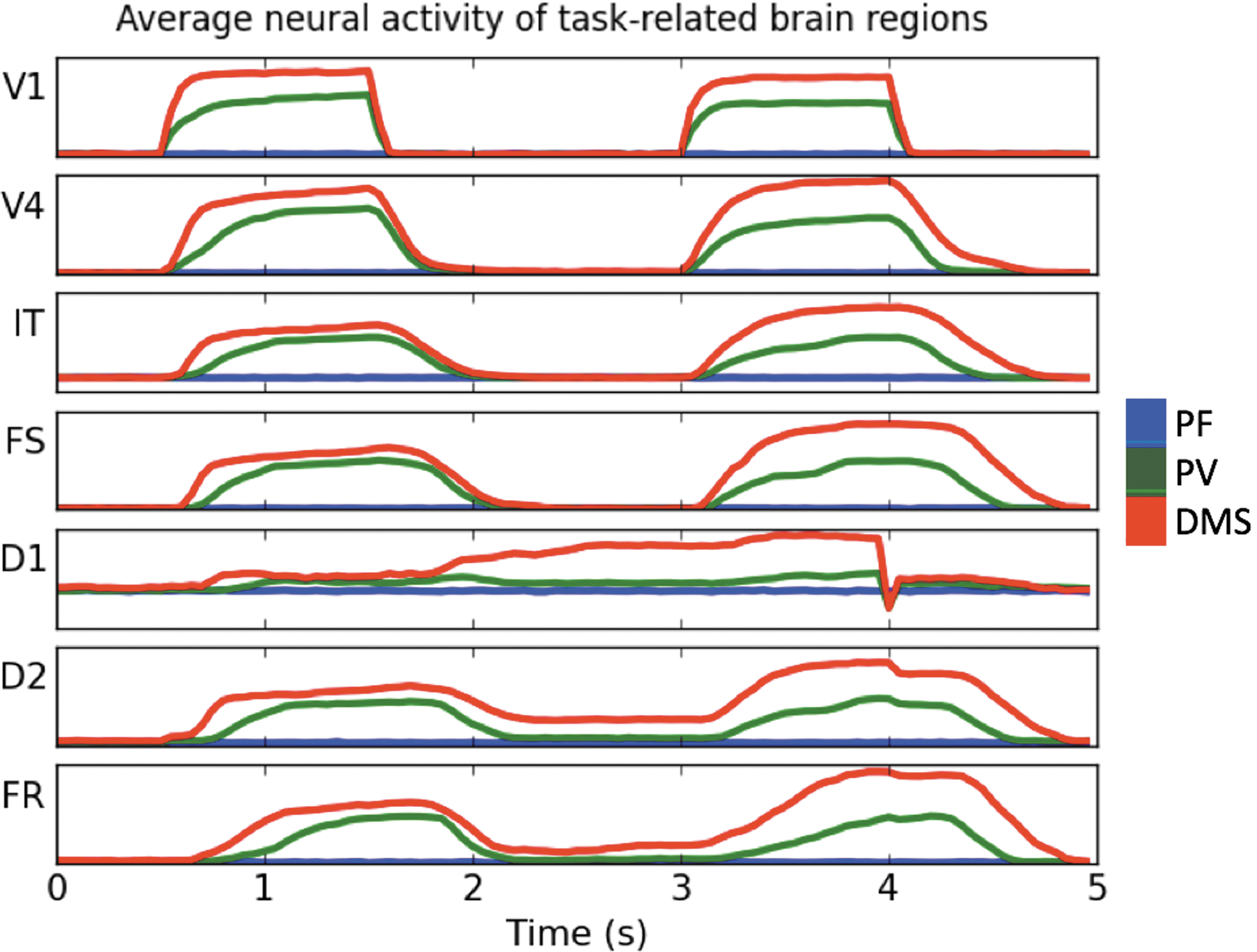
Typical electrical activity in neuronal populations of task-related brain regions during one trial of each of the simulated conditions. PF (blue line), PV (green line), DMS (red line). What is shown is the average across all cortical columns in a brain region. Note that there is a greater electrical activity in the DMS condition than in the PV condition and greater electrical activity in the PV condition than in the PF condition in all model brain regions. DMS, delayed match-to-sample; PF, passive fixation; PV, passive viewing.
Figure 4 shows the BOLD signal averaged across those brain regions with direct anatomical connections to task regions. Figure 2 shows a graphical depiction of the nontask nodes that are directly connected to task nodes. Notice how BOLD activity increases during the task blocks (shaded areas) and how they do so more prominently during DMS than during PV and during PV than during PF. Also notice how that BOLD activity change is larger for some of the brain regions with direct connections to IT, FS, D1, D2, and FR than those regions with direct connections to V1 and V4. This is due to variations in the strength of the connecting weights from task-related nodes to nontask nodes. As shown in Figure 4, changes in all task-related brain regions correlate with BOLD signal changes in nontask brain regions directly connected to them.
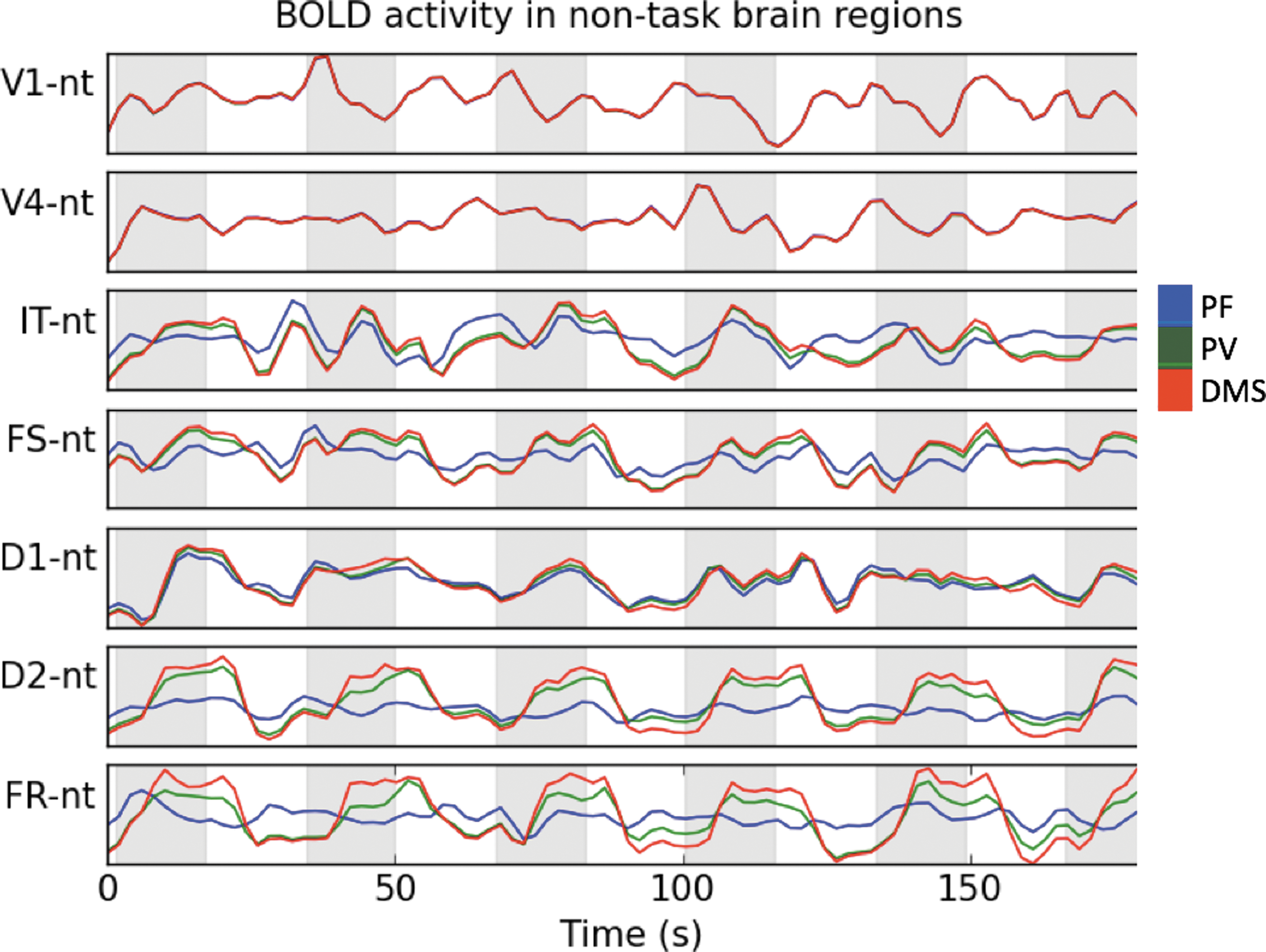
Average BOLD signal of nontask brain regions with direct connections to task-related brain regions. A complete simulated fMRI experiment is shown. Shaded areas correspond to a block of three simulated visual trials for DMS and PV conditions. The nonshaded areas correspond to rest blocks in the PV and DMS conditions. Note that the PF condition consists in passively fixating on a small dot throughout the whole simulation and no rest blocks (see Materials and Methods section for details). BOLD activity increases during the task blocks (shaded areas) and they do so more prominently during DMS than during PV and more prominently during PV than during PF. Also, BOLD activity change is larger for some of the brain regions with direct connections to IT, FS, D1, D2, and FR than those regions with direct connections to V1 and V4. This is due to variations in the strength of the connecting weights from task-related nodes to nontask nodes. BOLD, blood oxygen level-dependent; fMRI, functional magnetic resonance imaging.
Intrinsic FC differences between PF, PV, and DMS conditions
We computed FC matrices for the three simulated conditions and for all subjects. Figure 5 shows the following differences between across-subject averages of FC matrices: PV–PF and DMS–PF. Figure 6 shows scatter plots between PF and PV and between PF and DMS conditions. As shown in Figure 6, the correlation coefficients between PF and both PV and DMS were high (0.90 and 0.83, respectively), demonstrating only small differences in the pair-wise consistency of functional connections across conditions. As already noted, these correlation matrices consist of only connectome nodes (e.g., no LSNM task-based nodes were used to construct these matrices). In summary, there were small changes in the pair-wise FC between PF and PV and between PF and DMS conditions. We next show that differences between conditions become sharper using graph theoretical metrics.
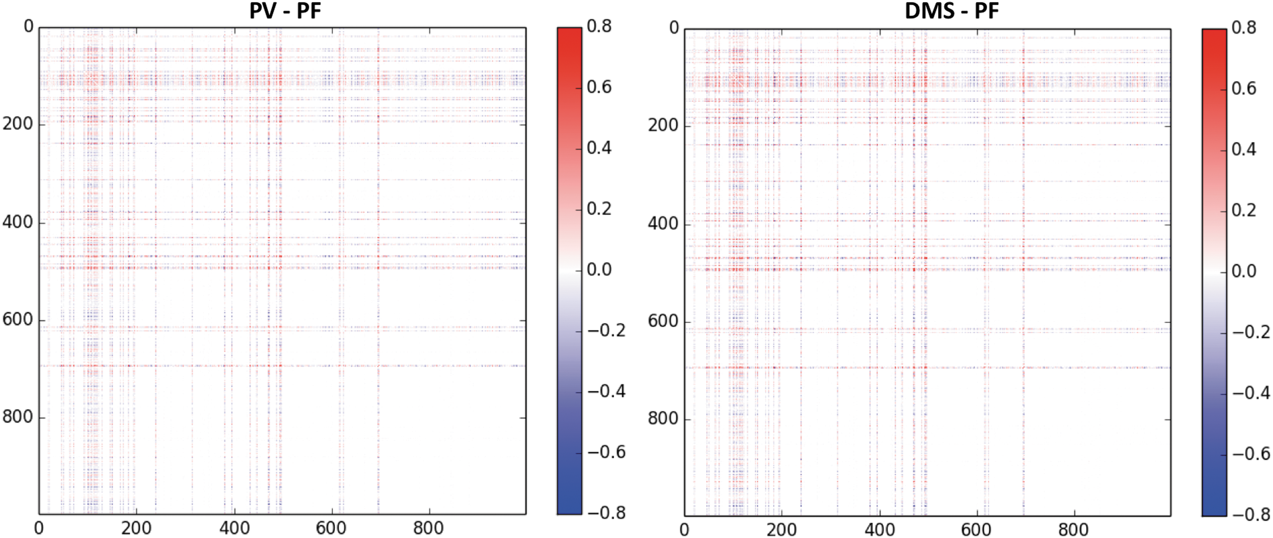
Typical differences (PV–PF) and (DMS–PF) between across-subject averages of the FC matrices obtained from our simulated experiments. Notice that there is an increase in the FC of several pair-wise connections from PF to PV and from PF to DMS. FC, functional connectivity.

Correlation between PF and PV and between PF and DMS weighted FC matrices. The correlation coefficients between PF and both PV and DMS were high (0.90 and 0.83, respectively), demonstrating only small differences in the pair-wise consistency of functional connections across conditions.
Graph theoretical metrics of PF, PV, and DMS conditions
Using graph theoretical methods (Rubinov and Sporns, 2010), we computed network metrics on each of the conditions of our simulation results. Graph theoretical metrics provide ways to quantify both global network organization and local network properties (Bolt et al., 2017; Rubinov and Sporns, 2010). Furthermore, to allow our results to be directly comparable with previous empirical and computational studies (Di et al., 2013; Lee et al., 2017), we selected a subset of eight network metrics (see Materials and Methods section for definition of each metric): global and local efficiencies, average clustering coefficient, characteristic path length, eigenvector centrality, betweenness centrality, participation coefficient, and modularity.
We calculated these metrics using weighted FC matrices for a range of plausible threshold densities (Di et al., 2013). Figure 7 shows across-subject averages of those metrics for a range of network densities (Di et al., 2013). Figure 7 shows that as the task changed from PF to PV to DMS, there was an increase in global efficiency, local efficiency, average clustering coefficient, and average betweenness centrality (mostly at the lowest threshold studied, 5%), and modularity. Conversely, as the task changed from PF to PV to DMS, there was a decrease in average characteristic path length, average eigenvector centrality, and average participation coefficient. Thus, of the eight graph theoretic measures we examined, seven demonstrated clear intrinsic activity differences between the three conditions in the nontask-related nodes.
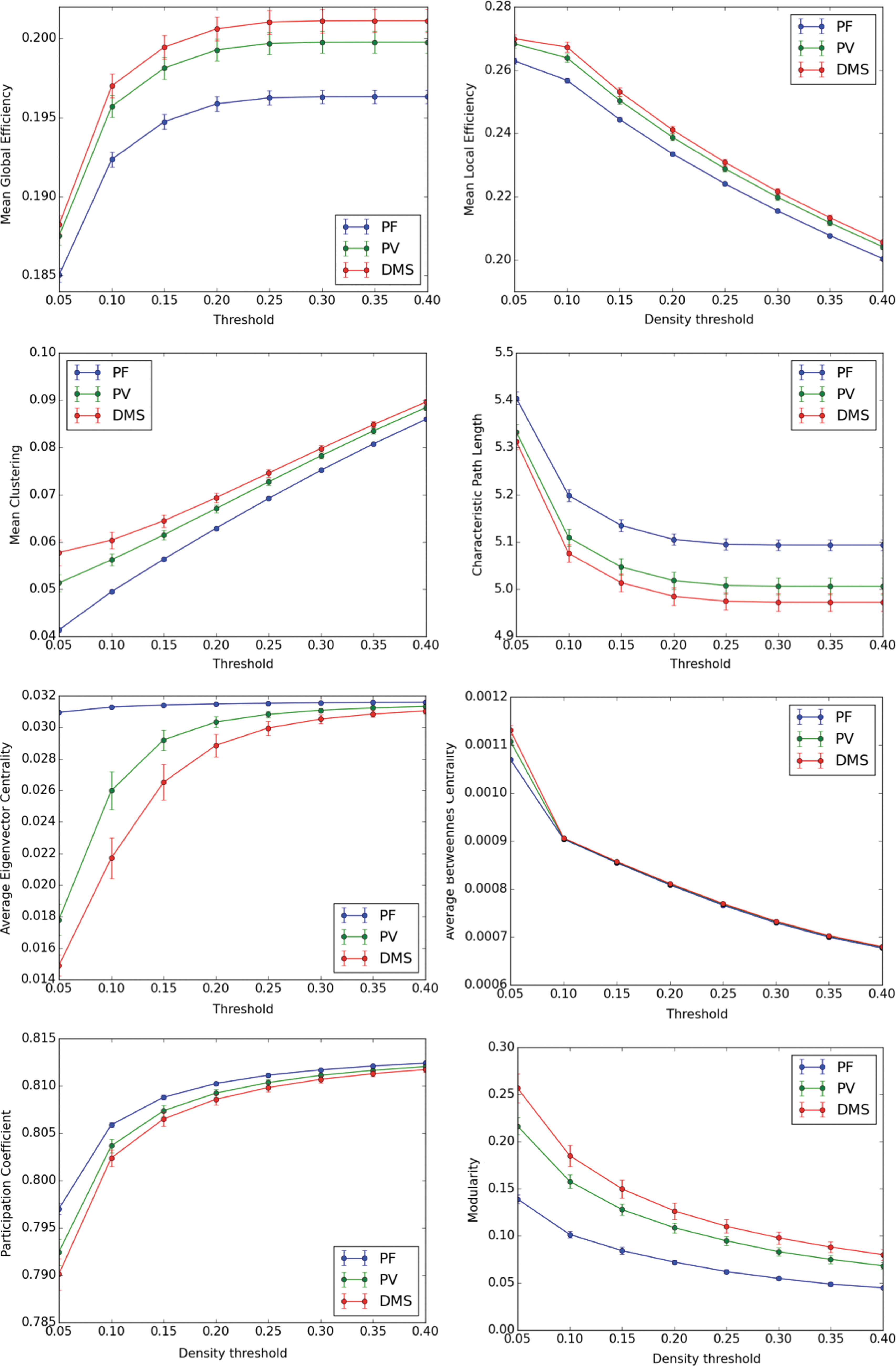
Mean graph theoretical metrics for each condition for a range of network densities (5–40%). Error bars correspond to standard deviation. As the task changed from PF to PV to DMS, there was an increase in global efficiency, local efficiency, average clustering coefficient, average betweenness centrality (mostly at the lowest threshold studied, 5%), and modularity. Conversely, as the task changed from PF to PV to DMS, there was a decrease in average characteristic path length, average eigenvector centrality, and average participation coefficient.
Differences in graph metrics between PF and PV and between PF and DMS
For each graph metric obtained, we computed the relative difference (see Materials and Methods section for details) between PF and PV and between PF and DMS (Fig. 8). We observed significant differences between PF and PV and between PF and DMS in modularity (54.2% ± 8% and 81.3% ± 11.6%, respectively), eigenvector centrality (16.3% ± 1.7% and 22.1% ± 1.8%, respectively) and clustering coefficient (7.9% ± 1.3% and 12.7% ± 2%); smaller changes in global efficiency (1.7% ± 0.2% and 2.4% ± 0.3%), local efficiency (2.2% ± 0.3% and 3.2% ± 0.4%), characteristic path length (1.7% ± 0.1% and 2.3% ± 0.3%), betweenness centrality (1.6% ± 0.3% and 2.6% ± 0.4%), and participation coefficient (0.2% ± 0.1% and 0.4% ± 0.1%). These results indicate that the intrinsic activity metrics that are most changed in the nontask part of the brain, at least for the tasks we simulated, were modularity, eigenvector centrality, and clustering coefficient.
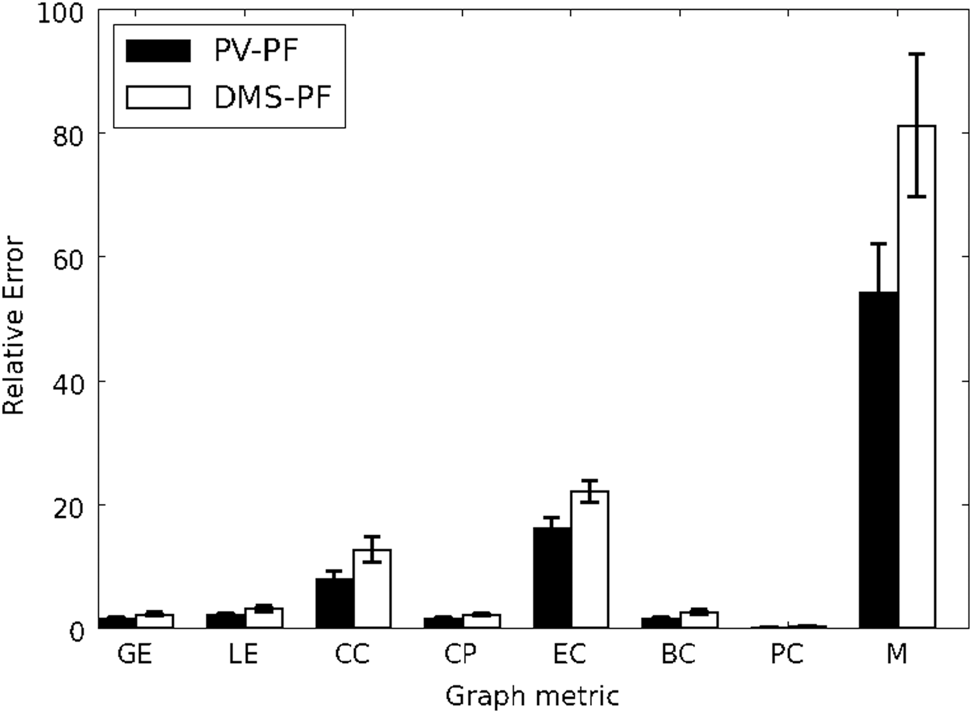
Relative difference between PF and PV and between PF and DMS for each one of the graph metrics shown in Figure 7. Error bars correspond to standard deviation. Although there were significant differences, the major differences were for CC, EC, and M. BC, betweenness centrality; CC, clustering coefficient; CP, characteristic path length; EC, eigenvector centrality; GE, global efficiency; LE, local efficiency; M, modularity; PC, participation coefficient.
Discussion
Using a large-scale computational model of visual short-term memory embedded into an anatomical connectome, we compared simulated intrinsic brain activity of nontask-related brain regions during three tasks: PF, during which simulated subjects with a low “task signal” or “attention” level are fixating on visual stimuli (a small dot); PV, during which subjects passively watch changing visual shapes but take no action; and a DMS task, during which subjects compared two shapes presented within 1.5 sec of each other and responded whether the second shape matched the memory of the first.
The PF condition may be considered equivalent to an RS condition as a PF task has been often used in RS fMRI studies. The key difference between the PF and the PV conditions was that the stimulus during the PF condition was an unchanging small dot, whereas in the PV condition several different and larger stimuli were presented. The key difference between the PV and the DMS conditions was the level of the “task” or attention signal, which was set to a low level in the PV condition and to a high level during the DMS condition.
As discussed in the Materials and Methods section, the task signal level determines whether an input stimulus is going to be retained in short-term memory (Horwitz et al., 2005). In addition, because of feedback connections from D1 in PFC to IT and V4 (see model diagram in Fig. 1), the task signal level indirectly influences neuronal activity in V1, V4, and IT (compare neuronal activity in V1, V4, and IT during different conditions in Fig. 3).
To quantify differences between PF, PV, and DMS conditions, we used pair-wise temporal Pearson correlations (FC matrices) and graph theory metrics of fMRI FC matrices. As already mentioned, both pairwise correlations and graph theoretical metrics have been applied in both task and rest neuroimaging studies to glean information regarding the involvement of mechanisms responsible for brain function.
Although we found small differences between the FC matrices of the simulated conditions, these differences were not particularly impressive. However, we found clear-cut differences in each of the graph theory metrics: graded increases from PF to PV to DMS in global efficiency, local efficiency, clustering coefficient, betweenness centrality, and modularity; and graded decreases from PF to PV to DMS in characteristic path length, eigenvector centrality, and average participation coefficient. Our simulated graph theory results largely agree with empirical studies, as discussed hereunder in detail.
In our computer simulations, the intrinsic brain activity across different conditions is modulated by ongoing neural activity in brain regions engaged in each task (task brain regions). This modulation happens through the strength of the anatomical connections of those brain regions to the rest of the brain (nontask brain regions, see Fig. 2).
When the brain engages in a behavioral task, the activity in neuronal populations driving the task has the potential of reverberating throughout the brain, thereby altering the intrinsic neural activity of neuronal populations not involved in the task. A crucial question is whether one can quantify those changes in intrinsic FC. Computational modeling can be useful in this regard, as it allows us to isolate nontask from task neuronal populations and to convert simulated synaptic activity into neuroimaging time series, which, in turn, can be converted to FC matrices. Furthermore, unlike empirical data, in a computational model we know which neuronal populations participate in the task and which neuronal populations do not.
A commonly used method to simulate the RS is by modeling local neuronal populations with oscillators and using the structural connections obtained from diffusion tractography as connection weights between the model neuronal populations. A parameter search is then conducted to find a global coupling parameter and a white matter conduction speed producing a simulated FC matrix that best matches an empirical FC matrix (Cabral et al., 2011; Ghosh et al., 2008; Gilson, et al., 2016; Hansen et al., 2015; Honey et al., 2009; Lee et al., 2017; Roy et al., 2014; Sanz-Leon et al., 2015). This is the method we used to generate intrinsic activity in the “rest of the brain” of our simulations.
Consistency of pair-wise FC across task conditions
There were small differences between FC matrices PV and PF and between DMS and PF (Fig. 5). There was also a high correlation between the pairs in the FC connectivity matrices between PF and PV and between PF and DMS (Fig. 6). Several researchers have used pair-wise spatial correlations between FC matrices to compare intrinsic with task-evoked conditions (Bolt et al., 2017; Buckner et al., 2009; Cohen and D'Esposito, 2016; Cole et al., 2014; Di et al., 2013; Krienen et al., 2014; Smith et al., 2009).
In general, there is a relatively high spatial correlation (i.e., 0.64–0.9) between a passive condition (such as visual fixation or eyes closed, which are often used to study intrinsic brain activity) and a task condition. Despite such high correlations, differences do exist between passive and task FC, and those differences may be attributable to functional modifications that allow the brain to focus on performing a given task (DeSalvo et al., 2014; Di et al., 2013; Tomasi et al., 2014).
Bolt and colleagues (2017) recently showed that one can have largely consistent FC between passive and task conditions, and at the same time have largely different whole-brain graph theoretical metrics between passive and task conditions. However, a description of the mechanisms behind those seemingly divergent results has not yet been provided.
Increases in global efficiency
Our study resulted in higher global efficiency for DMS than for PV and higher global efficiency for PV than for PF. During the simulated PF condition, the stimulus used is small and mostly activates V1/V2 and V4 and IT areas to a small degree (blue lines in Fig. 3). During the PV condition, the larger stimuli used causes an increase of neuronal activity in V1/V2, V4, IT, FS, D1, D2, and FR (as shown in the trial time series of Fig. 3, green lines), thereby contributing to an increase in neuronal activity of nontask nodes directly connected to task nodes (see green lines in the shaded areas of the time series in Fig. 4).
During the DMS condition, the neuronal activity across the task brain regions is higher than during the PV condition (red lines in Fig. 3). This increase in neuronal activity of task brain regions contributes to an increase in neuronal activity of several of the nontask brain regions with direct connections to task regions during PV and DMS conditions as compared with PF condition (Fig. 4). As shown in the FC differences in Figure 5, there is an increase in the FC of several pair-wise connections from PF to PV and from PF to DMS. This increase in FC contributed to a consistent increase in global efficiency from PF to PV to DMS (Fig. 7).
Graph theoretical measures in empirical studies have consistently shown higher global efficiency during task than during passive conditions [although this could depend on the complexity of the task, but see Cohen and D'Esposito (2016)]. The global efficiency has been found to be higher during a task than during PF (Bolt et al., 2017; Cohen and D'Esposito, 2016), higher during a task than during an eyes closed condition (Fuertinger et al., 2015), greater during a one-back visual memory task than during PV and an eyes closed condition (Wen et al., 2015), and higher for coactivation studies than during RS (Di et al., 2013). In our simulations, the global efficiency is higher during DMS than during PV and PF. This is due to the short-memory task causing an increase of neural activity in brain regions that are, in turn, connected to a widely distributed network in the rest of the brain.
Increases in local efficiency
Our simulations showed a greater local efficiency for DMS than for PV and a greater local efficiency for DMS than for PF. This is consistent with empirical studies showing an increase in local efficiency with increasing task demands (Wen et al., 2015).
Increases in clustering coefficient
Our simulations showed a greater clustering coefficient during DMS than during PV and a greater clustering coefficient during PV than during PF. Previous empirical studies have found a clustering coefficient that is greater for task than during PF (Bolt et al., 2017), lower during a blend of activation studies than during RS (Di et al., 2013), and greater during a language task than during eyes closed (Fuertinger et al., 2015).
Increases in characteristic path length
Our simulations showed smaller characteristic path length during DMS than during PV and smaller characteristic path length during PV than during PF. This is to be expected because as the global efficiency increases, the characteristic path length decreases.
Decreases in mean eigenvector centrality
Our simulations showed smaller eigenvector centrality during DMS than during PV and smaller eigenvector centrality during PV than during PF. The eigenvector centrality metric provides a measure of how well connected a given node is, considering how well connected that node's neighbors are. Thus, eigenvector centrality is recursive because a given node's eigenvector centrality depends on the node's neighbors' eigenvector centrality.
To get a more detailed view of the reason behind smaller mean eigenvector centrality for more complex tasks (Fig. 7), we rendered the eigenvector centrality for each node on axial and sagittal views of the brain (Fig. 9A). Figure 9A shows that as the task complexity increases (from PF to PV to DMS), the eigenvector centrality increases in a few nodes and decreases in most other nodes.
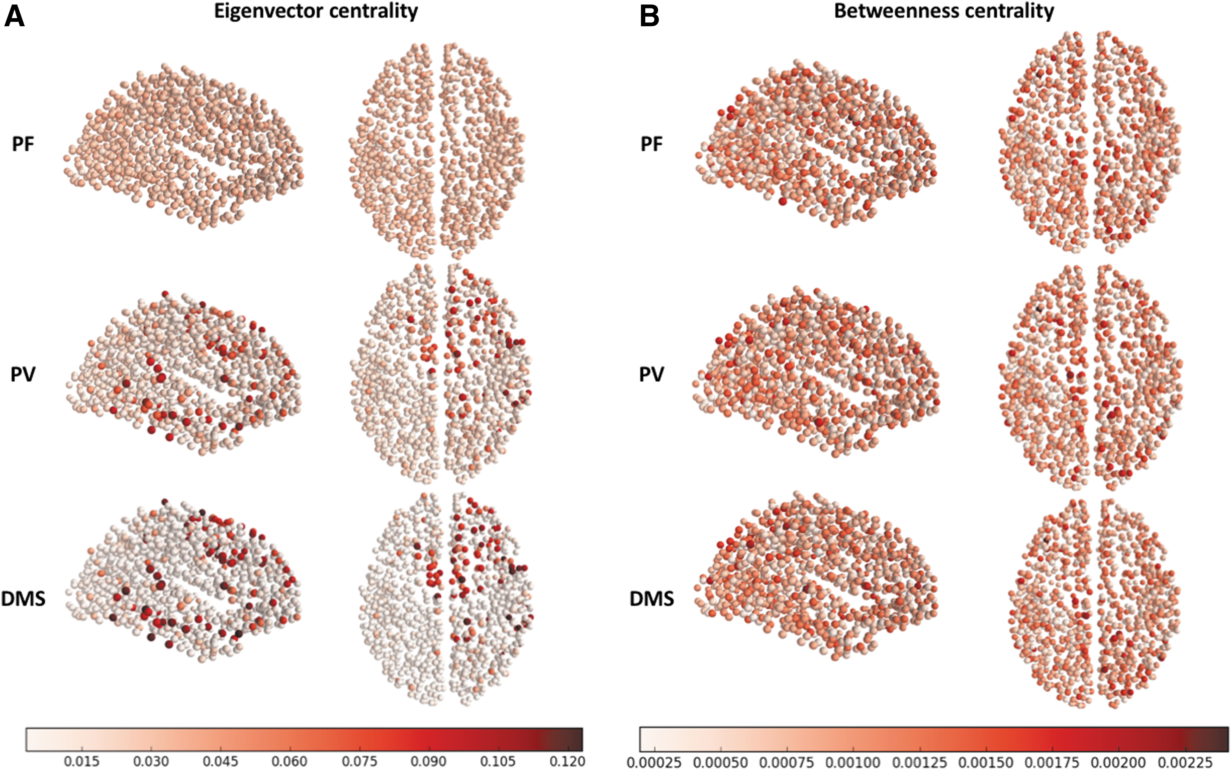
Eigenvector centrality
Thus, on average the eigenvector centrality decreases but the nodal eigenvector centrality in a few nodes increases as the task complexity increases. Note that several of the nodes in which the eigenvector centrality increases during PF and DMS are the nodes that are directly connected to task nodes (compare Fig. 2). The reason the increases are concentrated on the right side of the brain is due to the task nodes, which are embedded in the right side of the brain, having direct connections mostly to the right side of the brain (Fig. 2). Compare the changes in eigenvector centrality with the changes in betweenness centrality (Fig. 7), which remain almost the same during PF, PV, and DMS (Fig. 9B).
Increases in betweenness centrality
Our simulations show a higher betweenness centrality at the lower density threshold (5%), but the average betweenness centrality is very similar across all the other density thresholds (Fig. 7). As already mentioned, the betweenness centrality at each individual node (Fig. 9B) remains relatively constant across conditions. Previous empirical studies have shown a difference in nodal centrality when RS and task are compared (Di et al., 2013).
Decreases in participation coefficient
Our simulations showed greater participation coefficient (in a predefined set of modules) for PF than for PV and greater participation coefficient for PV than for DMS (Fig. 7). Participation coefficient measures each node participation in a set of predefined modules. We used the modules defined by Hagmann and colleagues (2008). Previous studies have shown a higher participation coefficient (between-module connectivity) during PF than during a semantic task (DeSalvo et al., 2014).
Increases in modularity
Our simulations showed a smaller modularity for PF than for PV and smaller modularity for PF than for DMS. Some empirical studies have found a greater modularity metric during RS than during a blend of activation studies (Di et al., 2013), and a greater modularity during PF than during an n-back task using visually presented phonemes (Cohen and D'Esposito, 2016). However, Cohen and D'Esposito (2016) found a similar modularity during PF and a finger tapping task.
Other empirical studies have found that the modularity varies as a function of performance, but here the evidence is also inconsistent. For example, Stevens and colleagues (2012) found a positive correlation between RS modularity and visual working memory capacity and Meunier and colleagues (2014) found a negative correlation between modularity and memory scores in an odor recognition task. In addition, Yue and colleagues (2017) have found significant individual variability in modularity during RS.
Related computational studies comparing RS and task-based FC.
Two previous computational approaches have compared the intrinsic brain activity obtained during RS versus that obtained during task; however, none of those models was specifically concerned with quantifying intrinsic activity differences between different task conditions (which is the goal of our article). The first of those studies, by Ponce-Alvarez and colleagues (2015), simulated RS using a set of mean field equations (excitatory–inhibitory pairs) interconnected by the anatomical connections of a 66-node connectome. A visual task was approximated by applying external stimulation (stationary inputs) to visual nodes during the RS simulation. Ponce-Alvarez's model revealed a decreased synaptic activity variability during the visual task as compared with the RS condition.
The second computational study comparing task versus rest (Cole et al., 2016) similarly applied stationary inputs to a set of neighboring nodes in a simplified computational model to simulate six different tasks. Cole and colleagues used the FC strengths during a passive task to predict the fMRI task activation of a held-out brain region. They did this for every one of the simulated brain areas so as to produce a prediction of the fMRI activity in each of the simulated brain areas.
Caveats and limitations of our study
Different passive experimental conditions have been used in neuroimaging to study intrinsic brain activity [also referred to as the “RS”] (Biswal et al., 1995; Fox et al., 2006; Greicius et al., 2003). Three of the conditions most commonly used as a RS condition are PF, eyes open with no fixation, and eyes closed. Yan and colleagues (2009) found significantly higher FC in DMN brain areas during eyes open than during eyes closed condition.
It is also important to emphasize that the fMRI results can vary depending on several other factors, including how a RS task is defined (Van Dijk et al., 2010; Yan et al., 2009), which task instructions are given to subjects (Benjamin et al., 2010), and whether subjects were engaged in a task before RS (Waites et al., 2005). Thus, although one can compare (within the limitations outlined hereunder) the results of our study with empirical studies using PF, our results cannot be directly extrapolated to all RS-fMRI studies.
One way in which the simulations presented here are different from our previous article (Ulloa and Horwitz, 2016) is that the model response units have been relocated from PFC to PreSMA.
The relocation of the response units to PreSMA is based on an fMRI study by Pessoa and colleagues (2002), who found an increase in BOLD fMRI in the PreSMA area at the end of the delay period during a visual working memory task. In addition, a study by Petit and colleagues (1998) has also demonstrated BOLD fMRI activity in the PreSMA area during a working memory task. The relocation from previous studies from our laboratory of the model response units to PreSMA makes biological sense as it better reflects the complexity of the task we are trying to simulate. The identification of realistic locations within the brain for each one of the model units is crucial as different locations of task-related modules will modulate different nontask nodes in the connectome, thereby producing different FC configurations.
One of the limitations of our study is that our model connectome does not have other sensory systems apart from the visual system. Therefore, one should exercise caution when comparing FC matrices of our simulation with empirical matrices as the empirical matrices would contain higher FC that are the result of other sensory systems being activated by either intrinsic or extrinsic processes. For example, in an fMRI scanner room, there is significant auditory stimulation (scanner noise) as well as somatosensory input, which we have not simulated in this study.
In our simulations, we only embedded the visual model in the right hemisphere. As a result, the intrinsic activity was mostly localized to the right hemisphere. Nonetheless, there were significant intrinsic activity changes in the left hemisphere, and those were caused by structural connectivity between both hemispheres.
Another limitation of our study is that the weights of the structural connectome used in this article are undirected and we assumed all connection weights to be excitatory. It is well known that diffusion tractography has serious limitations as it produces a significant number of false positives (Maier-Hein et al., 2017), has relatively low resolution, and measures white tracts only indirectly (Jbabdi et al., 2015). Some researchers have simulated whole brain activity using connectome data sets obtained from reconstructions of retrograde tracer injections in macaques (Chaudhuri et al., 2015) or a composite of diffusion spectrum imaging in humans and macaque tracer data (Sanz-Leon et al., 2015).
Despite the low resolution and lack of sign and direction of the human tractography data, we decided to use it as it allowed the “brain regions” of our task-based simulator to be embedded into plausible locations within the structural connectome.
Conclusions
In conclusion, we used our large-scale neural modeling framework to quantitatively compare neural dynamics of nontask brain regions during PF, PV, and a visual short-term memory task. We were able to obtain quantitative measures of differences in simulated FC by using graph theoretical methods. Our simulated graph theory results largely agreed with experiments. We were also able to relate those network-level changes to the underlying model mechanisms. We showed that we can use computational modeling, FC, and graph theoretical metrics to quantify changes in intrinsic FC of nontask brain regions due to increasing task demands.
Our study is relevant to the characterization of intrinsic brain activity differences between passive and active task conditions and to the use of neural modeling in the design of empirical studies and the comparison of competing hypothesis of brain function.
Footnotes
Acknowledgments
This research was funded by the Division of Intramural Research of the National Institute on Deafness and Other Communication Disorders. This study utilized the computational resources of the NIH HPC Biowulf cluster (
Author Disclosure Statement
A.U. is the founder and owner of Neural Bytes LLC, a for-profit company.
References
Supplementary Material
Please find the following supplemental material available below.
For Open Access articles published under a Creative Commons License, all supplemental material carries the same license as the article it is associated with.
For non-Open Access articles published, all supplemental material carries a non-exclusive license, and permission requests for re-use of supplemental material or any part of supplemental material shall be sent directly to the copyright owner as specified in the copyright notice associated with the article.